Google matrix of business process management

Abstract

Development of efficient business process models and determination of their characteristic properties are subject of intense interdisciplinary research. Here, we consider a business process model as a directed graph. Its nodes correspond to the units identified by the modeler and the link direction indicates the causal dependencies between units. It is of primary interest to obtain the stationary flow on such a directed graph, which corresponds to the steady-state of a firm during the business process. Following the ideas developed recently for the World Wide Web, we construct the Google matrix for our business process model and analyze its spectral properties. The importance of nodes is characterized by PageRank and recently proposed CheiRank and 2DRank, respectively. The results show that this two-dimensional ranking gives a significant information about the influence and communication properties of business model units. We argue that the Google matrix method, described here, provides a new efficient tool helping companies to make their decisions on how to evolve in the exceedingly dynamic global market.

1 Introduction

Business process models are dynamical systems that describe the interdependencies of functional units, or components, on a micro- or macroeconomic level. They depict the way a company works and eventually makes money with the strategy it uses. The efficiency of a model is primarily determined by the help a model can give for strategic decisions, e.g. if a reorientation of products or marketing is needed due to changes in the market or opportunities because of technological developments (see e.g. Sterman-01 ; bpm and Refs. therein).

The building of a business model is a complicated task, because all important units in the company value production must be identified and properly linked at a certain level of modeling. This involves a cancellation of non-important unit, which might be even harder. What modelers do further is a qualitative identification if a unit positively or negatively stimulates a linked one (amplification or damping, respectively). This yields a directed graph, where the units of the model are linked and the direction reflects causality. The next step towards quantitative modeling is the prescription of a functional dependence of the units, which is basically a very heuristic procedure. Clearly, the functions have to be nonlinear, because a growth to plus/minus infinity is not allowed, so typical functions are of sigmoid-type, on the other hand minimal models are of predator-prey type, well known from biology. This reflects the modern point of view of a company as a quasi-organic, dynamical system.

In this work we introduce and analyze the Google Business Process Model (GBPM) of a real consulting company Grasl-08 whose major product is of intellectual nature. The detailed description of the original dynamical model can be found in Grasl-08 and thus we do not present it here. The model describes a dynamical workflow propagation (see e.g. leymann1 ; leymann2 ) which is simulated by certain dynamical equations.

In our approach we trace parallels and similarities between the directed graph of this model and the Google matrix approach used for the ranking of the World Wide Web (WWW) brin ; meyer ; avrach3 . Thus, we investigate only the model graph and do not enter the subject of dynamical simulations, because we want to reveal the underlying structure of the stationary state of the model without using the quite heuristic functional dependencies which need to be further supported by statistical analysis and measurement. This is not to say that the latter is a wrong approach, however the determination of the stationary density by the application of the PageRank algorithm for the Google matrix, which is a variant of Frobenius–Perron operator meyer , is a very powerful and well–established technique which gives fundamental results on the network without solving the dynamical equations and using a vast study of parameter variations.

Indeed, the construction of the Google matrix for the WWW and the determination of the stationary probability distribution over WWW network via the PageRank algorithm has been proposed by Brin and Page brin and by now it became a powerful tool for classification of the WWW nodes (see e.g. meyer ; avrach3 ; donato ; upfal ). The approach based on the Google matrix construction for a directed network is rather general and finds applications for various types of networks including university WWW networks giraud , Ulam networks of dynamical maps zhirov2010ul ; ermann2010ul , brain neural networks brain , procedure call network of Linux kernel aliklinux ; leolinux , hyperlink network of Wikipedia articles zhirovwiki . PageRank finds also applications in blog analysis fortunato1 , citation network of Phys. Rev. redner ; fortunato2 , and food flow network between species in ecosystems food .

In this work we extend this approach to the network of business management. How is the model built? Basically, one has identified major components of the company, which are refined in their dynamics in respective subcomponents. By construction, the model is hierarchical, but links between components can be set according to the needs of the modeler. We only mention here the components and the nodes in the top component: managers, consultants,…; subcomponents are: top, consultants, products, proposals, customers, …. . The full list of nodes and links between them are given in Appendix. Depending on the business process, one of the nodes is the most important one, followed by others. This is the value of our method: we identify without any bias the most important components in a model. This provides an extremely helpful information. If these components are not the ones wished by the shareholders or management, respectively, the model has to be changed and adapted. Since the computation is not very costly this gives a tool to simulate small changes, e.g. by linking different nodes, and studying their effect on the business process model. We consider the GBPM as a first step in the application of the Google matrix analysis to the business process management. Next steps should extend this approach and take into account actual workflow between nodes inside a companyleymann1 ; leymann2 .

Our network is small in comparison of typical applications of Google Matrix, like the WWW donato ; upfal , Linux kernel network aliklinux ; leolinux or Wikipedia network zhirovwiki . It consists of 175 nodes only and is graphically displayed in Fig. 1. This size is comparable with the one of food network in ecosystems food . Our purpose is an elementary study of the network properties using the spectral characteristics of the Google matrix, PageRank and recently introduced CheiRank and 2DRank such that the order $10^{2}$ is sufficient; the latter ranking algorithms are explained in detail below, Most big business models are proprietary (for understandable reasons), and an application of the Google matrix method is straightforward.

Figure 1: Google Business Process Model with links taken from Grasl-08 . The network is structured into several subgraphs reflecting the functionality of the model. The names (or meaning) of the nodes and links between them are listed in the Appendix.

Let us have a look on the network in terms of connectivity: the distribution of ingoing and outgoing links is shown in Fig. 2. Of course, with only one decade available it is useless to try to identify exact scaling behaviour; nevertheless the global distribution is compatible with power law scaling $f(d)\sim d^{-\nu}$ at $\nu\approx 3$. The exponent $\nu=3$ is not so far from the exponent $\nu=2.1$ and $2.7$ found for the WWW for ingoing and outgoing link distributions respectively donato ; upfal . It will be interesting to investigate the generic scaling of business models in the future for networks of larger size.

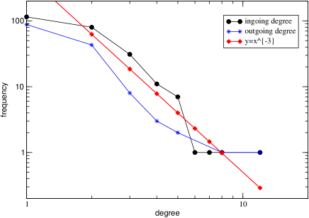
Figure 2: (Color online) Distribution of ingoing (black points) and outgoing (blue points) links. An approximate global power law scaling with the exponent 3 is shown by the straight red line.

2 Method

The Google matrix $G$ underlies the determination of PageRank brin , which is a tool used by virtually every Internet user when issuing an Internet search for some keywords. This approach gives a powerful and general way to analyze networks. For the construction of the Google matrix we use the procedure described in brin ; meyer :

$$G_{ij}=\alpha S_{ij}+(1-\alpha)/N\;,$$ (1)

where $S_{ij}$ is the normalized adjacency matrix of the graph. The elements of the adjacency matrix are zero (if there is no link) or one (if there is a link). Due to the normalization the sum of all elements inside one column is equal to unity. Columns with zeros only are replaced by $(1/N,\dots,1/N)$, with $N$ being the network size. Because it is a full stochastic matrix of a Markov chain, the matrix ${\bf S}$ has N eigenvalues $\lambda_{i}$, $i=1,\dots,N$ which are generally complex. In agreement with the Perron-Frobenius theorem (see e.g. meyer ) the largest eigenvalue is $\lambda_{1}=1$. The damping parameter $\alpha$ denotes the possibility for a random surfer on the graph to jump to any other node. Its effect is to bound away the eigenvalues with absolute value smaller than one: $|\lambda_{i}|\leq\alpha<1$ for $i>1$. A typical value, used as well for the WWW search, is $\alpha=0.85$, however this choice can be varied without essential impact on the results presented below. The right eigenvectors, $\psi_{i}$, are defined by ${\bf G}\psi_{i}=\lambda_{i}\psi_{i}$, cf. meyer ; giraud . The PageRank vector is the one with $\lambda=1$, and since ${\bf G}$ is a Frobenius-Perron operator, the corresponding right eigenvector, $\psi_{1}=(P(1),\dots,P(N))^{T}$ gives the stationary probability density $P(i)$ that a random surfer is found at site $i$ with $\sum_{i}P(i)=1$. Once it is found, the nodes are sorted according to decreasing $P(i)$, the node rank in this index, $K(i)$ corresponds to its relevance.

Other eigenvalues correspond to non-stationary, decaying modes. They are of transient nature and may play an important role in non-stationary considerations, because they may live for a long time before dying out. This is, however, not the focus of this work.

3 CheiRank versus PageRank

In a nutshell, the procedure uses the idea that a node is not only relevant if it is highly linked. One has also to take into account the relevance of the nodes pointing to it. Since this is an iterative procedure, the PageRank vector can be easily computed by the so–called power-iteration using consecutive multiplication of initially random vector on the Google matrix meyer . Of course, this vector is the most important one, because it represents the stationary distribution on the graph. The relaxation process to the steady-state given by the PageRank is affected by the eigenmodes with $|\lambda|$ close to $\alpha$. It is known that for the WWW there are many eigenvalues which are close or even equal to $\alpha$ (see e.g. meyer ; giraud ). The spectrum of the Google matrix ${\bf G}$ of the GBPM is shown in the left panel of Fig. 3. The eigenvalue next after $\lambda=1$ is $\lambda_{2}=0.706$ and other eigenvalues have $|\lambda|<0.52$. There are only about 14% of eigenvalues with $|\lambda|>0.1$ that gives an indication on a possibility of appearance of the fractal Weyl law for such type of networks of larger size $N$ in analogy with the Linux kernel network analyzed in aliklinux ; leolinux . The spectrum of the Google matrix ${\bf G^{*}}$, obtained from the network with the inversed direction of links, is shown in the right panel of Fig. 3, its characteristics are similar to those of matrix ${\bf G}$.

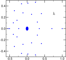
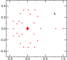
Figure 3: (Color online) Distributions of eigenvalues $\lambda$ of the Google matrix at $\alpha=0.85$ in the complex plane for matrix ${\bf G}$ (left panel) and matrix ${\bf G^{*}}$ with inverted link directions (right panel).

The PageRank probability $P(i)$ for our business model is shown in Fig. 4 (top panel) as a function of rank $K(i)$. Surprisingly, there is no dominant node, which means that this company is quite democratic - in terms of relevance. The first five nodes are: Identified Contact Loss (33), Identified Contacts (32), Projects (5), Consultants (2), Delivery Project Completion (87). The numbers in brackets denote the node indices, cf. the Appendix. Managers (node index 1) do not appear before rank 18. This is quite surprising, since the management is expected to be at least among top ten positions. How can one understand that behaviour? The management plays typically the role of coordinating projects and keeping all together, which means that they decide which points are most important and have many outgoing links related to orders given to others. However, the PageRank is proportional in average to the number of ingoing links meyer . This implies the management units are not most important according to the PageRank since they do not have a large number of ingoing links (not many units give order to managers). In the considered model of a consulting company the most relevant units are the customers, or contacts. Without them, no business is made, especially for consulting. The first two ranks can be explained by this. The following ranks are Projects and Consultants. Of course, without good projects and correspondingly good workers the firm will die, so this is of vital relevance. Rank 5 again involves projects, this time their delivery. This means that in this model the way the projects are completed is given a high importance. This might not be necessarily true in all cases, however for the model of the firm under consideration it is. We recognize that in this view the result makes perfect sense: customers, products and consultants are the most relevant units in the model of a consulting firm. Such a firm can only survive when its consultants are top level and its products are alike - and if there are customers. The management is responsible only to get the firm running well. This result may be surprising, but reveals the power of the method. This means as well that the most attention for refinement of the model should be put on the top nodes given above. Nevertheless, one expects that the management plays somehow a very influential role.

It is interesting to note that a similar situation takes place for the procedure call network of the Linux kernel as it was shown in aliklinux . Indeed, for this network the PageRank gives at the top procedures which are often pointed on but which are not so much important for the code functionality. Thus it was proposed aliklinux to characterize the network also by the PageRank of the Google matrix obtained from the network with inversed link directions. The rank $P^{*}(i)$ of this inversed matrix ${\bf G^{*}}$, named as the CheiRank zhirovwiki , places on first positions rather influential code procedures. Hence, it is natural to use the CheiRank also for our model of business process management.

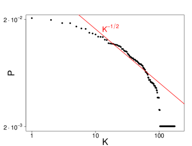
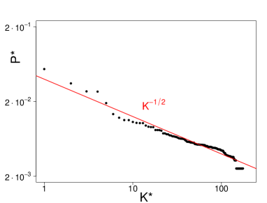
Figure 4: Top panel: probability of PageRank vector $P(i)$ as a function of PagRank $K(i)$ in log-log scale. Bottom panel: probability of CheiRank vector $P^{*}(i)$ in log-log scale. The straight lines show the approximate power law dependence with the slope $1/(\nu-1)=1/2$, corresponding the the average slope $\nu=3$ shown in Fig. 2.

And indeed, using the CheiRank, introduced in aliklinux we obtain an adequate result. It corresponds to the stationary distribution, $P^{*}(i)$, of the inverted flow, or the information returned from the nodes to their precedent ones. Thus, it describes the influence or communication ranking of the nodes. Again, the eigenvector with the eigenvalue 1 is computed and sorted according to the magnitude of the entries. This yields a new rank, $K^{*}(i)$, the mentioned CheiRank. The result of the computation of $P^{*}(i)$ vs. $K^{*}(i)$ is displayed in Fig. 4. (bottom panel). Here, we can also give a tentative scaling $P^{*}(i)\sim K^{1/(\nu-1)}$ which must be compared and verified, respectively, with other business models of larger size. While the distribution of $P(i)\sim K^{1/(\nu-1)}$ is proportional to the distribution of ingoing links, the distribution of $P^{*}(i)$ is proportional to the distribution of outgoing links (see e.g. meyer ; avrach3 ; giraud ; aliklinux ). Due to a small size of our network we do not try to use different values of $\nu$ for ingoing and outgoing links and for $P$ and $P^{*}$ respectively. According to the CheiRank the top nodes are: Principals (1), Projects (5), Consultants (2), Customers (6), Contacts (7). The management now has clearly first position in the ranking which is fully logical, since any management decision influences the whole company, while the management is not necessarily the most important component, as explained above.

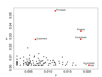
Figure 5: (Color online) Distribution of nodes in the plane of probabilities of PageRank $P(i)$ and CheiRank $P^{*}(i)$. The marked nodes illustrate the first four nodes in Chei rank (Principals, Projects, Consultants, Customers), and the top node in PageRank (Identified Contacts Loss)

Following aliklinux we also use the joint distribution of nodes in the plane of probabilities $(P(i),P^{*}(i))$ of PageRank and CheiRank shown in Fig. 5. That way, we see both ranks at once and can decide which emphasis to put, defining importance in a new way. In this sense, the most important nodes are indicated in Fig. 5. The distribution of all nodes in the plane of PageRank and CheiRank $(K,K^{*})$ is shown in Fig. 6. In the plane $(K,K^{*})$ the most important nodes are those with the smallest values of $K$ and $K^{*}$. The zoom of this region of the plane is shown in Fig. 7.

Of course, nodes might be both relevant (well-known) and influential (communicative). This can be characterized by the correlator $\kappa$ between PageRank and CheiRank which is defined as

$$\kappa=N\sum_{i}P(i)P^{*}(i)-1\;.$$ (2)

For the WWW university networks aliklinux and Wikipedia network zhirovwiki it was found that the correlator is rather large with $\kappa\approx 4$ while for the Linux kernel network one has very small correlator $\kappa\approx-0.05\ll 1$. For the GBPM we have $\kappa=0.164$ showing that there is practically no correlations between nodes with large number of outgoing and ingoing links. Thus the GBPM network has more similarities with the Linux kernel network in contrast to the WWW and Wikipedia networks which are characterized by high correlations between nodes which are highly known (high PageRank) and highly communicative (high CheiRank).

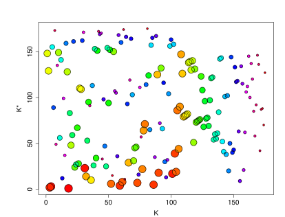
Figure 6: (Color online) Distribution of nodes in the plane of PageRank $K$ and CheiRank $K^{*}$, size of circles and their color is proportional to their listing node index with large radius (red color) for small index and small radius (blue-rosé) for large index.

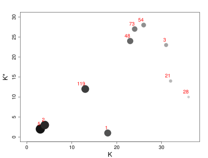
Figure 7: Zoom of the distribution of nodes in the plane of PageRank $K$ and CheiRank $K^{*}$ in the region of small $K,K^{*}$ values. Numbers near circles give the listing node index, grayness is proportional to 2DRank $K_{2}$ with black for minimum and light gray for maximum $K_{2}$ (see Appendix).

With the appearance of CheiRank all nodes are now distributed in a two-dimensional plane (see Figs. 5,6,7). How can one combine both rankings in a way to find nodes which are both very relevant and influential? There are many ways to find such a single-valued one-dimensional ranking which combines $K$ and $K^{*}$: one can think of the distance $(K^{2}+{K^{*}}^{2})$, or the absolute value, or some other combination of $K$ and $K^{*}$. Since $P(K)$ and $P^{*}(K^{*})$ are monotonic functions the plane $(K,K^{*})$ is mapped into $(P,P^{*})$ plane in a unique way.

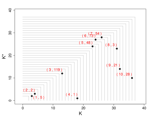
Figure 8: Illustration of the 2DRank algorithm to find rank $K_{2}$ which combines PageRank $K$ and CheiRank $K^{*}$. Specific nodes are drawn in the $(K,K^{*})$ plane when crawling through the squares, indicated by the grey lines, from small to large $(K,K^{*})$ the nodes are labeled by $K_{2}$; numbers in brackets $(K2(i),i)$ give the value of found 2DRank $K_{2}$ and the values of listing node index $i$. One recognizes that at most 2 nodes can be found on a square edge, and some edges might be empty.

A convenient way to order all nodes of the two-dimensional plane on a one-dimensional line was proposed in zhirovwiki for Wikipedia articles being named 2DRank $K_{2}$. This rank is described by the algorithm presented below; it is dubbed 2DRank $K_{2}$, since it combines the two ranks discussed above. Remember that a ranking is basically a list of pairs (rank and nodes index), in our case $K2,i$, or simply $K_{2}(i)$. By $K_{2}$, we also use this ordering of nodes by the following, quite intuitive criterion: we look progressively if a point $(K,K^{*})$ lies on the square $j\times j$, where $j$ is a running index starting at 1. Since the ordering is unique, there are only two possibilities for this to occur: either $K=j$ or $K^{*}=j$. It may happen, that neither $K$ nor $K^{*}$ lies on the square, then one increases $j$ by one and compares again with $(K,K^{*})$. The initial $K_{2}$ list is empty. E.g. if there is no point with $K=1$ and $K^{*}=1$, then the first square $1\times 1$ has no point on it and the next square $2\times 2$ is considered. The algorithm works by setting $j=1$, then we look if $K=j$, if yes, $i(K,K^{*})$ is determined and added to the list $K_{2}(i)$ whose own running index is increased; then we apply this procedure to $K^{*}$: if $K^{*}=j$, the node index $i(K,K^{*})$ is determined and added to the list $K_{2}(i)$. Since there are no more points to check, we step from $j$ to $j+1$. The algorithm is finished if all nodes $i$ have been visited. We can deliberately choose if we first look for $K$ or $K^{*}$ (we have chosen first $K$). The procedure is illustrated for the first ten nodes in K2 ranking in Fig. 8.

According to this 2DRank algorithm we find for the first five nodes in 2DRank $K_{2}$: Projects (5), Consultants (2), Hire Rate (119), Principals (1), Required Delivery Proposal Effort (48). The principals are still not the most relevant node, but obviously this ranking gives a quite balanced characterization of the business process management under consideration.

Top 30 nodes ordered according to PageRank, CheiRank and 2DRank are given in Appendix. Ranking of all nodes is available at the website gbpmpage .

4 Discussion

We have presented a powerful method which quantitatively describes the business process management in terms of the Google matrix, its eigenvectors and eigenvalues. The application of the method yields the stationary distribution on the directed graph which describes the business process of a concrete company in the frame of our GBPM. Our results show that the importance and influence of the units of business process are well characterized by two-dimensional ranking in the plane defined by PageRank and CheiRank. These ranks show that certain units (e.g. Contacts) perform important tasks being highlighted by PageRank, while other units (e.g. Principals ) realize influential communication processes highlighted by CheiRank. Thus the two-dimensional ranking described here establishes a broad and detailed characterization of main operational units of business process management. In contrast to the WWW university networks and Wikipedia network, the network of GBPM has rather small correlation between top units of PageRank and CheiRank that stresses a clear separation between communication and realization tasks of business process. In this respect the GBPM network is more similar to the procedure call network of Linux kernel which also has small correlation between these two ranks.

Of course, the approach developed here is in its initial stage and more advanced business process modeling will need weighted graphs with subgraphs for the flows of work, information, money, products, etc. These generalizations are straightforward and can be constructed at next more advanced stage. A study of changes in the model is quick and straightforward, such that systematic studies of future activities of a company are now feasible without sometimes very heuristic equations which can be used at a final modeling stage. But now one is relieved from the task to determine fine–tune parameters and equations each time a model is changed. We expect these results to have significant impact in econometry for the evaluation of small, middle-size and large-scale models of business process management. The application to macro-economy is straightforward, and global flows might be characterized by the GBPM procedure.

Appendix

List of Nodes

(node number is followed by its name and comma):

1 Principals, 2 Consultants, 3 Value, 4 Products, 5 Projects, 6 Customers, 7 Contacts, 8 Heads Of Branch, 9 Total Principals, 10 Maximum Principal Proposal Effort, 11 Maximum Principal Hiring Effort, 12 Average Principal Work Effort, 13 Maximum Principal Work Effort, 14 Maximum Project Time Share, 15 Maximum Contact Maintenance Effort, 16 Maximum Product Effort, 17 Contact Maintenance Effort, 18 Maximum Contact Maintenace Time Share, 19 Maximum Principal Project Effort, 20 Contacting Effort, 21 Qualified Contacts, 22 Required Contact Maintenance Effort, 23 Qualified Contact Maintenance Effort, 24 Qualified Contact Lifetime, 25 Maximum Qualified Contacts, 26 Minimum Qualification Duration, 27 Qualification Fraction, 28 Contact Qualification Rate, 29 Qualified Contact Loss, 30 Maximum Qualification Rate, 31 Contact Identification, 32 Identified Contacts, 33 Identified Contact Loss, 34 New Customer Contact Potential, 35 Identificaton Duration, 36 Identified Contact Lifetime, 37 Identification Fraction, 38 Delivery Proposal Effort, 39 New Delivery Proposal Effort, 40 Delivery Proposal Writing Effort, 41 Principal Delivery Proposal Effort, 42 Delivery Proposal Effort Share, 43 Delivery Proposal Closing Rate, 44 Delivery Proposal Writing Rate, 45 Minimum Duration Per Delivery Proposal, 46 Delivery Project Effort, 47 Effort Per Delivery Proposal, 48 Required Delivery Proposal Effort, 49 Delivery Lead Success Rate, 50 Delivery Proposal Effort Fraction, 51 First Time Delivery Lead Success, 52 Repeat Delivery Lead Success, 53 Repeat Delivery Lead Fraction, 54 Repeat Delivery Lead Generation, 55 Repeat Delivery Leads, 56 Repeat Delivery Lead Success, 57 Repeat Delivery Proposals, 58 Repeat Delivery Proposal Success, 59 Repeat Delivery Lead Loss, 60 Repeat Delivery Proposal Loss, 61 Delivery Project Effort, 62 Customer Delivery Lead Generation Duration, 63 Delivery Lead Closing Duration, 64 Delivery Proposal Closing Rate, 65 Lead Generation Pressure, 66 Effect Of Delivery Project Per Principal, 67 Repeat Delivery Lead Success Fraction, 68 Repeat Delivery Proposal Success Fraction, 69 First Time Delivery Lead Generation Duration, 70 First Time Delivery Leads, 71 First Time Delivery Proposals, 72 Delivery Projects Won, 73 First Time Delivery Lead Generation, 74 First Time Delivery Lead Success, 75 First Time Delivery Proposal Success, 76 First Time Delivery Lead Fraction, 77 First Time Delivery LeadLoss, 78 First Time Delivery Proposal Loss, 79 Delivery Proposal Closing Rate, 80 Delivery Lead Closing Duration, 81 First Time Delivery Proposal Success Fraction, 82 First Time Delivery Lead Success Fraction, 83 Average Time To Delivery Project Start, 84 Delivery Project Start, 85 Active Delivery Projects, 86 Delivery Project Effort, 87 Delivery Project Completion, 88 Delivery Project Completion Rate, 89 Principal Proposal Effort, 90 Active Delivery Projects, 91 Delivery Project Per Principal, 92 Total Consulting Staff, 93 Delivery Projects Staff Needed, 94 Consultants Needed, 95 Active Consulting Projects, 96 Active Solution Projects, 97 Consulting Projects Staff Needed, 98 Project Work Rate Needed, 99 Consulting Project Leverage, 100 Solution Projects Staff Needed, 101 Maximum Consultant Work Effort, 102 Solution Project Leverage, 103 Utilization Percentage, 104 Total Project Staff Needed, 105 Solution Projects Staff Needed, 106 Solution Project Delivery Rate, 107 Delivery Project Completion Rate, 108 Average Work Rate, 109 Actual Project Delivery Rate, 110 Principal Project Effort, 111 Delivery Projects Staff Needed, 112 Consulting Project Delivery Rate, 113 Maximum Work Rate, 114 Hiring Effort Per Hire, 115 Hiring Effort, 116 Consultant Target, 117 Annual Consultant Growth Target Percentage, 118 Fluctuation Rate, 119 Hire Rate, 120 Fluctuation, 121 Maximum Leverage, 122 Leverage 123 Average Hiring Duration, 124 Total Customers, 125 New Customers, 126 Mature Customers, 127 Customer Acquisition, 128 Customer Maturing, 129 Customer Attrition, 130 Customer Project Conversion, 131 Maturing Duration, 132 New Customer Loss, 133 Mature Customer Loss, 134 Customer Lifetime, 135 Customer ErosionTime, 136 Required New Customer Maintenance Effort, 137 Required Mature Customer Maintenance Effort, 138 New Customer Contact Maintenance Effort Share, 139 New Customer Maintenance Effort Per Customer, 140 New Customer Contact Maintenance Effort, 141 Mature Customer Contact Maintenance Effort, 142 Mature Customer Maintenance Effort Per Customer, 143 Customer Maintenance Effort, 144 Marketable Product, 145 Product Marketing Effort, 146 Product Marketing Effort Percentage, 147 Required Product Marketing Effort, 148 Product Marketing Rate, 149 Marketing Reject, 150 Development Reject Duration, 151 Development Reject Fraction, 152 Standardised Product, 153 Product Standardisation Effort, 154 Product Standardisation Effort Percentage, 155 Required Product Standardisation Effort, 156 Product Standardization Rate, 157 Innovation Product, 158 Poduct Innovation Effort, 159 Product Innovation Effort Percentage, 160 Required Product Innovation Effort, 161 Product Innovation Rate, 162 Innovation Reject, 163 Innovation Reject Fraction, 164 Innovation Reject Duration, 165 Product Lifetime, 166 Product Obsolescence Rate, 167 Time To Standardisation, 168 Leverage Adjustment Time, 169 Leverage Loss, 170 Leverage Win, 171 Project Leverage, 172 Time To Standardization Excellence, 173 Maximum Project Leverage, 174 Project Leverage Percentage, 175 Minimum Project Leverage.

List of Links

(node number marked by dot is followed by numbers of nodes on which it points to, last node number or blanc if empty is marked by comma):

1. 2 3 4 5 6 7 9 91 92 94 119 122, 2. 1 3 5 92 101 119 120 122, 3. 5, 4. 5 3, 5. 1 2 3 6, 6. 5 7 1, 7. 5 1, 8. 9, 9. 13, 10. 11, 11. 19 15 16 119, 12. 13, 13. 10 103, 14. 19, 15. 140 141, 16. 145 153 158, 17. 16, 18. 15, 19. 110 113, 20. , 21. 22 73, 22. 23 29, 23. 29, 24. 29, 25. 28, 26. 28, 27. 28, 28. 21, 29. 32, 30. 28, 31. 32, 32. 33, 33. , 34. 31, 35. 31, 36. 33, 37. 31, 38. 40, 39. 38, 40. , 41. 40 45, 42. 41, 43. , 44. 43, 45. 43, 46. 47, 47. 48, 48. 39, 49. 48, 50. 47, 51. 49, 52. 49, 53. 54, 54. 55, 55. 56 59, 56. 57, 57. 58 60, 58. 72, 59. , 60. , 61. 62, 62. 54, 63. 56 59, 64. 58 60, 65. 54 73, 66. 54 73, 67. 56 59, 68. 58 60, 69. 73, 70. 74 77, 71. 75 78, 72. 84, 73. 70, 74. 71, 75. 72 127, 76. 73, 77. , 78. , 79. 75 78, 80. 74 77, 81. 75 78, 82. 74 77, 83. 84, 84. 85, 85. 87, 86. 87, 87. , 88. 87, 89. 41, 90. 91 93, 91. , 92. , 93. 98 104 112, 94. , 95. 97, 96. 100, 97. 104 98, 98. 109, 99. 97, 100. 98 104, 101. 103 113, 102. 105, 103. , 104. 106 107 112, 105. 98 104 106 107, 106. 109, 107. , 108. 98 101, 109. 103 110 112, 110. , 111. 107, 112. , 113. 109 110, 114. 115 119, 115. , 116. 119, 117. 116, 118. 120, 119. 2, 120. , 121. 119, 122. , 123. 119, 124. , 125. 31 124, 126. 54 124 129 133 137, 127. 125, 128. 126, 129. , 130. 127, 131. 128, 132. , 133. , 134. 129, 135. 132 133, 136. 132 138 140, 137. 133 138 141, 138. 140 141, 139. 136, 140. 132 143, 141. 133 143, 142. 137, 143. , 144. 149 156, 145. 148, 146. 145, 147. 148, 148. 144, 149. , 150. 149, 151. 149 156, 152. 166, 153. 156, 154. 153, 155. 156, 156. 152, 157. 148 162, 158. 161, 159. 158, 160. 161, 161. 157, 162. , 163. 148 162, 164. 162, 165. 166, 166. , 167. 153 169 170, 168. 169 170, 169. , 170. 171, 171. 62 93 169 170 174, 172. 169 170, 173. 170 174, 174. , 175. 169 174,

PageRank top 30 nodes:

1 Identified Contact Loss, 2 Identified Contacts, 3 Projects, 4 Consultants, 5 Delivery Project Completion, 6 Actual Project Delivery Rate, 7 Product Obsolescence Rate, 8 Product Standardization Rate, 9 Standardised Product, 10 Delivery Proposal Writing Effort, 11 Delivery Project Start, 12 Active Delivery Projects, 13 Hire Rate, 14 Marketable Product, 15 Product Marketing Rate, 16 Utilization Percentage, 17 Delivery Proposal Effort, 18 Principals, 19 Delivery Projects Won, 20 New Delivery Proposal Effort, 21 First Time Delivery Leads, 22 Principal Project Effort, 23 Required Delivery Proposal Effort, 24 First Time Delivery Lead Generation, 25 Repeat Delivery Leads, 26 Repeat Delivery Lead Generation, 27 Contact Identification, 28 Qualified Contact Loss, 29 Consulting Project Delivery Rate, 30 Marketing Reject.

CheiRank top 30 nodes:

1 Principals, 2 Projects, 3 Consultants, 4 Customers, 5 Contacts, 6 Maximum Principal Work Effort, 7 Maximum Principal Proposal Effort, 8 Maximum Principal Hiring Effort, 9 Maturing Duration, 10 Contact Qualification Rate, 11 Leverage Win, 12 Hire Rate, 13 Customer Maturing, 14 Qualified Contacts, 15 Project Leverage, 16 Mature Customers, 17 Products, 18 Total Principals, 19 Average Principal Work Effort, 20 Solution Project Leverage, 21 New Customer Maintenance Effort Per Customer, 22 Maximum Product Effort, 23 Value, 24 Required Delivery Proposal Effort, 25 First Time Delivery Proposal Success, 26 First Time Delivery Lead Success, 27 First Time Delivery Lead Generation, 28 Repeat Delivery Lead Generation, 29 Required Contact Maintenance Effort, 30 Solution Projects Staff Needed .

2DRank top 30 nodes:

1 Projects, 2 Consultants, 3 HireRate, 4 Principals, 5 RequiredDelivery Proposal Effort, 6 First Time Delivery Lead Generation, 7 Repeat Delivery Lead Generation, 8 Value, 9 Qualified Contacts, 10 Contact Qualification Rate, 11 Product Marketing Rate, 12 First Time Delivery Lead Success, 13 Repeat Delivery Lead Success, 14 Product Innovation Rate, 15 Total Project Staff Needed, 16 First Time Delivery Proposal Success, 17 New Delivery Proposal Effort, 18 Product Standardization Rate, 19 Maximum Principal Work Effort, 20 Project Leverage, 21 First Time Delivery Proposals, 22 Delivery Project Start, 23 Customer Acquisition, 24 Customers, 25 First Time Delivery Leads, 26 Maximum Principal Hiring Effort, 27 Leverage Win, 28 Required Contact Maintenance Effort, 29 Repeat Delivery Leads, 30 Principal Delivery Proposal Effort.

References

- (1) J.D.W.Morecroft and J.D.Sterman (Eds.) Modeling for Learning Organizations, Productivity Press, N.Y. (1994).
- (2) M. Weske, Business Process Management: Comcepts, Languages, Architectures, Springer, Berlin (2007).
- (3) O. Grasl, Business model analysis: a multi-method approach, System Dynamics Society, New York (2008).
- (4) F. Lyemann and D. Roller, Production Workflow, Prentice Hall, Inc., Upper Saddle River, NJ (2000).
- (5) F. Lyemann, D. Roller, and M.-T.Schmidt, IBM Systems Journal 41, 198 (2002).
- (6) S. Brin and L. Page, Computer Networks and ISDN Systems 30, 107 (1998).
- (7) A. M. Langville and C. D. Meyer, Google’s PageRank and beyond: the science of search engine rankings, Princeton University Press (Princeton, 2006).
- (8) K. Avrachenkov, D. Donato and N. Litvak (Eds.), Algorithms and Models for the Web-Graph: 6th International Workshop, WAW 2009 Barcelona, Proceedings, Springer-Verlag, Berlin, Lecture Notes Computer Sci. 5427, Springer, Berlin (2009).
- (9) D. Donato, L. Laura, S. Leonardi and S. Millozzi, Eur. Phys. J. B 38, 239 (2004).
- (10) G. Pandurangan, P. Raghavan and E. Upfal, Internet Math. 3, 1 (2005).
- (11) O. Giraud, B. Georgeot and D.L.Shepelyansky, Phys. Rev. E 80, 026107 (2009); B. Georgeot, O. Giraud and D.L.Shepelyansky, Phys. Rev. E 81, 056109 (2010).
- (12) D.L.Shepelyansky and O.V.Zhirov, Phys. Rev. E 81, 036213 (2010).
- (13) L.Ermann and D.L.Shepelyansky, Phys. Rev E 81, 036221 (2010).
- (14) D.L.Shepelyansky and O.V.Zhirov, Phys. Lett. A 374, 3206 (2010).
- (15) A.D.Chepelianskii, arXiv:1003.5455v1 [cs.SE] (2010).
- (16) L.Ermann, A.D.Chepelianskii and D.L.Shepelyansky, arxiv:1005.1395[cs.CE] (2010).
- (17) A.O.Zhirov, O.V.Zhirov and D.L.Shepelyansky, arxiv:1006.4270[cs.IR] (2010).
- (18) N. Perra and S. Fortunato, Phys. Rev E 78, 036107 (2008).
- (19) S. Redner, Phys. Today 58, 49 (2005).
- (20) F. Radicchi, S. Fortunato, B. Markines A. Vespignani, Phys. Rev. E 80, 056103 (2009).
- (21) S. Allesina and M. Pascual, Ecology Lett. 12, 652 (2009); PLOS 5, 1 (2009).
- (22) http://www.quantware.ups-tlse.fr/QWLIB/cheirankbusiness/