First Passage in Infinite Paraboloidal Domains

Abstract

We study first-passage properties for a particle that diffuses either inside or outside of generalized paraboloids, defined by $y=a(x_{1}^{2}+\ldots+x_{d-1}^{2})^{p/2}$ where $p>1$, with absorbing boundaries. When the particle is inside the paraboloid, the survival probability $S(t)$ generically decays as a stretched exponential, $\ln S\sim-t^{(p-1)/(p+1)}$, independent of the spatial dimensional. For a particle outside the paraboloid, the dimensionality governs the asymptotic decay, while the exponent $p$ specifying the paraboloid is irrelevant. In two and three dimensions, $S\sim t^{-1/4}$ and $S\sim(\ln t)^{-1}$, respectively, while in higher dimensions the particle survives with a finite probability. We also investigate the situation where the interior of a paraboloid is uniformly filled with non-interacting diffusing particles and estimate the distance between the closest surviving particle and the apex of the paraboloid.

I Introduction

Random walks and diffusion are used to model numerous phenomena in physics, chemistry, and biology wf ; hcb ; w ; rg . In many applications, a diffusing particle is confined to a certain domain and is absorbed if it hits the boundary of this domain. A basic problem is to determine the survival probability of the particle sr . For finite domains, the survival probability decays exponentially with time, while richer behaviors may occur for unbounded domains. Among the possibilities for such infinite domains, cones have been predominantly studied in the physics mef ; dba ; fg ; kr ; ck ; bk1 ; bk2 and mathematics hn ; bg ; rdd ; dz ; bs ; bd ; djg ; ntv literatures, both because of their simplicity and also their applications to the survival probabilities of three or more mutually annihilating random walkers in one dimension mef ; dba ; fg ; kr ; ck ; bk2 .

While a full understanding of diffusion inside cones is still incomplete, the first-passage behavior of a diffusing particle inside a circular cone in any dimension is well understood. It is known that the survival probability decays algebraically with time, and a good lower bound for the survival exponent is also known bk1 . In contrast, little is known about the behavior of the survival probability in non-conical but still symmetric infinite domains. A natural appealing example of this latter class of systems is that of a diffusing particle inside a paraboloid (Fig. 1). In the case of a two-dimensional parabola, it was recently found that the survival probability decays as a stretched exponential in time bds ; ls . Moreover the exact amplitude in the exponent of this stretched exponential decay was obtained exactly ls .

In this work, we present a simple extreme statistics argument (sometimes called a Lifshitz tail argument) that allows one to ‘understand’ this behavior for the survival probability inside paraboloids. Our goal is to quantify first-passage phenomena for a diffusing particle that is initially inside, as well as outside a paraboloid. In addition, we determine the temporal behavior of the closest surviving particle to the paraboloid apex when its interior or exterior is uniformly filled with non-interacting particles that are absorbed upon hitting the surface of the paraboloid.

The rest of this article is organized as follows. In Sec. II, we outline an extreme statistics argument to determine the survival probability of a diffusing particle inside a parabola and extend it to other infinite domains with convex boundaries. For domains that asymptotically cover an infinitesimal fraction of space, e.g., for paraboloids, the survival probability generically exhibits stretched exponential behavior. If the particle starts outside a paraboloid (Sec. III), it will survive with a finite probability when the spatial dimensionality is $d\geq 4$, while in three dimensions the survival probability decays as $(\ln t)^{-1}$. We treat this latter problem using parabolic coordinates and a quasi-static approach.

Figure 1: A diffusing particle inside a paraboloid of revolution. The particle starts along the symmetry axis and is absorbed when it hits the paraboloidal surface.

In Sec. IV we compute the average time for a diffusing particle to hit the paraboloid when it starts inside. (For the particle outside a paraboloid the average hitting time is infinite.)  In Sec. V, we examine a related problem in which a paraboloidal domain is initially uniformly filled with non-interacting diffusing particles that are absorbed by the boundary. Here we study the time dependence of the distance $\ell$ between the apex and the closest particle to the apex. We show that this distance is universal and scales as $t^{1/2}$ when the interior of the paraboloid is filled by particles; if the particles are outside a three-dimensional paraboloid, then $\ell\sim(\ln t)^{1/3}$.

II First Passage for diffusion inside a Paraboloid

We start by considering a diffusing particle that starts at some point location inside the two-dimensional parabola

$$y=ax^{2}\,.$$ (1)

We seek the survival probability $S(t)$ that this particle has not yet hit the boundary of the parabola up to time $t$. This survival probability was shown to asymptotically decay as a stretched exponential in time bds

$$S\sim\exp\left[-A\,t^{1/3}\right]\,,$$ (2)

with specified upper and lower bounds for the amplitude $A$. This asymptotic form (2) was recently proved and the amplitude $A$ was determined explicitly ls (see below).

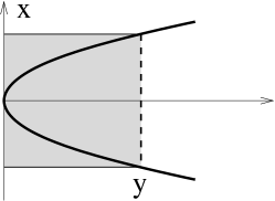
Figure 2: The survival probability for a diffusing particle inside the parabola is approximated as the probability of remaining in the shaded rectangle and exiting along the dashed line.

Let us try to understand the asymptotic (2) heuristically. To this end we construct an extreme statistics argument akin to that popularized in the physics literature by its application to the random trapping problem BV ; GP82 (see L64 ; KRB10 for reviews). We make the assertion that the asymptotic survival probability is controlled by the probability that the particle wanders within the shaded rectangle of Fig. 2 and eventually exits this rectangle only along the dashed boundary. The probability for the particle to remain inside the interval $(-x,x)$ scales as

$$\exp\!\left[-\pi^{2}\,\frac{Dt}{(2x)^{2}}\right]\,.$$

Similarly, the probability for a particle to have longitudinal coordinate $\geq y$, with $y\gg\sqrt{t}$, is governed by the factor

$$\exp\!\left[-\frac{y^{2}}{4Dt}\right]\,.$$

For a particle with longitudinal coordinate $\geq y$, it will survive if its transverse coordinate satisfies $|x|<\sqrt{y/a}$. Combining the two factors written above and writing $x=\sqrt{y/a}$, we may write the survival probability as

$$S\lesssim\int_{0}^{\infty}dy\,\exp\!\left[-\frac{y^{2}}{4Dt}-\pi^{2}\,\frac{aDt}{4y}\right]\,.$$ (3)

This expression represents an (asymptotic) upper bound to the true survival probability because the particle may remain inside the rectangle but still leave the parabola.

We now estimate the integral by the Laplace method by finding the maximum of the integrand. This maximum occurs at $y=y_{*}$ which is determined from the condition

$$2\,\frac{y_{*}}{4Dt}=\pi^{2}\,\frac{aDt}{4y_{*}^{2}}\,.$$

Therefore

$$S\lesssim\exp\!\left[-\frac{3}{4}\,\left(\frac{a\pi^{2}}{2}\right)^{2/3}(Dt)^{1/3}\right]\,.$$ (4)

This expression has the correct dependence on $t,D,a$, but the numerical prefactor is incorrect. According to ls , the amplitude is $A_{\text{exact}}=\tfrac{3}{8}\pi^{2}$ when $a=1,D=\tfrac{1}{2}$, while (4) gives $A=\tfrac{3}{8}\pi^{4/3}$. Since $A<A_{\rm exact}$, this argument gives an upper bound for the survival probability, consistent with the approximation underlying our argument.

It is straightforward to extend the reasoning above to non-quadratic parabolas that are defined by $y=a|x|^{p}$, with $p>1$. The counterpart to (3) is now

$$S\sim\int dy\,\exp\!\left[-\frac{y^{2}}{4Dt}-\frac{\pi^{2}Dt}{4}\,\left(\frac{a}{y}\right)^{2/p}\right]\,,$$

from which

$$S\sim\exp\!\left[-\frac{p+1}{4}\,\left(\frac{\pi^{2}a^{2/p}}{p}\right)^{\frac{p}{p+1}}(Dt)^{\frac{p-1}{p+1}}\right]\,.$$ (5)

The extreme statistics approach also works for other infinite convex domains. For example, if

$$y=Le^{(|x|/\ell)^{b}}\,,$$ (6)

then the counterpart of Eq. (3) is

$$S\sim\int dy\,\exp\!\left[-\frac{y^{2}}{4Dt}-\frac{\pi^{2}Dt}{4\ell^{2}}\,\left(\ln\frac{y}{L}\right)^{-2/b}\right]\,,$$

from which we obtain

$$S\sim\exp\!\left[-\frac{\pi^{2}Dt}{4\ell^{2}}\,\left(\ln\frac{Dt}{L\ell}\right)^{-2/b}\right]\,.$$

A natural extension is to higher dimensions. For example, for the non-quadratic paraboloid in $d$ dimensions defined by

$$y=aR^{p},\quad R=\sqrt{x_{1}^{2}+\ldots+x_{d-1}^{2}},\quad p>1\,,$$ (7)

we now obtain

$$S\sim\int_{0}^{\infty}dy\,\exp\!\left[-\frac{y^{2}}{4Dt}-\frac{j_{\delta}^{2}Dt}{R^{2}}\right]\,.$$ (8)

Here $j_{\delta}$ is the first positive zero of the Bessel function $J_{\delta}$, with $\delta=\tfrac{d-3}{2}$. This numerical factor arises from the long-time solution to the diffusion equation inside a $(d-1)$-dimensional sphere of radius $a$ with absorbing boundaries. Finally, we substitute $R=(y/a)^{1/p}$ into the above estimate and compute the dominant contribution to the integral by the Laplace method to obtain

$$S\sim\exp\!\left[-\frac{p+1}{4}\,\left(\frac{4j_{\delta}^{2}\,a^{2/p}}{p}\right)^{\frac{p}{p+1}}(Dt)^{\frac{p-1}{p+1}}\right]\,.$$ (9)

Once again, the heuristic extreme statistics argument reproduces the correct value of the exponent $\sigma=\frac{p-1}{p+1}$ in the stretched exponential bds ; ls , but not the correct amplitude.

III First Passage for diffusion outside a Paraboloid

Let us now study the complementary situation where a diffusing particle starts outside a paraboloid. This problem is reminiscent of diffusion in (almost) free space except for the presence of an excluded half-line. This analogy suggests that there should be a fundamental difference between two and higher dimensions. In two dimensions, the survival probability of a diffusing particle in the presence of a semi-infinite absorbing line decays as $t^{-1/4}$ bk1 ; CR89 . The same time dependence applies for a diffusing particle exterior to a parabola because the width of the parabola is asymptotically negligible in comparison with the longitudinal coordinate. On the other hand, when $d\geq 4$, a diffusing particle survives with positive probability in the presence of an excluded semi-infinite ray that has a non-zero width. The same behavior should also occur when the excluded region is a paraboloid.

The most interesting behavior occurs in three dimensions. We shall see that the survival probability of a diffusing particle in the exterior of the three-dimensional paraboloid decays as

$$S\sim[\ln(a^{2}Dt)]^{-1}\,,$$ (10)

Similarly, for generalized three-dimensional paraboloids defined by Eq. (7), the survival probability has essentially the same form:

$$S\sim[\ln(a^{2/(p-1)}Dt)]^{-1}\,.$$ (11)

To establish (10) and (11), we recall that the survival probability satisfies the diffusion equation sr

$$\frac{\partial S}{\partial t}=D\nabla^{2}S,\quad S|_{\text{boundary}}=0,\quad S|_{t=0}=1\,.$$

To solve this boundary-value problem we employ the powerful yet simple quasi-static approximation RPJ77 ; C87 ; RA90 ; PLK93 . The quasi-static method is based on dropping the time derivative in the diffusion equation and solving the resulting Laplace equation for distances $\leq\sqrt{Dt}$ from the paraboloid and then matching this density to its unperturbed value when the distance equals $\sqrt{Dt}$. This approach is especially useful for simple geometries, such as planar or cylindrical absorbing boundaries.

In the case of the paraboloid, the quasi-static approach requires a bit more effort, as the boundary is not elementary. However, the boundary simplifies in parabolic coordinates, and the convenience of a simple boundary condition offsets the complication of dealing with the Laplace equation in parabolic coordinates. The parabolic coordinates $(\xi,\eta,\phi)$ are related to the Cartesian coordinates through

$$\begin{split}x_{1}&=\sqrt{\xi\eta}\,\cos\phi\,,\\ x_{2}&=\sqrt{\xi\eta}\,\sin\phi\,,\\ y&=\tfrac{1}{2}(\xi-\eta)\,.\end{split}$$ (12)

with $\xi\geq 0,\eta\geq 0$ and $0\leq\phi\leq 2\pi$. Here the families of surfaces $\xi=\text{const}$ and $\eta=\text{const}$ are confocal paraboloids whose common focus is the origin.

In parabolic coordinates, the Laplacian is

$$\nabla^{2}=\frac{4}{\xi+\eta}\left[\frac{\partial}{\partial\xi}\left(\xi\,\frac{\partial}{\partial\xi}\right)+\frac{\partial}{\partial\eta}\left(\eta\,\frac{\partial}{\partial\eta}\right)\right]+\frac{1}{\xi\eta}\,\frac{\partial^{2}}{\partial\phi^{2}}\,,$$

and we wish to solve the Laplace equation $\nabla^{2}S=0$ in this coordinate system. The solution has axial symmetry $S=S(\xi,\eta)$. By defining the paraboloid in the form $\xi=\xi_{0}$, the boundary condition $S(\xi_{0},\eta)=0$ suggests seeking a solution as a function of $\xi$ alone, $S=S(\xi)$. For this choice the Laplace equation $\nabla^{2}S=0$ reduces to

$$\frac{d}{d\xi}\left(\xi\,\frac{dS}{d\xi}\right)=0\,,$$

whose solution is $S=C\ln(\xi/\xi_{0})$. Matching this solution to the initial density at $\xi\sim\sqrt{Dt}$ fixes the constant and the full solution is

$$S=\frac{\ln(\xi/\xi_{0})}{\ln(\sqrt{Dt}/\xi_{0})}\,.$$ (13)

(As in other applications of the quasi-static approach, the ‘constant’ $C$ is actually time dependent.)  If the diffusing particle starts not far from the apex of the parabola, $\xi\sim\xi_{0}$, the survival probability (13) becomes $S\sim[\ln(Dt/\xi_{0}^{2})]^{-1}$, thereby establishing (10).

Alternatively, Eq. (10) may be inferred from the well-known survival probability of a diffusing particle exterior to an absorbing circle in two dimensions w ; sr . As long as the diffusing particle remains in the half-space $y>0$, the absorbing boundary is a circle that represents the two-dimensional projection of the absorbing parabola. The radius of the circle is not fixed, but rather varies in time as $R\sim\sqrt{y}\sim t^{1/4}$. However, this slower than diffusive variation in the radius does not affect the asymptotics of the survival probability. This same approach applies to the non-quadratic parabola $y=aR^{p}$. The only new feature is that the amplitude $a$ appears as $a^{2/(p-1)}$; this dependence is mandated by dimensional analysis. In this way we also establish Eq. (11).

When $d>3$, we use the $d-$dimensional generalization of parabolic coordinates $(\xi,\eta,\phi_{1},\ldots,\phi_{d-2})$ in which the angular coordinates $(\phi_{1},\ldots,\phi_{d-2})$ are the same as those for spherical coordinates in $d-1$ spatial dimensions. For example, in four dimensions

$$\begin{split}x_{1}&=\sqrt{\xi\eta}\,\cos\phi_{1}\,,\\ x_{2}&=\sqrt{\xi\eta}\,\sin\phi_{1}\cos\phi_{2}\,,\\ x_{3}&=\sqrt{\xi\eta}\,\sin\phi_{1}\sin\phi_{2}\,,\\ y&=\tfrac{1}{2}(\xi-\eta)\,.\end{split}$$

where again $\xi\geq 0,\eta\geq 0$ and the angular coordinates vary in the range $0\leq\phi_{1}\leq\pi$ and $0\leq\phi_{2}\leq 2\pi$.

The Laplacian in $d$-dimensional parabolic coordinates is

$$\nabla^{2}\!=\!\frac{4}{\xi\!+\!\eta}\left[\frac{1}{\xi^{\delta}}\,\frac{\partial}{\partial\xi}\left(\!\xi^{1+\delta}\frac{\partial}{\partial\xi}\!\right)+\frac{1}{\eta^{\delta}}\,\frac{\partial}{\partial\eta}\left(\!\eta^{1+\delta}\frac{\partial}{\partial\eta}\!\right)\right]+\frac{\mathcal{L}}{\xi\eta}\,,$$

where $\mathcal{L}$ is the angular part of the Laplacian in $d-1$ spatial dimensions and we again use the notation $\delta=\frac{d-3}{2}$. Since the problem is axisymmetric, the solution is independent of the angular coordinates and additionally the survival probability depends only on $\xi$. In this case, the Laplace equation $\nabla^{2}S=0$ reduces to

$$\frac{d}{d\xi}\left(\xi^{1+\delta}\frac{dS}{d\xi}\right)=0\,,$$

whose solution is

$$S=1-\left(\frac{\xi_{0}}{\xi}\right)^{\delta}\,.$$ (14)

Therefore instead of decaying to zero, the survival probability remains finite.

Summarizing, we have

$$S\sim\begin{cases}t^{-1/4}&d=2\,,\\ (\ln t)^{-1}&d=3\,,\\ \text{finite}&d\geq 4\,.\end{cases}$$ (15)

The qualitative behavior (15) clearly continues to hold for the generalized paraboloids (7).

IV First Passage Time

For a finite domain, and for various infinite domains such as paraboloids, a diffusing particle is certain to reach the boundary, and its average hitting time is finite. For a diffusing particle inside such a domain, the hitting time $t=t(x,y)$ is a random variable; here $(x,y)$ denotes the starting position of the particle. The hitting time $T(x,y)=\langle t(x,y)\rangle$ averaged over all trajectories that start from $(x,y)$ satisfies the Poisson equation sr ; KRB10

$$D\nabla^{2}T=-1,\quad T|_{\text{boundary}}=0\,.$$ (16)

Let us first determine the exit time for a diffusing particle inside the parabola $y=ax^{2}$. Setting $a=1$ we must solve $D\nabla^{2}T=-1$ subject to the boundary condition $T=0$ when $y=x^{2}$. It is natural to choose $C(y-x^{2})$ as a trial solution, as this function automatically obeys the adsorbing boundary condition and is positive (when $C>0$) inside the parabola. Substituting this trial function into (16) we find that it represents a solution when $C=(2D)^{-1}$. Therefore

$$D\,T=\frac{1}{2}(y-x^{2})\,.$$ (17)

This Laplacian formalism can be straightforwardly extended to determine the higher moments of the hitting time. For example, to determine the second moment $T_{2}=\langle t(x,y)^{2}\rangle$ we must solve the boundary-value problem sr

$$D\nabla^{2}T_{2}=-2T;\qquad T_{2}=0\quad\text{when}\quad y=x^{2}$$ (18)

The form of the solution (17) for the first moment suggests trying a polynomial solution that is divisible by $y-x^{2}$. By trial and error, the appropriate form of $T_{2}$ is

$$T_{2}=A(y-x^{2})^{2}+By(y-x^{2})+C(y-x^{2})\,.$$

Substituting this ansatz into (18) fixes the constants $A,B,C$ and we obtain

$$DT_{2}=\tfrac{1}{12}(y-x^{2})^{2}+\tfrac{1}{3}y(y-x^{2})+\tfrac{5}{12}(y-x^{2})\,.$$ (19)

As might be expected, the second moment of the hitting time scales as the square of the first moment.

For the $d-$dimensional paraboloid defined by the equation $y=R^{2}\equiv x_{1}^{2}+\ldots+x_{d-1}^{2}$, the corresponding results for the average hitting time and the second moment are

$$\begin{split}T&=\frac{y-R^{2}}{2(d-1)D}\,,\\ T_{2}&=\frac{y-R^{2}}{D(d^{2}\!-\!1)}\left[\left(\frac{3}{4}\!+\!\frac{1}{d}\right)y\!-\!\frac{1}{4}\,R^{2}+\frac{3d\!+\!4}{2d^{2}}\right]\,.\end{split}$$ (20)

V The closest particle

Suppose that an infinite absorbing paraboloidal domain initially contains a constant density $\rho$ of non-interacting diffusing particles. As the particles diffuse, the density near the boundary of the paraboloid is depleted. For particles that have not yet been absorbed, a natural way to characterize their spatial distribution is by the distance between the paraboloid and the closest particle. For the paraboloidal geometry, there are two natural (and distinct) definitions of closest particle (Fig. 3):

• the closest particle to the apex of the paraboloid, with corresponding distance $\ell$;

• far from the apex, the closest particle to the side of the paraboloid (distance $b$ in Fig. 3) is a natural measure of the depletion of the density.

Figure 3: Definition of the closest distances $\ell$ and $b$ for an initially constant density of diffusing particles inside an absorbing parabola.

To provide context for these quantities, let us recall basic features of the corresponding problem for the simplest geometry of a constant density of diffusing particles, with an absorbing spherical trap of finite radius $a$ at the origin. For this system, the distance $\ell$ to the closest diffusing particle has the following time dependences W89 ; RA90

$$\ell\sim\begin{cases}(Dt/\rho^{2})^{1/4}&d=1\,,\\ \sqrt{\ln(Dt/a^{2})/(2\pi\rho)}&d=2\,,\\ \textrm{const.}&d>2\,.\end{cases}$$ (21)

Strikingly, the interaction between diffusion and absorption leads to a new length scale $\ell$ that has a non-trivial time dependence and different behavior as function of the spatial dimension. Here we compute the corresponding properties for diffusing particles inside a paraboloidal absorbing boundary.

V.1 Cones

For circular cones, the asymptotics of the density distribution are known, so that the closest particle problem admits an analytical solution.

V.1.1 Wedge

In two dimensions, the circular cone reduces to the wedge. Let $\alpha$ be the angle between the axis of the wedge and its surface. Part of the reason for first studying this system is that the limits of a narrow and a wide wedge provide the asymptotics for the distance between the closest particle and the apex of the parabola, both when the particle is inside or outside the parabola.

Asymptotically, the density of surviving particles is given by bk1 ; CJ59

$$\rho\left(\frac{r^{2}}{Dt}\right)^{\beta}\psi(\theta)\,,$$ (22)

where $(r,\theta)$ are polar coordinates with the origin at the apex and with $\theta=0$ corresponding to the symmetry axis of the wedge. The angular dependence of the density is $\psi(\theta)=\cos\tfrac{\pi\theta}{2\alpha}$ and the survival probability decays as $S\sim t^{-\beta}$, with exponent $\beta=\tfrac{\pi}{4\alpha}$.

To estimate the distance $\ell\/$ from the apex of the wedge to the closest surviving particle we use the extreme statistics criterion KRB10

$$\int_{0}^{\ell}r\,dr\int_{-\alpha}^{\alpha}d\theta\,\rho\left(\frac{r^{2}}{Dt}\right)^{\beta}\psi(\theta)\sim 1\,.$$ (23)

Namely, there should be a single particle inside a pie-shaped sector of length $\ell$ whose center is at the wedge apex. Computing the integral we obtain

$$\ell\sim(Dt)^{\pi/(2\pi+8\alpha)}\,\rho^{-2\alpha/(\pi+4\alpha)}\,.$$ (24)

Some interesting special cases are:

$$\ell\sim\begin{cases}(Dt)^{1/2}&\alpha\downarrow 0\,,\\ (Dt)^{1/4}\,\rho^{-1/4}&\alpha=\pi/4\,,\\ (Dt)^{1/6}\,\rho^{-1/3}&\alpha=\pi/2\,,\\ (Dt)^{1/10}\,\rho^{-2/5}&\alpha=\pi\,.\end{cases}$$ (25)

As the wedge becomes more open, it presents less of a “hazard” to diffusing particles near the apex. Thus the time dependence of $\ell$ becomes progressively slower as $\alpha\to\pi$.

V.1.2 Circular cone in $d$ dimensions

For the $d$-dimensional circular cone, the density is still given by Eq. (22), but the angular part of the density is now an associated Legendre function (see, e.g., bk1 ). The criterion (23) generalizes to

$$\int_{0}^{\ell}r^{d-1}\,dr\int_{0}^{\alpha}(\sin\theta)^{d-2}\,d\theta\,\rho\left(\frac{r^{2}}{Dt}\right)^{\beta}\psi(\theta)\sim 1\,,$$ (26)

from which

$$\ell\sim(Dt)^{\frac{\beta}{2\beta+d}}\,\rho^{-\frac{1}{2\beta+d}}\,.$$ (27)

Here, the exponent $\beta$ and the opening angle of the cone $\alpha$ are related by bk1

$$\begin{split}P_{2\beta+\delta}^{\delta}(\cos\alpha)&=0\qquad d\ {\rm odd}\,,\\ Q_{2\beta+\delta}^{\delta}(\cos\alpha)&=0\qquad d\ {\rm even}\,.\end{split}$$ (28)

where $P_{2\beta+\delta}^{\delta}(\mu)$ and $Q_{2\beta+\delta}^{\delta}(\mu)$ are the associated Legendre functions of degree $2\beta+\delta$ and order $\delta$. Thus in general dimensions, the exponent $\beta$ is the root of a transcendental equation (28) that involves the associated Legendre functions. We must choose the smallest such root to ensure $\psi(\theta)>0$ for all $\theta<\alpha$.

In addition to two dimensions (the wedge), simple results arise in four dimensions where

$$\psi_{4}(\theta)=\frac{\sin\left[(2\beta+1)\theta\right]}{\sin\theta}\,,$$

and the boundary condition $\psi(\alpha)=0$ gives bk1

$$\beta_{4}(\alpha)=\frac{\pi-\alpha}{2\alpha}\,.$$ (29)

In four dimensions, Eq. (27) thus reduces to

$$\ell\sim(Dt)^{(\pi-\alpha)/(2\pi+6\alpha)}\,\rho^{-\alpha/(\pi+3\alpha)}\,.$$ (30)

Some interesting special cases are:

$$\ell\sim\begin{cases}(Dt)^{1/2}&\alpha\downarrow 0\,,\\ (Dt)^{3/14}\,\rho^{-1/7}&\alpha=\pi/4\,,\\ (Dt)^{1/10}\,\rho^{-1/5}&\alpha=\pi/2\,,\\ \rho^{-1/4}&\alpha=\pi\,.\end{cases}$$ (31)

For general spatial dimension, the corresponding results are:

$$\ell\sim\begin{cases}(Dt)^{1/2}&\alpha\downarrow 0\,,\\ (Dt/\rho)^{1/(2+d)}&\alpha=\cos^{-1}(1/\sqrt{d})\,,\\ (Dt/\rho^{2})^{1/(2+2d)}&\alpha=\pi/2\,,\\ \rho^{-1/d}&\alpha=\pi~{}~{}(d\geq 3)\,.\end{cases}$$ (32)

Each of these cases has an interesting interpretation. For a very narrow cone ($\alpha\downarrow 0$), the distance to the closest particle grows diffusively, as $t^{1/2}$. However, density dependence (Eqs. (27) and (30)) leads to a divergent prefactor as $\alpha\downarrow 0$. The case $\alpha=\cos^{-1}(1/\sqrt{d})$ corresponds to survival exponent $\beta=1$ bk1 , that separates the regimes where the average survival time is either finite (for $\alpha<\cos^{-1}(1/\sqrt{d})$ or divergent. The case $\alpha=\pi/2$ corresponds to an absorbing plane, and the behavior of $\ell$ can be simply inferred from the criterion that there should be a single particle within a hemispherical domain of radius $\ell$ about a point on the boundary. Since the density profile is a linear function of distance to the boundary, this calculation is trivial. Finally, when the cone becomes the half-line ($\alpha=\pi$), there is a non-zero survival probability and the distance between the closest particle and the apex merely reduces to the average distance between particles.

V.2 Paraboloids

Let us now analyze the distance between the closest surviving diffusing particle and the origin of a $d$-dimensional paraboloid.

V.2.1 Particles inside the paraboloid

Using the results for the circular cones, and taking the $\alpha\to 0$ limit, gives the universal growth law

$$\ell\sim\sqrt{Dt}\,.$$ (33)

This prediction is valid in arbitrary dimension for all paraboloids, both quadratic and higher order, as in (7).

V.2.2 Particles outside the paraboloid

For the complementary situation where particles are uniformly distributed outside an absorbing paraboloid, it is natural to adopt the results for the circular cones in the $\alpha\to\pi$ limit. This gives

$$\ell\sim\begin{cases}(Dt)^{1/10}\,\rho^{-2/5}&d=2\,,\\ \rho^{-1/d}&d\geq 3\,.\end{cases}$$ (34)

In two dimensions, $\ell$ slowly increases with time, a result that continues to hold even for generalized parabolas (7). In three dimensions, however, the behavior is more subtle because of the ultra-slow logarithmic decay of the survival probability with time (see Eqs. (10) and (11)). To investigate this case, we use the quasi-static result (13) for the density,

$$\rho\,\frac{\ln(\xi/\xi_{0})}{\ln(\sqrt{Dt}/\xi_{0})}\,,$$

and estimate the closest particle distance $\ell$ from the extreme statistics criterion

$$\int_{\xi_{0}}^{\ell}d\xi\int_{0}^{\ell}d\eta\int_{0}^{2\pi}d\phi\,\,\frac{\xi+\eta}{4}\,\rho\,\frac{\ln(\xi/\xi_{0})}{\ln(\sqrt{Dt}/\xi_{0})}\sim 1\,,$$

where $\tfrac{1}{4}(\xi+\eta)d\xi\,d\eta\,d\phi$ is the volume element in parabolic coordinates. Computing the integral we find

$$\frac{\rho\ell^{3}\,\ln(\ell/\xi_{0})}{\ln\tau}\sim 1\,,\qquad\tau=\frac{Dt}{\xi_{0}^{2}}$$

Hence the leading asymptotic is

$$\ell\sim\left[\frac{\rho^{-1}\,\ln\tau}{\ln(\rho^{-1}\xi_{0}^{-3}\ln\tau)}\right]^{1/3}\,.$$ (35)

When $d\geq 4$, the density remains finite and essentially uniform, as particle depletion occurs only over distances of the order of $\xi_{0}$ (see Eq. (14)). Thus if the initial density is low, $\rho\xi_{0}^{d}\ll 1$, the distance between the closest particle and the apex remains of the order of $\rho^{-1/d}$, in agreement with the naive prediction of Eq. (34). Summarizing,

$$\ell\sim\begin{cases}(Dt)^{1/10}\,\rho^{-2/5}&d=2\,,\\ (\ln\tau)^{1/3}\,[\rho\ln(\rho^{-1}\xi_{0}^{-3}\ln\tau)]^{-1/3}&d=3\,,\\ \rho^{-1/d}&d\geq 4\,.\end{cases}$$ (36)

As indicated by Fig. 3, there are two natural measures of closest distance, both of which are needed to characterize the outer envelope of the spatial distribution of surviving particles. Very far away from the apex of the absorbing paraboloid, namely, for distances much greater than $\ell$, the paraboloid is locally planar. In this limit, the distance to the closest particle, defined as $b$ in Fig. 3, is given by the third line of Eq. (32). Thus for the specific case of the parabola ($d=2$), we have

$$\ell\sim(Dt/\rho^{4})^{1/10}\,,\qquad\qquad b\sim(Dt/\rho^{2})^{1/6}\,.$$

These two distances help characterize the spatial distribution of surviving particles without requiring the full solution of the diffusion equation.

VI Discussion

The first-passage properties of a diffusing particle inside an absorbing paraboloid represents a natural and phenomenologically rich extension to the first-passage properties inside an absorbing cone. For the conical system, the survival probability $S(t)$ generally decays as a non-universal power law in time and a basic question, now largely settled bk1 , has been to compute the exponent of this power law as a function of the cone angle and spatial dimension. An intuitive way to understand why there should be a non-universal power-law decay is to decompose the diffusive motion longitudinally and transversely. Longitudinally, a diffusing particle wanders a distance $y\sim\sqrt{t}$ in a time $t$. At this elevation, the transverse distance to the boundaries is $x=y\cot\alpha$ which is also growing as $\sqrt{t}$. This physical picture leads to a survival probability that has a non-universal power-law time dependence kr .

For the paraboloid defined by $y=aR^{p}$, where $R$ is the transverse radius (Eq. (7)), the same decomposition of the motion into longitudinal and transverse components shows that the range of the transverse interval now grows more slowly than $\sqrt{t}$. The feature leads to a more rapid than power-law decay of the survival probability as a function of time. Making use of this decomposition, we constructed an extreme statistics argument that predicted $\ln S\sim-t^{\frac{p-1}{p+1}}$. The exponent value agrees with rigorous bounds and calculations bds ; ls ; we explained how to deduce this result with little effort.

We also studied the mean time until trapping inside the paraboloid $y=aR^{2}$. This mean time, as well as all higher moments, are finite, in distinction to the corresponding behavior inside an absorbing cone. As is naturally expected, the trapping time for a diffusing particle that starts at a given point inside the paraboloid increases as the square of the distance to the closest point on the paraboloidal surface. There are two natural extensions of this computation that have not yet been done: calculating the mean time until trapping inside non-quadratic paraboloids and determining the full distribution of trapping times. To the best of our knowledge this distribution has not been computed even for circular cones.

Finally, we investigated the time dependence of the distance $\ell$ between the apex of an absorbing cone and the closest particle for an initially uniform particle distribution. We found the $\ell$ increases as a power-law in time, with exponent that depends on the wedge opening angle. The increase in this minimum distance becomes extremely slow as the wedge opens up into an excluded half line in two dimensions. In contrast, in three dimensions, the closest distance to an excluded half line increases only logarithmically with time. These latter behaviors were exploited to determine the closest distance between the apex of an absorbing paraboloid and surviving diffusing particles.

- (1) W. Feller, An Introduction to Probability Theory and Its Applications, vol. I (Wiley, New York, 1968).
- (2) H. C. Berg, Random Walks in Biology (Princeton University Press, Princeton, 1983).
- (3) G. H. Weiss, Aspects and Applications of the Random Walk (North-Holland, Amsterdam, 1994).
- (4) J. Rudnick and G. Gaspari, Elements of the Random Walk: An Introduction for Advanced Students and Researchers (Cambridge University, Press, New York, 2004).
- (5) S. Redner, A Guide to First-Passage Processes (Cambridge University Press, New York, 2001).
- (6) M. E. Fisher, J. Stat. Phys. 34, 667 (1984); D. A. Huse and M. E. Fisher, Phys. Rev. B 29, 239 (1984).
- (7) D. ben-Avraham, J. Chem. Phys. 88, 941 (1988).
- (8) M. E. Fisher and M. P. Gelfand, J. Stat. Phys. 53, 175 (1988).
- (9) P. L. Krapivsky and S. Redner, J. Phys. A 29, 5347 (1996); S. Redner and P. L. Krapivsky, Amer. J. Phys. 67, 1277 (1999); D. ben-Avraham, B. M. Johnson, C. A. Monaco, P. L. Krapivsky, and S. Redner, J. Phys. A 36, 1789 (2003).
- (10) J. Cardy and M. Katori, J. Phys. A 36, 609 (2003).
- (11) E. Ben-Naim and P. L. Krapivsky, arXiv:1009.0238.
- (12) E. Ben-Naim and P. L. Krapivsky, arXiv:1009.0239.
- (13) H. Niederhausen, Eur. J. Combinatorics 4, 161 (1983).
- (14) M. Bramson and D. Griffeath, in: Random Walks, Brownian Motion, and Interacting Particle Systems: A Festshrift in Honor of Frank Spitzer, eds. R. Durrett and H. Kesten (Birkhäuser, Boston, 1991).
- (15) R. D. DeBlassie, Probab. Theory Relat. Fields 74, 1 (1987); Probab. Theory Relat. Fields 79, 95 (1988).
- (16) B. Davis and B. Zhang, Proc. Amer. Math. Soc. 121, 925 (1994).
- (17) R. Bañuelos and R. G. Smiths, Probab. Theory Relat. Fields 108, 299 (1997).
- (18) D. J. Grabiner, Ann. Inst. Poincare: Prob. Stat. 35, 177 (1999).
- (19) R. Bañuelos and R. D. DeBlassie, Stoch. Proc. Appl. 116, 36 (2006).
- (20) N. Th. Varopoulos, Math. Proc. Camb. Phil. Soc. 125, 335 (1999); Math. Proc. Camb. Phil. Soc. 129, 301 (1999).
- (21) R. Bañuelos, R. D. DeBlassie, and R. G. Smiths, Ann. Probab. 29, 882 (2001).
- (22) M. Lifshits and Z. Shi, Bernoulli 8, 745 (2002).
- (23) The precise location of the starting point does not affect the most interesting asymptotic behaviors.
- (24) B. Ya. Balagurov and V. G. Vaks, Sov. Phys. JETP 38, 968 (1974).
- (25) P. Grassberger and I. Procaccia, J. Chem. Phys. 77, 6281 (1982).
- (26) M. Lifshits, S. A. Gredeskul, and L. A. Pastur, Introduction to the Theory of Disordered Systems (Wiley, New York, 1988).
- (27) P. L. Krapivsky, S. Redner, and E. Ben-Naim, A Kinetic View of Statistical Physics (Cambridge University Press, Cambridge, 2010).
- (28) D. Considine and S. Redner, J. Phys. A 22, 1621 (1989).
- (29) J. Crank, Free and Moving Boundary Problems (Oxford University Press, New York, 1987).
- (30) H. Reiss, J. R. Patel, and K. A. Jackson, J. Appl. Phys. 48, 5274 (1977).
- (31) S. Redner and D. ben-Avraham, J. Phys. A 23, L1169 (1990).
- (32) P. L. Krapivsky, Phys. Rev. E 47, 1199 (1993).
- (33) G. H. Weiss, S. Havlin, and R. Kopelman, Phys. Rev. A 39, 466 (1989); D. ben-Avraham and G. H. Weiss, Phys. Rev. A 39, 6436 (1989).
- (34) H. S. Carslaw and J. C. Jaeger, Conduction of Heat in Solids (Oxford University Press, Oxford, 1959).