Bayesian Adaptive Lasso

Abstract

We propose the Bayesian adaptive Lasso (BaLasso) for variable selection and coefficient estimation in linear regression. The BaLasso is adaptive to the signal level by adopting different shrinkage for different coefficients. Furthermore, we provide a model selection machinery for the BaLasso by assessing the posterior conditional mode estimates, motivated by the hierarchical Bayesian interpretation of the Lasso. Our formulation also permits prediction using a model averaging strategy. We discuss other variants of this new approach and provide a unified framework for variable selection using flexible penalties. Empirical evidence of the attractiveness of the method is demonstrated via extensive simulation studies and data analysis.

KEY WORDS: Bayesian Lasso; Gibbs sampler; Irrepresentable conditions; Lasso; Scale mixture of normals; Variable Selection

1 Introduction

Consider the linear regression problem

$$y=\mu 1_{n}+X\beta+\epsilon,$$

where $y$ is an $n\times 1$ vector of responses, $X$ is an $n\times p$ matrix of covariates and $\epsilon$ is an $n\times 1$ vector of iid normal errors with mean zero and variance $\sigma^{2}$. As is usual in regression analysis, our major interests are to estimate $\beta=(\beta_{1},...,\beta_{p})^{\prime}$, to identify its important covariates and to make accurate predictions. Without loss of generality, we assume $y$ and $X$ are centered so that $\mu$ is zero and can be omitted from the model.

In an important paper, Tibshirani (1996) proposed the least absolute shrinkage and selection operator (Lasso) for simultaneous variable selection and parameter estimation. The Lasso, formulated in the penalized likelihood framework, minimizes the residual sum of squares with a constraint on the $\ell_{1}$ norm of $\beta$. Formally, the Lasso solves

$$\underset{\beta}{\mbox{min}}~{}(y-X\beta)^{T}(y-X\beta)+\lambda\sum_{j=1}^{p}|\beta_{j}|,$$ (1)

where $\lambda>0$ is the tuning parameter controlling the amount of penalty. The least angle regression (LARS) algorithm provides fast implementation of the Lasso solution (Efron et al.,, 2004; Osborne et al.,, 2000). Furthermore, the Lasso can be model selection consistent provided that the so-called irrepresentable condition on the design matrix is satisfied and that $\lambda$ is chosen judiciously (Zhao and Yu,, 2006).

However, if this condition does not hold, Zou (2006) and Zhao and Yu (2006) showed that the Lasso chooses the wrong model with non-vanishing probability, regardless of the sample size and how $\lambda$ is chosen. The condition is almost necessary and sufficient for model selection consistency of Lasso, which requires that the predictors not in the model are not representable by predictors in the true model. This condition can be easily violated due to the collinearity between the predictors. To address this issue, Zou (2006) and Wang et al. (2006) proposed to use adaptive Lasso (aLasso) which gives consistent model selection. The final inference procedure, thereafter, is based on a single selected model. This may bring undesirable risk properties as discussed by Pötscher and Leeb, (2009). Meinshausen and Buhlmann, (2009) introduced sub-sampling in model selection that improves the Lasso.

The Lasso estimator can be interpreted as the posterior mode using normal likelihood and iid Laplace prior for $\beta$ (Tibshirani, 1996). Yuan and Lin (2006) studied an empirical Bayes variable selection method targeting at finding this mode. The first explicit treatment of the Bayesian Lasso (BLasso), which exploits model inference via posterior distributions, has been proposed by Park and Casella (2008). Hans (2010) considers a formal Bayesian approach to exploring model uncertainty with lasso type priors on parameters in submodels. Griffin and Brown (2010) have previously considered generalizing the Bayesian lasso in various ways including the use of separate scale parameters for different coefficients in the Laplace prior with gamma mixing distributions for the scale parameters. This is similar to the priors we use here, but Griffin and Brown (2010) focused on finding posterior mode estimates via an EM algorithm whereas our objectives here are somewhat broader. In particular we aim to investigate MCMC computational methods for these priors, estimates of regression coefficients other than the mode, different choices for smoothing parameters, model averaging strategies which explore model uncertainty for predictive purposes and generalizations beyond the linear model.

Although the Lasso was originally designed for variable selection, the BLasso loses this attractive property, not setting any of the coefficients to zero. A post hoc thresholding rule may overcome this difficulty but it brings the problem of threshold selection. Alternatively, Kyung et al. (2009) recommended to use the credible interval on the posterior mean. Although it gives variable selection, this suggestion fails to explore the uncertainty in the model space. On the other hand, the so-called spike and slab prior, in which the scale parameter for a coefficient is a mixture of a point mass at zero and a proper density function such as normal or double exponential (Yuan and Lin, 2005), allows exploration of model space at the expense of increased computation for a full Bayesian posterior.

This work is motivated by the need to explore model uncertainty and to achieve parsimony. With these objectives, we consider the following adaptive Lasso estimator:

$$\underset{\beta}{\mbox{min}}~{}(y-X\beta)^{T}(y-X\beta)+\sum_{j=1}^{p}\lambda_{j}|\beta_{j}|,$$ (2)

where different penalty parameters are used for the regression coefficients. Naturally, for the unimportant covariates, we should put larger penalty parameters $\lambda_{j}$ on their corresponding coefficients. This strategy was proposed by Zou (2006) and Wang et al. (2006) by using some preliminary estimates of $\beta$ such as the least-squares estimate $\hat{\beta}^{0}$ and modifying $\lambda_{j}$ as $\lambda/|\hat{\beta}_{j}^{0}|$. Our treatment is completely different and is motivated by the following arguments. Suppose tentatively that we have a posterior distribution on $\{\lambda_{j}\}_{j=1}^{p}$. By drawing random samples from this distribution and plugging these into (2), we can solve for $\beta$ using fast algorithms developed for Lasso (Efron et al., 2004; Figueiredo et al., 2007) and subsequently obtain an array of (sparse) models. These models can be used not only for exploring model uncertainty, but also for prediction with a variety of methods akin to Bayesian model averaging. Since there are $p$ tuning parameters, a hierarchical model is proposed to alleviate the problem of estimating many parameters. We develop an efficient Gibbs sampler for posterior inference.

The BaLasso permits a unified treatment for variable selection with flexible penalties, using the least sqaures approximation (Wang and leng, 2007). The extension encompasses generalized linear models, Cox’s model and other parametric models as special cases. We outline novel applications of BaLasso when structured penalties are present, for example, grouped variable selection (Yuan and Lin, 2007) and variable selection with a prior hierarchical structure (Zhao, Rocha and Yu, 2009).

The rest of the paper is organized as follows. The Bayesian adaptive Lasso (BaLasso) method is presented in Section 2. Furthermore, we propose two approaches for estimating the tuning parameter vector $\lambda=(\lambda_{1},...,\lambda_{p})^{\prime}$ and give an explanation for the shrinkage adaptivity. Section 3 discusses model selection and Bayesian model averaging. In Section 4, the finite sample performance of BaLasso is illustrated via simulation studies, and analysis of two real datasets. Section 5 presents a unified framework which deals with variable selection in models with structured penalties. Section 6 gives concluding remarks. A Matlab implementation is available from the authors’ homepage. The software is very general and deals with many parametric models encountered in practice.

2 Bayesian Adaptive Lasso

The $\ell_{1}$ penalty corresponds to a conditional Laplace prior (Tibshirani, 1996) as

$$\pi(\beta|\sigma^{2})=\prod_{j=1}^{p}\frac{\lambda}{2\sqrt{\sigma^{2}}}e^{-\lambda|\beta_{j}|/\sqrt{\sigma^{2}}},$$

which can be represented as a scale mixture of normals with an exponential mixing density (Andrews and Mallows, 1974)

$$\frac{\lambda}{2}e^{-\lambda|z|}=\int_{0}^{\infty}\frac{1}{\sqrt{2\pi s}}e^{-z^{2}/(2s)}\frac{\lambda^{2}}{2}e^{-\lambda^{2}z/2}ds.$$

This motivates the following hierarchical BLasso model (Park and Casella,, 2008)

$$y|X,\beta,\sigma^{2} \sim N_{n}(X\beta,\sigma^{2}I_{n})$$

$$\beta|\sigma^{2},\tau_{1}^{2},...,\tau_{p}^{2} \sim N_{p}(0_{p},\sigma^{2}D_{\tau})$$ (3)

$$D_{\tau} = \mbox{diag}(\tau_{1}^{2},...,\tau_{p}^{2})$$

with the following priors on $\sigma^{2}$ and $\tau=(\tau_{1}^{2},...,\tau_{p}^{2})$:

$$\sigma^{2},\tau_{1}^{2},...,\tau_{p}^{2}\sim\pi(\sigma^{2})d\sigma^{2}\prod_{j=1}^{p}\frac{\lambda^{2}}{2}e^{-\lambda^{2}\tau_{j}^{2}/2}d\tau_{j}^{2}$$ (4)

for $\sigma^{2}>0$ and $\tau_{1}^{2},...,\tau_{p}^{2}>0$. Park and Casella, (2008) suggested to use the improper prior $\pi(\sigma^{2})\propto 1/\sigma^{2}$ to model the error variance.

As discussed in the introduction, the Lasso uses the same shrinkage for every coefficient and may not be consistent for certain design matrices in terms of model selection. This motivates us to replace (4) in the hierarchical structure by a more adaptive penalty

$$\sigma^{2},\tau_{1}^{2},...,\tau_{p}^{2}\sim\pi(\sigma^{2})d\sigma^{2}\prod_{j=1}^{p}\frac{\lambda_{j}^{2}}{2}e^{-\lambda_{j}^{2}\tau_{j}^{2}/2}d\tau_{j}^{2}.$$ (5)

The major difference of this formulation is to allow different $\lambda^{2}_{j}$, one for each coefficient. Intuitively, if small penalty is applied to those covariates that are important and large penalty is applied to those which are unimportant, the Lasso estimate, as the posterior mode, can be model selection consistent (Zou, 2006; Wang et al. 2007). Indeed, as we will see in Section 2.2 and in later numerical experiments, in the posterior distribution, the $\lambda_{j}$’s for zero $\beta_{j}$’s will be much larger than those $\lambda_{j}$’s for nonzero $\beta_{j}$’s.

The Gibbs sampling scheme follows Park and Casella (2008). For Bayesian inference, the full conditional distribution of $\beta$ is multivariate normal with mean $A^{-1}X^{T}y$ and variance $\sigma^{2}A^{-1}$, where $A=X^{T}X+D_{\tau}^{-1}$. The full conditional for $\sigma^{2}$ is inverse-gamma with shape parameter $(n-1)/2+p/2$ and scale parameter $(y-X\beta)^{T}(y-X\beta)/2+\beta^{T}D_{\tau}^{-1}\beta/2$ and $\tau_{1}^{2},...,\tau_{p}^{2}$ are conditionally independent, with $1/\tau_{j}^{2}$ conditionally inverse-Gaussian with parameters

$$\tilde{\mu}_{j}=\frac{\lambda_{j}\sigma}{|\beta_{j}|}~{}\text{and}~{}\tilde{\lambda}_{j}=\lambda_{j}^{2}$$

where the inverse-Gaussian density is given by

$$f(x)=\sqrt{\tilde{\lambda}}{2\pi}x^{-3/2}\exp\left\{-\frac{\tilde{\lambda}(x-\tilde{\mu}_{j})^{2}}{2(\tilde{\mu})^{2}x}\right\},~{}x>0.$$

As observed in Park and Casella (2008), the Gibbs sampler with block updating of $\beta$ and $(\tau_{1}^{2},...,\tau_{p}^{2})$ is very fast.

2.1 Choosing the Bayesian Adaptive Lasso Parameters

We discuss two approaches for choosing BaLasso parameters in the Bayesian framework: the empirical Bayes (EB) method and the hierarchical Bayes (HB) approach using hyper-priors. The EB approach aims to estimate the $\lambda_{j}$ via marginal maximum likelihood, while the HB approach uses hyperpriors on the $\lambda_{j}$ which enables posterior inference on these shrinkage parameters.

Empirical Bayes (EB) Estimation. A natural choice is to estimate the hyper-parameters $\lambda_{j}$ by marginal maximum likelihood. However, in our framework, the marginal likelihood for the $\lambda_{j}$s is not available in closed form. To deal with such a problem, Casella, (2001) proposed a multi-step approach based on an EM algorithm with the expectation in the E-step being approximated by the average from the Gibbs sampler. The updating rule then for $\lambda_{j}$ is easily seen to be

$$\lambda_{j}^{(k)}=\sqrt{\dfrac{2}{E_{\lambda_{j}^{(k-1)}}(\tau_{j}^{2}|y)}}$$ (6)

where $\lambda_{j}^{(k)}$ is the estimate of $\lambda_{j}$ at the $k$th stage and the expectation $E_{\lambda_{j}^{(k-1)}}(.)$ is approximated by the average from the Gibbs sampler with the hyper-parameters are set to $\lambda_{j}^{(k-1)}$.

Casella’s method may be computationally expensive because many Gibbs sampler runs are needed. Atchade, (2009) proposed a single-step approach based on stochastic approximation which can obtain the MLE of the hyper-parameters using a single Gibbs sampler run. In our framework, making the transformation $\lambda_{j}=e^{s_{j}}$, the updating rule for the hyper-parameters $s_{j}$ can be seen as (Atchade, 2009, Algorithm 3.1)

$$s_{j}^{(n+1)}=s_{j}^{(n)}+a_{n}(2-e^{2s_{j}^{(n)}}\tau_{n+1,j}^{2})$$

where $s_{j}^{(n)}$ is the value of $s_{j}$ at the $n$th iteration, $\tau_{n,j}^{2}$ is the $n$th Gibbs sample of $\tau_{j}^{2}$, and $\{a_{n}\}$ is a sequence of step-sizes such that

$$a_{n}\searrow 0,\mskip 5.0mu plus 5.0mu\mskip 5.0mu plus 5.0mu\sum a_{n}=\infty,\mskip 5.0mu plus 5.0mu\mskip 5.0mu plus 5.0mu\sum a_{n}^{2}<\infty.$$

In the following simulation, $a_{n}$ is set to $1/n$. Strictly speaking, choosing a proper $a_{n}$ is an important problem of stochastic approximation which is beyond the scope of this paper. In practice, $a_{n}$ is often set after a few trials by justifying the convergence of iterations graphically.

Hierarchical Model. Alternatively, $\lambda_{j}$s themselves can be treated as random variables and join the Gibbs updating by using an appropriate prior on $\lambda_{j}^{2}$. Here for simplicity and numerical tractability, we take the following gamma prior (Park and Casella,, 2008)

$$\pi(\lambda_{j}^{2})=\frac{\delta^{r}}{\Gamma(r)}(\lambda_{j}^{2})^{r-1}e^{-\delta\lambda_{j}^{2}}.$$ (7)

The advantage of using such a prior is that the Gibbs sampling algorithm can be easily implemented. More specifically, when this prior is used, the full conditional of $\lambda_{j}^{2}$ is gamma with shape parameter $1+r$ and rate parameter $\tau_{j}^{2}+\delta$. This specification allows $\lambda_{j}^{2}$ to join the other parameters in the Gibbs sampler. Although the number of the penalty parameters $\lambda_{j}$ has increased to $p$ in BaLasso from a single parameter in Lasso, the fact that the same prior is used on these parameters greatly reduces the degrees of freedom in specifying the prior.

As a first choice, we can fix hyper-parameters $r$ and $\delta$ to some small values in order to get a flat prior. Alternatively, we can fix $r$ and use an empirical Bayes approach where $\delta$ is estimated. The updating rule for $\delta$ (Casella, 2001) can be seen as

$$\delta^{(k)}=\frac{pr}{\sum_{j=1}^{p}E_{\delta^{(k-1)}}(\lambda_{j}^{2}|y)}.$$

Theoretically, we need not worry so much about how to select $r$ because parameters that are deeper in the hierarchy have less effect on inference (Lehmann,, 1998, p.260). In our simulation study and data analysis, we use $r=.1$ which gives a fairly flat prior and stable results.

2.2 Adaptive shrinkage

By allowing different $\lambda_{j}^{2}$, adaptive shrinkage on the coefficients is possible. We demonstrate the adaptivity by a simple simulation in which a data set of size 50 is generated from the model

$$y=\beta_{1}x_{1}+\beta_{2}x_{2}+\sigma\epsilon$$

with $\beta=(3,\ 0)^{\prime},\ \sigma=1,\ \epsilon\sim N(0,1)$.

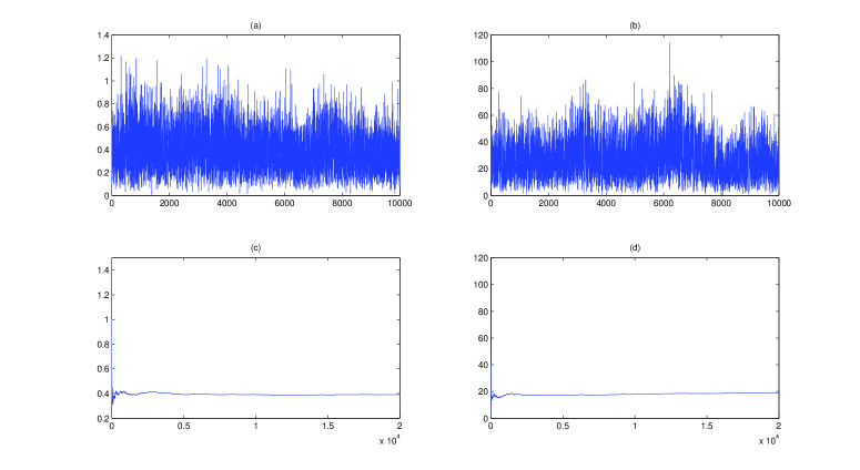
Figure 1: (a)-(b): Gibbs samples for $\lambda_{1}$ and $\lambda_{2}$, respectively. (c)-(d): Trace plot for $\lambda^{(n)}_{1}$ and $\lambda^{(n)}_{2}$ by Atchade’s method.

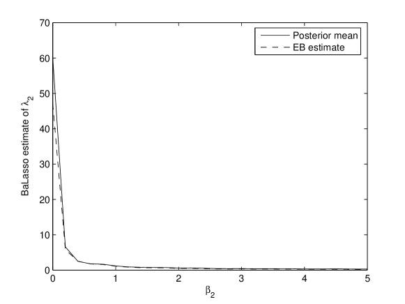
Figure 2: Plots of EB and posterior estimates of $\lambda_{2}$ versus $\beta_{2}$

Because $\beta_{1}\not=0,\ \beta_{2}=0$ we expect that the EB and posterior estimate of $\lambda_{2}$ would be much larger than that of $\lambda_{1}$. As a result, a heavier penalty is put on $\beta_{2}$ such that $\beta_{2}$ is more likely to be shrunken to zero. This phenomenon is demonstrated graphically in Figure 1. Figure 1 (a)-(b) plot 10,000 Gibbs samples (after discarding 10,000 burn-in samples) for $\lambda_{1}$ and $\lambda_{2}$ (not $\lambda_{1}^{2},\ \lambda_{2}^{2}$), respectively. The posterior distribution of $\lambda_{2}$ is central around a value of $22$ which is much larger than .39, the posterior median of $\lambda_{1}$. Figure 1 (c)-(d) shows the trace plots of iterations $\lambda_{1}^{(n)}$, $\lambda_{2}^{(n)}$ from Atchade’s method. Marginal maximum likelihood estimates of $\lambda_{1}$ and $\lambda_{2}$ are 0.39 and 19, respectively. In Figure 2 we plot EB and posterior mean estimates of $\lambda_{2}$ versus $\beta_{2}$ when $\beta_{2}$ varies from 0 to 5. Clearly, both the EB and the posterior estimates of $\lambda_{2}$ decrease as $\beta_{2}$ increases, which demonstrates that lighter penalty is applied for stronger signals.

3 Inference

3.1 Estimation and Model Selection

For the adaptive Lasso, the usual methods to choose the $\lambda_{j}$’s would be computationally demanding. From the Bayesian perspective, one can draw MCMC samples based on BaLasso and get an estimated posterior quantity for $\beta$. Like the original Bayesian Lasso, however, a full posterior exploration gives no sparse models and would fail as a model selection method. Here we take a hybrid Bayesian-frequentist point of view in which coefficient estimation and variable selection are simultaneously conducted by plugging in an estimate of $\lambda$ into (2), where $\lambda$ might be the marginal maximum likelihood estimator, posterior median or posterior mean. Hereafter these suggested strategies are abbreviated as BaLasso-EB, BaLasso-Median, and BaLasso-Mean, respectively.

With the presence of a posterior sample, we also propose another strategy for exploring model uncertainty. Let $\{\lambda^{(s)}\}_{s=1}^{N}$ be Gibbs samples drawn from the hierarchical model (2), (5) and (7). For the $s$th Gibbs sample $\lambda^{(s)}=(\lambda_{1}^{(s)},...,\lambda_{p}^{(s)})^{\prime}$, we plug $\lambda^{(s)}$ into (2) and then record the frequencies of each variable being chosen out of $N$ samples. The final chosen model consists of those variables whose frequencies are not less than 0.5. This strategy will be abbreviated as BaLasso-Freq. The chosen model is somewhat similar in spirit to the so-called median probability (MP) model proposed by Barbieri and Berger, (2004).

As we will see in Section 4, all of our proposed strategies have surprising improvement in terms of variable selection over the original Lasso and the adaptive Lasso.

3.2 A Model Averaging Strategy

When model uncertainty is present, making inferences based on a single model may be dangerous. Using a set of models helps to account for this uncertainty and can provide improved inference. In the Bayesian framework, Bayesian model averaging (BMA) is widely used for prediction. BMA generally provides better predictive performance than a single chosen model, see Raftery et al., (1997); Hoeting et al., (1999) and references therein. For making inference via multiple models, we use the hierarchical model approach for estimating $\lambda$ and refer to the strategy outlined below as BaLasso-BMA. It should be emphasized, however, that our model averaging strategy is unrelated to the usual formal Bayesian treatment of model uncertainty. Rather, our idea is simply to use an ensemble of sparse models for prediction obtained from sampling the posterior distribution of smoothing parameters and considering different sparse conditional mode estimates of regression coefficients for the smoothing parameters so obtained.

Let $\Delta=(x_{\Delta},y_{\Delta})$ be a future observation and $D=(X,y)$ be the past data. The posterior predictive distribution of $\Delta$ is given by

$$p(\Delta|D)=\int p(\Delta|\beta)p(\beta|\lambda,D)d\beta p(\lambda|D)d\lambda.$$ (8)

Suppose that we measure predictive performance via a logarithmic scoring rule (Good,, 1952), i.e., if $g(\Delta|D)$ is some distribution we use for prediction then our predictive performance is measured by $\log g(\Delta|D)$ (where larger is better). Then for any fixed smoothing parameter vector $\lambda_{0}$

$$E(\log p(\Delta|D)-\log p(\Delta|\lambda_{0},D))=\int\log\dfrac{p(\Delta|D)}{p(\Delta|\lambda_{0},D)}p(\Delta|D)d\Delta$$

is nonnegative because the right hand side is the Kullback-Leibler divergence between $p(\Delta|D)$ and $p(\Delta|\lambda_{0},D)$. Hence prediction with $p(\Delta|D)$ is superior in this sense to prediction with $p(\Delta|\lambda_{0},D)$ with any choice of $\lambda_{0}$.

Our hierarchical model (2), (5) and (7) offers a natural way to estimate the predictive distribution (8), in which the integral is approximated by the average from Gibbs samples of $\lambda$. For example, in the case of point prediction for $y_{\Delta}$ with squared error loss, the ideal prediction is

$$E(y_{\Delta}|D)=\int x_{\Delta}^{\prime}E(\beta|\lambda,D)p(\lambda|D)d\lambda=x_{\Delta}^{\prime}E(\beta|D),$$

where $E(\beta|D)$ can be estimated by the mean of Gibbs samples for $\beta$. Write $\hat{\beta}_{\lambda}$ as the conditional posterior mode for $\beta$ given $\lambda$. One could approximate $x_{\Delta}^{\prime}E(\beta|D)$ by replacing $E(\beta|D)$ with the conditional posterior mode $\hat{\beta}_{\hat{\lambda}}$ for some fixed value $\hat{\lambda}$ of $\lambda$. However, this ignores uncertainty in estimating the penalty parameters. An alternative strategy is to replace $E(\beta|D,\lambda)$ in the integral above with $\hat{\beta}_{\lambda}$ and to integrate it out accordingly. This should provide a better approximation to the full Bayes solution than the approach which uses a fixed $\hat{\lambda}$. In fact, we predict $E(y_{\Delta}|D)$ by $s^{-1}\sum_{i=1}^{s}x_{\Delta}^{\prime}\hat{\beta}_{\lambda^{(i)}}$ where $\lambda^{(i)}$, $i=1,...,s$, denote MCMC samples drawn from the posterior distribution of $\lambda$. Note that this approach has advantages in interpretation over the fully Bayes’ solution. By considering the models selected by the conditional posterior mode for different draws of $\lambda$ from $p(\lambda|y)$ we gain an ensemble of sparse models that can be used for interpretation. As will be seen in Section 4, when there is model uncertainty, BaLasso-BMA provides an ensemble of sparse models and may have better predictive performance than conditioning on a single fixed smoothing parameter vector $\lambda$.

4 Examples

In this section we study the proposed methods through numerical examples. These methods are also compared to Lasso, aLasso and BLasso in terms of variable selection and predictions. We use the LARS algorithm of Efron et al., (2004) for Lasso and aLasso in which fivefold cross-validation is used to choose shrinkage parameters. In the adaptive Lasso, we either use the least squares estimate (Example 1 and 2) or the Lasso estimate (Example 3) as the preliminary estimate. For the optimization problem (2), we use the gradient projection algorithm developed by Figueiredo et al., (2007).

4.1 Simulation

Example 1 (Simple example). We simulate data sets from the model

$$y=x^{\prime}\beta+\sigma\epsilon,$$ (9)

where $\beta=(3,\ 1.5,\ 0,\ 0,\ 2,\ 0,\ 0,\ 0)^{\prime}$, $x_{j}$ follows N(0,1) marginally and the correlation between $x_{j}$ and $x_{k}$ is $0.5^{|j-k|}$, and $\epsilon$ is iid N(0,1). We compare the performance of the proposed methods in Section 3.1 to that of the original Lasso and adaptive Lasso. The performance is measured by the frequency of correctly-fitted models over 100 replications. The simulation results are summarized in Table 1 and suggest that the proposed methods perform better than Lasso and aLasso in model selection.

$n$	$\sigma$	Lasso	aLasso	BaLasso-Freq	BaLasso-Median	BaLasso-Mean	BaLasso-EB
30	1	50	71	86	86	97	78
	3	17	8	35	34	18	39
60	1	66	76	81	79	100	83
	3	44	38	54	53	55	46
120	1	73	76	87	87	100	87
	3	58	55	81	81	97	86

Table 1: Frequency of correctly-fitted models over 100 replications for Example 1.

Example 2 (Difficult example). For the second example, we use Example 1 in Zou, (2006), for which the Lasso does not give consistent model selection, regardless of the sample size and how the tuning parameter $\lambda$ is chosen. Here $\beta=(5.6,\ 5.6,\ 5.6,\ 0)^{\prime}$ and the correlation matrix of $x$ is such that $\text{cor}(x_{j},x_{k})=-.39,~{}j<k<4$ and $\text{cor}(x_{j},x_{4})=.23,~{}j<4$.

The experimental results are summarized in Table 2 in which the frequencies of correct selection are shown. We see that the original Lasso does not seem to give consistent model selection. For all the other methods, the frequencies of correct selection go to 1 as $n$ increases and $\sigma$ decreases. In general, our proposed method for model selection performs better than aLasso.

$n$	$\sigma$	Lasso	aLasso	BaLasso-Freq	BaLasso-Median	BaLasso-Mean	BaLasso-EB
60	9	0	5	8	8	9	12
120	5	10	45	66	65	66	51
300	3	12	65	83	83	85	83
300	1	12	100	100	100	100	100

Table 2: Frequency of correctly-fitted models over 100 replications for Example 2.

Example 3 (Large $p$ example). The variable selection problem with large $p$ (even larger than $n$) is recently an active research area. We consider an example of this kind in which $p=100$ with various sample sizes $n=50,\ 100,\ 200$. We set up a sparse recovery problem in which most of coefficients are zero except $\beta_{j}=5,\ j=10,20,...,100$. From the previous examples, the performances of the four methods BaLasso-Freq, BaLasso-Median, BaLaso-Mean and BaLasso-EB are similar. We therefore just consider the BaLasso-Mean as a representative and compare it to the adaptive Lasso which is generally superior to the Lasso.

Table 3 summarizes our simulation results, in which the design matrix is simulated as in Example 1. BaLasso-Mean performs satisfactorily in this example and outperforms aLasso in variable selection.

$n$	$\sigma$	aLasso	BaLasso-Mean
50	1	24	39
	3	24	35
	5	8	29
100	1	40	100
	3	39	99
	5	20	86
200	1	100	100
	3	88	100
	5	78	97

Table 3: Frequency of correctly-fitted models over 100 replications for Example 3.

Example 4 (Prediction). In this example, we examine the predictive ability of BaLasso-BMA experimentally. As discussed in Section 3.2, when there is model uncertainty, making predictions conditioning on a single fixed parameter vector is not optimal predictively. Suppose that the dataset $D$ is split into two sets: a training set $D^{T}$ and prediction set $D^{P}$. Let $\Delta=(x_{\Delta},y_{\Delta})\in D^{P}$ be a future observation and $\hat{y}_{\Delta}$ be a prediction of $y_{\Delta}$ based on $D^{T}$. We measure the predictive performance by the prediction squared error (PSE)

$$\text{PSE}=\dfrac{1}{|D^{P}|}\sum_{\Delta\in D^{P}}|y_{\Delta}-\hat{y}_{\Delta}|^{2}.$$ (10)

We compare PSE of BaLasso-BMA to that of BaLasso-Mean in which $\hat{y}_{\Delta}=x_{\Delta}^{\prime}\hat{\beta}$ where $\hat{\beta}$ is the solution to (2) with smoothing parameter vector fixed at the posterior mean of $\lambda$. We also compare the predictive performance of BaLasso-BMA to that of the Lasso, aLasso, and the original Bayesian Lasso (BLasso). The implementation of BLasso is similar to BaLasso except that BLasso has a single smoothing parameter.

We first consider a small-$p$ case in which data sets are generated from model (9) but now with $\beta=(3,\ 1.5,\ 0.1,\ 0.1,\ 2,\ 0,\ 0,\ 0)^{\prime}$. By adding two small effects we expect there to be model uncertainty. Table 4 presents the prediction squared errors averaged over 100 replications with various factors $n_{T}$ (size of training set), $n_{P}$ (size of prediction set) and $\sigma$. The experiment shows that BaLasso-BMA performs slightly better than BLasso and BaLasso-Mean, and much better than the Lasso and aLasso.

Similarly, we consider a large-$p$ case as in Example 3 but now with $\beta_{10}=\beta_{20}=\beta_{30}=\beta_{40}=\beta_{50}=.5$ in order to get model uncertainty. The results are summarized in Table 5. Unlike for the small-$p$ case, BLasso now performs surprisingly badly. This may be due to the fact that BLasso uses the same shrinkage for every coefficient. As shown, BaLasso-BMA outperforms the others.

$n_{T}=n_{P}$	$\sigma$	Lasso	aLasso	BLasso	BaLasso-Mean	BaLasso-BMA
30	1	2.029	1.976	1.276	1.175	1.165
	3	17.43	17.37	10.88	15.51	11.06
	5	42.74	42.13	29.43	41.32	29.56
	10	126.6	126.2	109.6	123.9	109.9
100	1	1.449	1.436	1.044	1.077	1.032
	3	12.69	12.58	9.662	9.627	9.485
	5	34.89	34.79	25.79	27.55	25.83
	10	117.6	117.5	105.7	118.2	106.5
200	1	1.279	1.274	1.018	1.036	1.014
	3	11.44	11.40	9.424	9.326	9.320
	5	31.30	31.18	25.32	25.36	25.19
	10	120.7	120.7	103.9	108.8	104.3

Table 4: Prediction squared error averaged over 100 replications for the small-$p$ case.

$n_{T}=n_{P}$	$\sigma$	Lasso	aLasso	BLasso	BaLasso-Mean	BaLasso-BMA
100	1	3.501	4.173	9.574	1.673	1.234
	3	15.49	17.70	27.42	10.88	10.42
	5	34.45	39.81	42.43	28.66	28.19
	10	149.3	178.1	161.0	124.5	117.6
200	1	2.468	2.417	5.231	1.110	1.072
	3	17.11	17.09	15.12	10.42	10.22
	5	44.49	44.39	33.92	27.18	27.06
	10	148.1	147.5	136.1	112.0	108.9

Table 5: Prediction squared error averaged over 100 replications for the large-$p$ case.

4.2 Real Examples

Example 5: Body fat data. Percentage of body fat is one important measure of health, which can be accurately estimated by underwater weighing techniques. These techniques often require special equipment and are sometimes not convenient, thus fitting percent body fat to simple body measurements is a convenient way to predict body fat. Johnson, (1996) introduced a data set in which percent body fat and 13 simple body measurements (such as weight, height and abdomen circumference) are recorded for 252 men (see Table 6 for the summarized data). This data set was also carefully analyzed by Hoeting et al., (1999). Following Hoeting et al., we omit the 42nd observation which is considered as an outlier. Previous diagnostic checking (Hoeting et al.,, 1999) showed that it is reasonable to assume a linear regression model.

Predictor number	Predictor	mean	s.d.
$Y$	Percent body fat (%)	18.89	7.72
$X_{1}$	Age (years)	44.89	12.63
$X_{2}$	Weight (pounds)	178.82	29.40
$X_{3}$	Height (inches)	70.31	2.61
$X_{4}$	Neck circumference (cm)	37.99	2.43
$X_{5}$	Chest circumference (cm)	100.80	8.44
$X_{6}$	Abdomen circumference (cm)	92.51	10.78
$X_{7}$	Hip circumference (cm)	99.84	7.11
$X_{8}$	Thigh circumference (cm)	59.36	5.21
$X_{9}$	Knee circumference (cm)	38.57	2.40
$X_{10}$	Ankle circumference (cm)	23.10	1.70
$X_{11}$	Extended biceps circumference	32.27	3.02
$X_{12}$	Forearm circumference (cm)	28.66	2.02
$X_{13}$	Wrist circumference (cm)	18.23	.93

Table 6: Body fat example: summarized data

We first consider the variable selection problem. We center the variables so that the intercept is not considered. Lasso chooses $X_{1},\ X_{2},\ X_{3},\ X_{4},\ X_{6},\ X_{7},\ X_{8},\ X_{11},\ X_{12},\ X_{13}$ in the final model with a BIC value $712.16$, while aLasso has one fewer variable $X_{3}$ with a BIC value $709.46$. BaLasso-Freq, BaLasso-Median, BaLasso-Mean and BaLasso-EB all choose $X_{1},\ X_{2},\ X_{4},\ X_{6},\ X_{8},\ X_{11},\ X_{12},\ X_{13}$, one fewer variable ($X_{7}$) than aLasso. The BIC value for BaLasso is $708.92$, smaller than that of Lasso and aLasso. A simple analysis shows that $X_{3}$ and $X_{7}$ are highly correlated to $X_{6}$ (the correlation coefficients are .89 and .92, respectively). Additionally, $X_{6}$ is the most important predictor (Hoeting et al.,, 1999). Thus removing $X_{3}$ and $X_{7}$ from the model helps to avoid the multicollinearity problem. To conclude, BaLasso chooses the simplest model with the smallest BIC.

Models													PMP (%)
$X_{1}$	$X_{2}$	$X_{3}$	$X_{4}$	$X_{5}$	$X_{6}$	$X_{7}$	$X_{8}$	$X_{9}$	$X_{10}$	$X_{11}$	$X_{12}$	$X_{13}$
1	1	0	1	0	1	0	1	0	0	1	1	1	2.23
1	1	0	0	0	1	0	1	0	0	0	1	1	2.03
1	1	0	0	0	1	0	0	0	0	1	0	1	1.80
0	1	0	0	0	1	0	0	0	0	1	0	1	1.77
1	1	0	1	0	1	0	1	0	0	0	1	1	1.63
1	1	0	1	0	1	0	0	0	0	1	0	1	1.57
1	1	0	1	0	1	1	1	0	0	1	1	1	1.43
0	1	0	1	0	1	0	0	0	0	1	0	1	1.43
0	1	0	0	0	1	0	0	0	0	0	1	1	1.43
0	1	0	0	0	1	0	1	0	0	0	1	1	1.43

Table 7: Body fat example: 10 models with highest posterior model probability

We now proceed to explore model uncertainty inherent in this dataset. Let $M(\lambda)$ be the model selected w.r.t. shrinkage parameter vector $\lambda$. We define the posterior model probability (PMP) of a model $M$ to be

$$p(M|D)=\int_{\lambda:M(\lambda)=M}p(\lambda|D)d\lambda.$$

Note that this is not a posterior model probability in the usual sense in formal Bayesian model comparison, but simply represents the uncertainty of the sparsity structure in the conditional posterior mode estimate induced by the uncertainty in the posterior distribution on the smoothing parameter. From the Gibbs samples of $\lambda$, it is straightforward to estimate these PMPs. Table 7 presents 10 models with highest PMP which indicates high model uncertainty. The model with highest posterior probability and these 10 mostly selected models account for only 2.23% and 16.8% of the total posterior model probability, respectively. With this model uncertainty, using a single model for prediction may be risky.

We now examine the predictive performance of the approaches. To this end, we split the dataset (without standardizing) into two parts: the first 150 observations are used as the training set, the remaining observations are used as the prediction set. The out-of-sample predictive squared errors (PSEs) of aLasso, BaLasso-Mean, BaLasso-Median, BaLasso-EB, BLasso and BaLasso-BMA are 18.92, 18.28, 19.79, 19.00, 18.69, 18.13, respectively. Thus, for this dataset, BaLasso-BMA has the best predictive performance.

Example 6: Prostate cancer data. Stamey et al. (1989) studied the correlation between the level of prostate antigen (lpsa) and a number of clinical measures in men: log cancer volume (lcavol), log prostate weight (lweight), age, log of the amount of benign prostatic hyperplasia (lbph), seminal vesicle invasion (svi), log of capsular penetration (lcp), Gleason score (gleason), and percentage of Gleason scores 4 or 5 (pgg45). We assume a linear regression model between the response lpsa and the 8 covariates. We first consider the variable selection problem. The data set of size 97 is standardized so that the intercept $\beta_{0}$ is excluded. Table 8 summarizes the selected smoothing parameters and estimated coefficients by various methods. Note that, for Lasso and aLasso there is just one smoothing parameter and putting the values on the first row as presented in the table does not mean these parameters are only associated with the first predictor.

Selected $\lambda$					Coefficient estimate $\hat{\beta}$
BaLasso	BaLasso	BaLasso	Lasso	aLasso	BaLasso	BaLasso	BaLasso	Lasso	aLasso
-EB	-Median	-Mean			-EB	-Median	-Mean
1.24	1.19	1.39	2.40	1.86	0.563	0.562	.563	.561	.568
1.59	1.50	1.76			0.436	0.436	.436	.357	.437
332.75	841.05	1066			0	0	0	-.015	0
55.78	16.67	20.41			0	0	0	.1	0
1.15	1.08	1.27			0.587	0.594	.580	.432	.510
97.61	86.56	113.2			0	0	0	0	0
89.77	78.69	105.12			0	0	0	0	0
754.38	1241.70	1823.7			0	0	0	.005	0

Table 8: Prostate cancer example: selected smoothing parameters and coefficient estimates

Models								PMP (%)
1	2			5				27.9
1	2			5			8	16.1
1			4	5				6.3
1	2		4	5			8	5.9
1	2						8	5.7
1	2		4	5				5.1
1	2	3		5			8	4.9
1	2	3	4	5			8	4.9
1			4	5			8	3.2
1	2							3.1

Table 9: Prostate cancer example: 10 models with highest posterior model probability

The EB estimation here is implemented using the stabilized Algorithm 2.2 of Atchade, (2009), in which the compact sets are selected to be $\otimes[-n-1,n+1]$, and the step-size $a_{n}=2/n$ is obtained after a few trials by justifying the convergence of iterations $\lambda^{(n)}$ graphically. As shown in Table 8, BaLasso-EB, BaLasso-Mean and BaLasso-Median give very similar estimates for $\lambda_{j}$ corresponding to nonzero coefficients, but fairly different estimates for $\lambda_{j}$ corresponding to zero coefficients. The effects of increased penalty parameters on the zero coefficients are obvious: smaller shrinkage is applied to the nonzero coefficients and larger shrinkage is applied to those which should be removed.

The adaptive Lasso and all of the proposed strategies (including BaLasso-Freq also) for variable selection produce the same model whose BIC is -25.19, while BIC of the model selected by Lasso is -21.38. Therefore the model chosen by our methods is favorable.

Table 9 presents 10 models with highest PMP. The mostly selected model is the same as the one selected by aLasso and our methods. In comparison to the previous example, the presence of model uncertainty is not very clear in this case. The model with highest posterior probability accounts for 27.9% of the total which is considerably large. Moreover, this probability is also considerably different from that of the model with second highest posterior probability.

To examine the predictive performance, we split the data set (without standardizing) into two sets: the first 50 observations form the training set $D^{T}$, the rest form the prediction set $D^{P}$. The PSEs of aLasso, BLasso, BaLasso-Median, BaLasso-BMA are 1.89, 1.91, 1.91, 1.86 respectively. Therefore, although the presence of model uncertainty is not very clear, BaLasso-BMA still provides comparable and slightly better estimates in terms of prediction.

5 A Unified Framework

So far, we have focused on BaLasso for linear regression. This section extends the BaLasso to more complex models such as generalized linear models, Cox’s models and so on, with other penalties, such as the group penalty (Yuan and Lin, 2006) and the composite absolute penalty (Zhao, Rocha and Yu, 2009). This unified framework enables us to study variable selection in a much broader context.

Denote by $L(\beta)$ the minus log-likelihood. In order to use the BaLasso developed for linear regression, we approximate $L(\beta)$ by the least squares approximation (LSA) in Wang and Leng (2007)

$$L(\beta) \approx L(\tilde{\beta})+\frac{\partial L(\tilde{\beta})}{\partial\beta}(\beta-\tilde{\beta})+\frac{1}{2}(\beta-\tilde{\beta})^{\prime}\frac{\partial^{2}L(\tilde{\beta})}{\partial\beta^{2}}(\beta-\tilde{\beta})$$

$$= \text{constant}\ +\frac{1}{2}(\beta-\tilde{\beta})\hat{\Sigma}^{-1}(\beta-\tilde{\beta})$$

where $\tilde{\beta}$ is the MLE of $\beta$ and $\hat{\Sigma}^{-1}:={\partial^{2}L(\tilde{\beta})}/{\partial\beta^{2}}$. To use the BaLasso for a general model, the sampling distribution of $y$, conditional on $\beta$, can be approximately written as

$$y|\beta\sim\exp\left(-\frac{1}{2}(\beta-\tilde{\beta})^{\prime}\hat{\Sigma}^{-1}(\beta-\tilde{\beta})\right).$$

And we only need to update the hierarchical model for $y$ in the linear model using this expression while keeping other specifications intact. Now we discuss in detail three novel applications of BaLasso for models with flexible penalties.

BaLasso with LSA. The frequentist adaptive Lasso for general models estimates $\beta$ by minimizing

$$L(\beta)+\sum\lambda_{j}|\beta_{j}|.$$ (11)

Its Bayesian version is the following

$$y|\beta \sim \exp\left(-\frac{1}{2}(\beta-\tilde{\beta})^{\prime}\hat{\Sigma}^{-1}(\beta-\tilde{\beta})\right),$$

$$\beta|\tau^{2} \sim N_{p}(0,D_{\tau}),\mskip 5.0mu plus 5.0muD_{\tau}=\mbox{diag}(\tau^{2}),$$

$$\tau^{2}|\lambda^{2} \sim \prod_{j=1}^{p}\frac{\lambda_{j}^{2}}{2}e^{-\lambda_{j}^{2}\tau_{j}^{2}/2},$$

$$\lambda^{2} \sim \prod_{j=1}^{p}(\lambda_{j}^{2})^{r-1}e^{-\delta\lambda_{j}^{2}}$$

where $\tau^{2}:=(\tau_{1}^{2},...,\tau_{p}^{2})^{\prime},\ \lambda^{2}:=(\lambda_{1}^{2},...,\lambda_{p}^{2})^{\prime}$. Note that we no longer have $\sigma^{2}$ in the hierarchy. The full conditionals are specified by

$$\beta|y,\tau^{2},\lambda^{2} \sim N_{p}\left((\hat{\Sigma}^{-1}+D_{\tau}^{-1})^{-1}\hat{\Sigma}^{-1}\tilde{\beta},(\hat{\Sigma}^{-1}+D_{\tau}^{-1})^{-1}\right),$$

$$\frac{1}{\tau_{j}^{2}}=\gamma_{j}|y,\beta,\lambda^{2} \sim \text{inverse-Gaussian}\left(\frac{\lambda_{j}}{|\beta_{j}|},\lambda_{j}^{2}\right),\ j=1,...,p,$$

$$\lambda_{j}^{2}|y,\beta,\tau^{2} \sim \text{gamma}(r+1,\delta+\frac{\tau_{j}^{2}}{2}),\ j=1,...,p.$$

BaLasso for group Lasso. The adaptive group Lasso (Yuan and Lin, 2006) for general models minimizes

$$L(\beta)+\sum_{j=1}^{J}\lambda_{j}\|\beta_{j}\|_{l_{2}}$$ (12)

where $\beta_{j}$ is the coefficient vector of the $j$th group, $j=1,...,J$. The corresponding Bayesian hierarchy is as follows:

$$y|\beta \sim \exp\left(-\frac{1}{2}(\beta-\tilde{\beta})^{\prime}\hat{\Sigma}^{-1}(\beta-\tilde{\beta})\right),$$

$$\beta_{j}|\tau^{2} \sim N_{m_{j}}(0,\tau_{j}^{2}1\mskip-3.0mu\mskip-3.0mu1_{m_{j}}),\ j=1,...,J$$

$$\tau^{2}_{j}|\lambda^{2} \sim \text{gamma}\left(\frac{m_{j}+1}{2},\frac{\lambda_{j}^{2}}{2}\right),\ j=1,...,J$$

$$\lambda_{j}^{2} \sim \text{gamma}(r,\delta),\ j=1,...,J$$

where $m_{j}$ is the size of group $j$, $1\mskip-3.0mu\mskip-3.0mu1_{m_{j}}$ is the identity matrix of order $m_{j}$. This prior was also used by Kyung et al. (2009) for grouped variable selection in linear regression.

The full conditionals can be obtained as follows. Let $\tilde{X}$ be the square root matrix of $\hat{\Sigma}^{-1}$ and $\tilde{y}:=\tilde{X}\tilde{\beta}$. Write $\tilde{X}=[\tilde{X}_{1},...,\tilde{X}_{J}]$ with block matrices $\tilde{X}_{j}$ of size $p\times m_{j}$. We have

$$\beta_{j}|y,\beta_{-j},\tau^{2},\lambda^{2} \sim N_{m_{j}}\left(A_{j}^{-1}\tilde{X}_{j}^{\prime}(\tilde{y}-\sum_{j^{\prime}\not=j}\tilde{X}_{j^{\prime}}\beta_{j^{\prime}}),A_{j}^{-1}\right),$$

$$\frac{1}{\tau_{j}^{2}}=\gamma_{j}|y,\beta,\lambda^{2} \sim \text{inverse Gaussian}\left(\frac{\lambda_{j}}{\|\beta_{j}\|},\lambda_{j}^{2}\right),$$

$$\lambda_{j}^{2}|y,\beta,\tau^{2} \sim \text{gamma}\left(r+\frac{m_{j}+1}{2},\delta+\frac{\tau_{j}^{2}}{2}\right),\ j=1,...,J,$$

where $\beta_{-j}=(\beta_{1},...,\beta_{j-1},\beta_{j+1},...,\beta_{J})$ and $A_{j}=\tilde{X}_{j}^{\prime}\tilde{X}_{j}+(1/\tau_{j}^{2})1\mskip-3.0mu\mskip-3.0mu1_{m_{j}}$.

BaLasso for composite absolute penalty. We now consider the group selection problem in which a natural ordering among the groups is present. By $j\to j^{\prime}$, we mean that group $j$ should be added into the model before another group $j^{\prime}$, i.e., if group $j^{\prime}$ is selected then group $j$ must be included in the model as well. We extend the composite absolute penalty (Zhao, Rocha and Yu, 2009) by allowing different tuning parameters for different groups

$$\sum_{\text{group}\ j}\lambda_{j}\|(\beta_{j},\beta_{\text{all}\ j^{\prime}:j\to j^{\prime}})\|_{l_{2}},$$

where $\beta_{j}$ is a coefficient vector and this penalty represents some hierarchical structure in the model. From this, the desired prior for $\beta$ is the multi-Laplace

$$\pi(\beta)\propto\exp\left(\sum_{j}\lambda_{j}\|(\beta_{j},\beta_{j^{\prime}:j\to j^{\prime}})\|_{l_{2}}\right)$$

which can be expressed as the following normal-gamma mixture

$$\int\left(\dfrac{1}{2\pi\tau_{j}^{2}}\right)^{\frac{k_{j}}{2}}\exp\left(-\frac{\|(\beta_{j},\beta_{j^{\prime}:j\to j^{\prime}})\|^{2}}{2\tau_{j}^{2}}\right)\dfrac{(\frac{\lambda_{j}^{2}}{2})^{\frac{k_{j}+1}{2}}(\tau_{j}^{2})^{\frac{k_{j}+1}{2}-1}}{\Gamma(\frac{k_{j}+1}{2})}\exp(-\dfrac{\lambda_{j}^{2}\tau_{j}^{2}}{2})d\tau_{j}^{2}=\exp\left({\lambda_{j}\|(\beta_{j},\beta_{j^{\prime}:j\to j^{\prime}})\|}\right)$$ (13)

where $k_{j}:=m_{j}+\sum_{j^{\prime}:j\to j^{\prime}}m_{j^{\prime}}$. Similar to the Bayesian formulations before, this identity leads to the idea of using a hierarchical Bayesian formulation with a normal prior for $\beta|\tau^{2}$ and a gamma prior for $\tau^{2}_{j}$. More specifically, the prior for $\beta|\tau^{2}$ will be

$$\beta|\tau^{2}\propto\exp\left(-\sum_{j}\dfrac{\|(\beta_{j},\beta_{j^{\prime}:j\to j^{\prime}})\|^{2}}{2\tau_{j}^{2}}\right)=\prod_{j}\exp\left(-\frac{1}{2}\Big{(}\frac{1}{\tau_{j}^{2}}+\sum_{j^{\prime}:j^{\prime}\to j}\frac{1}{\tau_{j^{\prime}}^{2}}\Big{)}\|\beta_{j}\|^{2}\right).$$

This suggests that the hierarchical prior for $\beta_{j}|\tau^{2}$ is independently normal with mean $0$ and covariance matrix $(1/\tau_{j}^{2}+\sum_{j^{\prime}:j^{\prime}\to j}1/{\tau_{j^{\prime}}^{2}})^{-1}1\mskip-3.0mu\mskip-3.0mu1_{m_{j}}$, $j=1,...,J$. We therefore have the following hierarchy

$$y|\beta \sim \exp\left(-\frac{1}{2}(\beta-\tilde{\beta})^{\prime}\hat{\Sigma}^{-1}(\beta-\tilde{\beta})\right),$$

$$\beta_{j}|\tau^{2} \sim N_{m_{j}}\left(0,\sigma_{j}^{2}1\mskip-3.0mu\mskip-3.0mu1_{m_{j}}\right),\mskip 5.0mu plus 5.0mu\mskip 5.0mu plus 5.0mu\text{where}\mskip 5.0mu plus 5.0mu\mskip 5.0mu plus 5.0mu\sigma_{j}^{2}:=(\frac{1}{\tau_{j}^{2}}+\sum_{j^{\prime}:j^{\prime}\to j}\frac{1}{\tau_{j^{\prime}}^{2}})^{-1}$$

$$\tau_{j}^{2}|\lambda^{2} \sim \text{gamma}\left(\frac{k_{j}+1}{2},\frac{\lambda_{j}^{2}}{2}\right)$$

$$\lambda_{j}^{2} \sim \text{gamma}(r,\delta)\mskip 5.0mu plus 5.0mu\mskip 5.0mu plus 5.0mu\text{for}\mskip 5.0mu plus 5.0mu\mskip 5.0mu plus 5.0muj=1,...,J.$$

Full conditionals. It is now straightforward to derive the full conditionals as follows

$$\beta_{j}|y,\beta_{-j},\tau^{2},\lambda^{2} \sim N_{m_{j}}\left(A_{j}^{-1}\tilde{X}_{j}^{\prime}(\tilde{y}-\sum_{j^{\prime}\not=j}\tilde{X}_{j^{\prime}}\beta_{j^{\prime}}),A_{j}^{-1}\right),$$

$$\frac{1}{\tau_{j}^{2}}=\gamma_{j}|y,\beta,\lambda^{2} \sim \text{inverse Gaussian}\left(\frac{\lambda_{j}}{\|(\beta_{j},\beta_{j^{\prime}:j\to j^{\prime}})\|},\lambda_{j}^{2}\right),$$

$$\lambda_{j}^{2}|y,\beta,\tau^{2} \sim \text{gamma}\left(r+\frac{k_{j}+1}{2},\delta+\frac{\tau_{j}^{2}}{2}\right),\ j=1,...,J$$

where $\beta_{-j}=(\beta_{1},...,\beta_{j-1},\beta_{j+1},...,\beta_{J})$ and $A_{j}=\tilde{X}_{j}^{\prime}\tilde{X}_{j}+(1/\sigma_{j}^{2})1\mskip-3.0mu\mskip-3.0mu1_{m_{j}}$.

We now assess the usefulness of this unified framework by three examples. For brevity, we only report the performance of various methods in terms of model selection.

Example 7: BaLasso in logistic regression. We simulate independent observations from Bernoulli distributions with probabilities of success

$$\mu_{i}=P(y_{i}=1|x_{i},\beta)=\frac{\exp(5+x_{i}^{\prime}\beta)}{1+\exp(5+x_{i}^{\prime}\beta)}$$

where $\beta=(3,\ 1.5,\ 0,\ 0,\ 2,\ 0,\ 0,\ 0)^{\prime}$, and $x_{i}=(x_{i1},...,x_{ip})\sim N_{p}(0,\Sigma)$ with $\sigma_{ij}=0.5^{|i-j|}$. We compare the performance of the BaLasso to that of the Lasso and the aLasso. The performance is measured by the frequency of correct fitting and average number of zero coefficients over 100 replications. The weight vector in aLasso is as usual assigned as $\hat{w}=1/|\hat{\beta}^{(0)}|$, where $\hat{\beta}^{(0)}$ is the MLE. The shrinkage parameters in Lasso and aLasso are tuned by 5-fold cross-validation. Table 10 presents the simulation result for various sample size $n$. The aLasso in this example works better than the Lasso. The suggested BaLasso works very well, especially when the sample size $n$ is large. In addition, the BaLasso often produces sparser models than the others do.

$n$	Lasso	aLasso	BaLasso
200	3(2.15)	35(3.97)	36(6.19)
300	5(2.42)	42(4.07)	90(5.10)
500	4(2.66)	41(4.00)	100(5.00)

Table 10: Example 1: Frequency of correctly-fitted models over 100 replications. The numbers in parentheses are average numbers of zero-coefficients estimated. The oracle average number is 5.

Example 8: BaLasso for group selection. We consider in this example the group selection problem in a linear regression framework. We follow the simulation setup of Yuan and Lin (2006). A vector of 15 latent variables $Z\sim N_{15}(0,\Sigma)$ with $\sigma_{ij}=0.5^{|i-j|}$ are first simulated. For each latent variable $Z_{i}$, a 3-level factor $F_{i}$ is determined according to whether $Z_{i}$ is smaller than $\Phi^{-1}(1/3)$, larger than $\Phi^{-1}(2/3)$ or in between. The factor $F_{i}$ then is coded by two dummy variables. There are totally 30 dummy variables $X_{1},...,X_{30}$ and 15 groups with $\beta_{j}=(\beta_{2j-1},\beta_{2j})^{\prime},\ j=1,...,J=15$. After having the design matrix $X$, a vector of responses is generated from the following linear model

$$y=X\beta+\epsilon,\mskip 5.0mu plus 5.0mu\mskip 5.0mu plus 5.0mu\epsilon\sim N_{n}(0,1\mskip-3.0mu\mskip-3.0mu1)$$ (14)

where most of $\beta_{j}=0$ except $\beta_{1}=(-1.2,\ 1.8)^{\prime},\ \beta_{3}=(1,\ 0.5)^{\prime},\ \beta_{5}=(1,\ 1)^{\prime}$. We compare the performance of the BaLasso to that of the gLasso in Yuan and Lin (2006) and the adaptive group Lasso (agLasso, Wang and Leng, 2008) in terms of frequencies of correct fitting and average numbers of not-selected factors over 100 replications. We follow Wang and Leng (2008) to take the weights $\hat{w}_{j}=1/\|\hat{\beta}_{j}^{\text{\rm MLE}}\|$ with $\hat{\beta}_{j}^{\text{\rm MLE}}$ are the MLE of $\beta_{j}$. The tuning parameters in gLasso and agLasso are tuned using AIC with the degrees of freedom as in Yuan and Lin (2006). We use 1000 values of $\lambda$ equally spaced from 0 to $\lambda_{\max}$ to search for the optimal value. Table 11 reports the simulation result. Both gLasso and agLasso seem to select unnecessarily large models and have low rate of correct fitting. In contrast, the BaLasso seems to produce more parsimonious models when $n$ is small. In general, the BaLasso works much better than the others in terms of model selection consistency.

$n$	gLasso	agLasso	BaLasso
100	5(6.64)	22(9.60)	15(14.86)
200	8(6.92)	48(10.72)	90(12.04)
500	7(7.24)	70(11.34)	100(12.00)

Table 11: Example 8: Frequency of correctly-fitted models and average numbers (in parentheses) of not-selected factors over 100 replications. The oracle average number is 12.

Example 9: BaLasso for main and interaction effect selection. In this example we demonstrate the BaLasso with composite absolute penalty for selecting main and interaction effects in a linear framework. We consider the model II of Yuan and Lin (2006). First, 4 factors are created as in the previous example, each factor is then coded by two dummy variables. The true model is generated from (14) with main effects $\beta_{1}=(3,\ 2)^{\prime}$, $\beta_{2}=(3,\ 2)^{\prime}$ and interaction $\beta_{1\cdot 2}=(1,\ 1.5,\ 2,\ 2.5)^{\prime}$. There are totally 10 groups (4 main effects and 6 second-order interaction effects) with the natural ordering in which main effects should be selected before their corresponding interaction effects. We use the BaLasso formulation with composite absolute penalty to account for this ordering. Table 12 reports the simulation results. We observe that both gLasso and agLasso sometimes select effects in a “wrong” order (interactions are seclected while the corresponding main effects are not). As a result, they have low rates of correct fitting. The BaLasso always produce the models with effects in the “right” order. This fact has been theoretically proven in Zhao, Rocha and Yu (2009). In general, the BaLasso outperforms its competitors.

$n$	gLasso	agLasso	BaLasso
100	18(4.25)	45(5.45)	72(7.28)
200	36(5.16)	88(6.78)	100(7.00)
500	34(5.24)	96(6.92)	100(7.00)

Table 12: Example 9: Frequency of correctly-fitted models and average numbers (in parentheses) of not-selected effects over 100 replications. The oracle average number is 7.

6 Conclusion

We have proposed the Bayesian adaptive Lasso which is novel in two aspects. First, we use an adaptive penalty and have proposed methods for tuning parameter selection and estimation. Second, we have proposed to use the posterior mode of the regression coefficients given the shrinkage parameters from their posterior for model averaging. Our approach retains the attractiveness of the usual Lasso in producing sparse models, and that of the aLasso in giving consistent models. Moreover, due to its Bayesian nature, an ensemble of sparse models, produced as the posterior modes estimates, can be used for model averaging. Thus, our approach provides a novel and natural treatment of exploration of model uncertainty and predictive inference. Finally, we have proposed a unified framework which can be applied to select groups of variables (Yuan and Lin, 2006) and other constrained penalties (Zhao, Rocha and Yu, 2009) in more general models. Empirically, we have shown its attractiveness compared to its competitors. The software implementing our method is freely available from the authors’ homepage.

References

- Andrews and Mallows, (1974) Andrews, D. F. and Mallows, C. L. (1974). Scale mixtures of normal distributions. Journal of the Royal Statistical Society, Series B, 36, 99-102.
- Atchade, (2009) Atchade, Y. F. (2009). A computational framework for empirical Bayes inference. Statistics and Computing, to appear. URL: www.stat.lsa.umich.edu/yvesa/EB.pdf.
- Barbieri and Berger, (2004) Barbieri, M. M. and Berger, J. O. (2004). Optimal predictive model selection. The Annals of Statistics, 32, 870 -897.
- Casella, (2001) Casella, G. (2001). Empirical Bayes Gibbs sampling. Biostatistics, 2, 485-500.
- Efron et al., (2004) Efron, B., Hastie, T., Johnstone, I. and Tibshirani, R. (2004). Least angle regression (with discussion). The Annals of Statistics, 32, 407–451.
- Figueiredo et al., (2007) Figueiredo, M., Nowak, R. and Wright, S. (2007). Gradient projection for sparse reconstruction: application to compressed sensing and other inverse problems. IEEE Journal of Selected Topics in Signal Processing: Special Issue on Convex Optimization Methods for Signal Processing, 1, no. 4, 586–598.
- Good, (1952) Good, I. J. (1952). Rational decisions. Journal of the Royal Statistical Society, Series B, 14, 107 -114.
- Griffin, (2010) Griffin, J. E. and Brown, P. J. (2010). Bayesian adaptive Lassos with non-convex penalization. Technical report, http://www.kent.ac.uk/ims/personal/jeg28/NEG.pdf.
- Hans, (2010) Hans, C. (2010). Model uncertainty and variable selection in Bayesian Lasso regression. Statistics and Computing, 20, 221–229.
- Hoeting et al., (1999) Hoeting, J. A., Madigan, D., Raftery, A. E. and Volinsky, C. T. (1999). Bayesian model averaging: a tutorial. Statistical Science, 14, 382–417.
- Johnson, (1996) Johnson, R. W. (1996). Fitting percentage of body fat to simple body measurements. Journal of Statistics Education, Vol. 4, No.1.
- Kyung et al., (2009) Kyung, M., Gill, J., Ghosh, M. and Casella, G. (2009). Penalized regression, standard errors and Bayesian Lassos. Beyesian Statistics, to appear.
- Lehmann, (1998) Lehmann, E. L. and Casella, G. (1998). Theory of Point Estimation (2nd ed.). New York: Springer.
- Meinshausen and Buhlmann, (2009) Meinshausen, N. and Buhlmann, P. (2009). Stability selection (with discussion). Journal of the Royal Statistical Society, Series B, 72, 417-473.
- Osborne et al., (2000) Osborne, M. R., Presnell, B. and Turlach, B. A. (2000), A New Approach to Variable Selection in Least Squares Problems, IMA Journal of Numerical Analysis, 20, 389 -404.
- Park and Casella, (2008) Park, T. and Casella, G. (2008). The Bayesian Lasso. Journal of the American Statistical Association, 103, 681–686.
- Pötscher and Leeb, (2009) Pötscher, B. M. and Leeb, H. (2009). On the distribution of penalized maximum likelihood estimators: the Lasso, scad, and thresholding. Journal of Multivariate Analysis, 100, 2065–2082.
- Raftery et al., (1997) Raftery, A. E., Madigan, D. and Hoeting, J. A. (1997). Bayesian model averaging for linear regression models. Journal of the American Statistical Association, 92, 179–191.
- Stamey et al. (1989) Stamey, T., Kabalin, J., McNeal, J., Johnstone, I., Freiha, F., Redwine, E. and Yang, N. (1989). Prostate specific antigen in the diagnosis and treatment of adenocarcinoma of the prostate ii. radical prostatectomy treated patients. Journal of Urology, 16, 1076–1083.
- Tibshirani, (1996) Tibshirani, R. (1996). Regression shrinkage and selection via the Lasso. Journal of the Royal Statistical Society, Series B, 58, 267–288.
- Wang and Leng, (2007) Wang, H. and Leng, C. (2007). Unified Lasso estimation via least squares approximation. Journal of the American Statistical Association, 52, 5277-5286.
- Wang and Leng, (2008) Wang, H. and Leng, C. (2008). A note on adaptive group Lasso. Computational Statistics and Data Analysis, 52, 5277-5286.
- Wang, Li and Tsai: (2007) Wang, H., Li, G. and Tsai, C. L. (2007). Regression coefficients and autoregressive order shrinkage and selection via the Lasso. Journal of the Royal Statistical Society, Series B, 69, 63-78.
- Yuan and Lin, (2005) Yuan, M. and Lin, Y. (2005). Efficient empirical Bayes variable selection and estimation in linear models. Journal of the American Statistical Association, 100, 1215-1225.
- Yuan and Lin, (2006) Yuan, M. and Lin, Y. (2006). Model selection and estimation in regression with grouped variables. Journal of the Royal Statistical Society, Series B, 68, 49-67.
- Zhao and Yu, (2006) Zhao, P. and Yu, B. (2006). On model selection consistency of Lasso. Journal of Machine Learning Research, 7, 2541 -2563.
- Zhao, Rocha and Yu, (2009) Zhao, P., Rocha, G. and Yu, B. (2009). The composite absolute penalties family for grouped and hierarchical variable selection. The Annals of Statistics, 37, 3468-3497.
- Zou, (2006) Zou, H. (2006). The adaptive Lasso and its oracle properties. Journal of the American Statistical Association, 101, 1418-1429.