Attractor Dynamics with Synaptic Depression

Abstract

Neuronal connection weights exhibit short-term depression (STD). The present study investigates the impact of STD on the dynamics of a continuous attractor neural network (CANN) and its potential roles in neural information processing. We find that the network with STD can generate both static and traveling bumps, and STD enhances the performance of the network in tracking external inputs. In particular, we find that STD endows the network with slow-decaying plateau behaviors, namely, the network being initially stimulated to an active state will decay to silence very slowly in the time scale of STD rather than that of neural signaling. We argue that this provides a mechanism for neural systems to hold short-term memory easily and shut off persistent activities naturally.

1 Introduction

Networks of various types, formed by a large number of neurons through synapses, are the substrate of brain functions. The network structure is the key that determines the responsive behaviors of a network to external inputs, and hence the computations implemented by the neural system. Understanding the relationship between the structure of a neural network and the function it can achieve is at the core of using mathematical models for elucidating brain functions.

In the conventional modeling of neuronal networks, it is often assumed that the connection weights between neurons, which model the efficacy of the activities of pre-synaptic neurons on modulating the states of post-synaptic neurons, are constants, or vary only in long-time scales when learning occurs. However, experimental data has consistently revealed that neuronal connection weights change in short time scales, varying from hundreds to thousands of milliseconds (see, e.g., [1]). This is called short-term plasticity (STP). A predominant type of STP is short-term depression (STD), which decreases the connection efficacy when a pre-synaptic neuron fires. The physiological process underlying STD is the depletion of available resources when signals are transmitted from a pre-synaptic neuron to the post-synaptic one.

Is STD simply a by-product of the biophysical process of neural signaling? Experimental and theoretical studies have suggested that this is unlikely to be the case. Instead, STD can play very active roles in neural computation. For instance, it was found that STD can achieve gain control in regulating neural responses to external inputs, realizing Weber’s law [2, 3]. Another example is that STD enables a network to generate transient synchronized population firing, appealing for detecting subtle changes in the environment [4, 5]. The STD of a neuron is also thought to play a role in estimating the information of the pre-synaptic membrane potential from the spikes it receives [6]. From the computational point of view, the time scale of STD resides between fast neural signaling (in the order of milliseconds) and slow learning (in the order of minutes or above), which is the time order of many important temporal operations occurring in our daily life, such as working memory. Thus, STD may serve as a substrate for neural systems to manipulate temporal information in the relevant time scales.

In this study, we will further explore the potential role of STD in neural information processing, an issue of fundamental importance but has not been adequately investigated so far. We will use continuous attractor neural networks (CANNs) as working models. CANNs are a type of recurrent networks which hold a continuous family of localized active states [7]. Neutral stability is a key advantage of CANNs, which enables neural systems to update memory states or to track time-varying stimuli smoothly. CANNs have been successfully applied to describe the retaining of short-term memory, and the encoding of continuous features, such as the orientation, the head direction and the spatial location of objects, in neural systems [8, 9, 10]. CANNs are also shown to provide a framework for implementing population decoding efficiently [11].

We analyze the dynamics of a CANN with STD included, and find that apart from the static bump states, the network can also hold moving bump solutions. This finding agrees with the results reported in the literature [12, 13]. In particular, we find that with STD, the network can have slow-decaying plateau states, that is, the network being stimulated to an active state by a transient input will decay to silence very slowly in the time order of STD rather than that of neural signaling. This is a very interesting property. It implies that STD can provide a mechanism for neural systems to generate short-term memory and shut off activities naturally. We also find that STD retains the neutral stability of the CANN, and enhances the tracking performance of the network to external inputs.

2 The Model

Let us consider a one-dimensional continuous stimulus $x$ encoded by an ensemble of neurons. For example, the stimulus may represent the moving direction, the orientation or a general continuous feature of objects extracted by the neural system.

Let $u(x,t)$ be the synaptic input at time $t$ to the neurons whose preferred stimulus is $x$. The range of the possible values of the stimulus is $-L/2<x\leq L/2$ and $u(x,t)$ is periodic, i.e., $u(x+L)=u(x)$. The dynamics is particularly convenient to analyze in the limit that the interaction range $a$ is much less than the stimulus range $L$, so that we can effectively take $x\in(-\infty,\infty)$. The dynamics of $u(x,t)$ is determined by the external input $I_{\rm ext}(x,t)$, the network input from other neurons, and its own relaxation. It is given by

$$\tau_{s}\frac{\partial u(x,t)}{\partial t}=I_{\rm ext}(x,t)+\rho\int^{\infty}_{-\infty}dx^{\prime}J(x,x^{\prime})p(x^{\prime},t)r(x^{\prime},t)-u(x,t),$$ (1)

where $\tau_{s}$ is the synaptical transmission delay, which is typically in the order of 2 to 5 ms. $J(x,x^{\prime})$ is the base neural interaction from $x^{\prime}$ to $x$. $r(x,t)$ is the firing rate of neurons. It increases with the synaptic input, but saturates in the presence of a global activity-dependent inhibition. A solvable model that captures these features is given by $r(x,t)=u(x,t)^{2}/[1+k\rho\int_{-\infty}^{\infty}dx^{\prime}u(x^{\prime},t)^{2}]$, where $\rho$ is the neural density, and $k$ is a positive constant controlling the strength of global inhibition. The global inhibition can be generated by shunting inhibition [14].

The key character of CANNs is the translational invariance of their neural interactions. In our solvable model, we choose Gaussian interactions with a range $a$, namely, $J(x,x^{\prime})=J_{0}\exp[-(x-x^{\prime})^{2}/2a^{2}]/(a\sqrt{2\pi})$, where $J_{0}$ is a constant.

The STD coefficient $p(x,t)$ in Eq. (1) takes into account the pre-synaptic STD. It has the maximum value of 1, and decreases with the firing rate of the neuron [15, 16]. Its dynamics is given by

$$\tau_{d}\frac{\partial p(x,t)}{\partial t}=1-p(x,t)-p(x,t)\tau_{d}\beta r(x,t),$$ (2)

where $\tau_{d}$ is the time constant for synaptic depression, and the parameter $\beta$ controls the depression effect due to neural firing.

The network dynamics is governed by two time scales. The time constants of STD is typically in the range of hundreds to thousands of milliseconds, much larger than that of neural signaling, i.e., $\tau_{d}\gg\tau_{s}$. The interplay between the fast and slow dynamics causes the network to exhibit interesting dynamical behaviors.

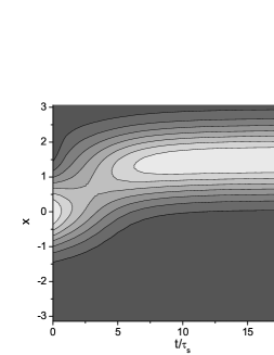
Figure 1: The neural response profile tracks the change of position of the external stimulus from $z_{0}=0$ to $1.5$ at $t=0$. Parameters: $a=0.5$, $\overline{k}=0.95$, $\overline{\beta}=0$, $\alpha=0.5$.

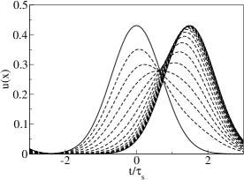
Figure 2: The profile of $u(x,t)$ at $t/\tau=0,1,2,\cdots,10$ during the tracking process in Fig. 1.

2.1 Dynamics of CANN without Dynamical Synapses

It is instructive to first consider the network dynamics when no dynamical synapses are included. This is done by setting $\beta=0$ in Eq. (2), so that $p(x,t)=1$ for all $t$. In this case, the network can support a continuous family of stationary states when the global inhibition is not too strong.

Specifically, the steady state solution to Eq. (1) is

$$\tilde{u}(x|z)=u_{0}\exp\left[-\frac{(x-z)^{2}}{4a^{2}}\right]\textrm{, }\quad\tilde{r}(x|z)=r_{0}\exp\left[-\frac{(x-z)^{2}}{2a^{2}}\right],$$ (3)

where $u_{0}=[1+(1-k/k_{c})^{1/2}]J_{0}/(4ak\sqrt{\pi})$, $r_{0}=[1+(1-k/k_{c})^{1/2}]/(2ak\rho\sqrt{2\pi})$ and $k_{c}=\rho J_{0}^{2}/(8a\sqrt{2\pi})$. These stationary states are translationally invariant among themselves and have the Gaussian shape with a free parameter $z$ representing the position of the Gaussian bumps. They exist for $0<k<k_{c}$, $k_{c}$ is thus the critical inhibition strength.

Fung et al [17] considered the perturbations of the Gaussian states. They found various distortion modes, each characterized by an eigenvalue representing its rate of evolution in time. A key property they found is that the translational mode has a zero eigenvalue, and all other distortion modes have negative eigenvalues for $k<k_{c}$. This implies that the Gaussian bumps are able to track changes in the position of the external stimuli by continuously shifting the position of the bumps, with other distortion modes affecting the tracking process only in the transients.

An example of the tracking process is shown in Figs. 1 and 2, when an external stimulus with a Gaussian profile is initially centered at $z=0$, pinning the center of a Gaussian neuronal response at the same position. At time $t=0$, the stimulus shifts its center from $z=0$ to $z=1.5$ abruptly. The bump moves towards the new stimulus position, and catches up with the stimulus change after a time duration. which is referred to as the reaction time.

3 Dynamics of CANN with Synaptic Depression

For clarity, we will first summarize the main results obtained on the network dynamics due to STD, and then present the theoretical analysis in Sec. 4.

3.1 The Phase Diagram

In the presence of STD, CANNs exhibit new interesting dynamical behaviors. Apart from the static bump state, the network also supports moving bump states. To construct a phase diagram mapping these behaviors, we first consider how the global inhibition $k$ and the synaptic depression $\beta$ scale with other parameters. In the steady state solution of Eq. (1), $u_{0}$ and $\rho J_{0}u_{0}^{2}$ should have the same dimension; so are $1-p(x,t)$ and $\tau_{d}\beta u_{0}$ in Eq. (2). Hence we introduce the dimensionless parameters $\overline{k}\equiv k/k_{c}$ and $\overline{\beta}\equiv\tau_{d}\beta/(\rho^{2}J_{0}^{2})$. The phase diagram obtained by numerical solutions to the network dynamics is shown in Fig. 3.

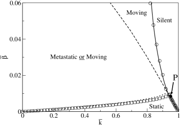
Figure 3: Phase diagram of the network states. Symbols: numerical solutions. Dashed line: Eq. (10). Dotted line: Eq. (13). Solid line: Gaussian approximation using $11^{\rm th}$ order perturbation of the STD coefficient. Point P: the working point for Figs. 4 and 7. Parameters: $\tau_{d}/\tau_{s}=50$, $a=0.5/6$, range of the network = $[-\pi,\pi)$.

We first note that the synaptic depression and the global inhibition plays the same role in reducing the amplitude of the bump states. This can be seen from the steady state solution of $u(x,t)$, which reads

$$u(x)=\int dx^{\prime}\frac{\rho J(x-x^{\prime})u(x^{\prime})^{2}}{1+k\rho\int dx^{\prime\prime}u(x^{\prime\prime})^{2}+\tau_{d}\beta u(x^{\prime})^{2}}.$$ (4)

The third term in the denominator of the integrand arises from STD, and plays the role of a local inhibition that is strongest where the neurons are most active. Hence we see that the silent state with $u(x,t)=0$ is the only stable state when either $\overline{k}$ or $\overline{\beta}$ is large.

When STD is weak, the network behaves similarly with CANNs without STD, that is, the static bump state is present up to $\overline{k}$ near 1. However, when $\overline{\beta}$ increases, a state with the bump spontaneously moving at a constant velocity comes into existence. Such moving states have been predicted in CANNs [12, 13], and can be associated with traveling wave behaviors widely observed in the neocortex [18]. At an intermediate range of $\overline{\beta}$, both the static and moving states coexist, and the final state of the network depends on the initial condition. When $\overline{\beta}$ increases further, only the moving state is present.

3.2 The Plateau Behavior

The network dynamics displays a very interesting behavior in the parameter regime when the static bump solution just loses its stability. In this regime, an initially activated network state decays very slowly to silence, in the time order of $\tau_{d}$. Hence, although the bump state eventually decays to the silent state, it goes through a plateau region of a slowly decaying amplitude, as shown in Fig. 4.

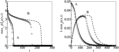
Figure 4: Magnitudes of rescaled neuronal input $\rho J_{0}u(x,t)$ and synaptic depression $1-p(x,t)$ at $(\overline{k},\overline{\beta})=(0.95,0.0085)$ (point P in Fig. 3) and for initial conditions of types A and B in Fig. 8. Symbols: numerical solutions. Lines: Gaussian approximation using Eqs. (8) and (9). Other parameters: $\tau_{d}/\tau_{s}=50$, $a=0.5$ and $x\in[-\pi,\pi)$.

3.3 Enhanced Tracking Performance

The responses of CANNs with STD to an abrupt change of stimulus are illustrated in Fig. 5. Compared with networks without STD, we find that the bump shifts to the new position faster. The extent of improvement in the presence of STD is quantified in Fig. 6. However, when $\overline{\beta}$ is too strong, the bump tends to overshoot the target before eventually approaching it.

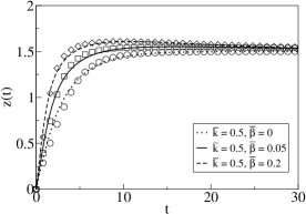
Figure 5: The response of CANNs with STD to an abruptly changed stimulus from $z_{0}=0$ to $z_{0}=1.5$ at $t=0$. Symbols: numerical solutions. Lines: Gaussian approximation using $11^{\rm th}$ order perturbation of the STD coefficent. Parameters: $\tau_{d}/\tau_{s}=50$, $\alpha=0.5$, $a=0.5$ and $x\in[-\pi,\pi)$.

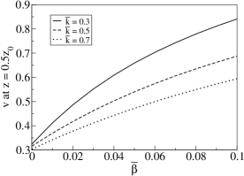
Figure 6: Tracking speed of the bump at $0.5z_{0}$, where $z_{0}$ is fixed to be 1.5

4 Analysis

Despite the apparently complex behaviors of CANNs with STD, we will show in this section that a Gaussian approximation can reproduce the behaviors and facilitate the interpretation of the results. Details are explained in Supplementary Information. We observe that the profile of the bump remains effectively Gaussian in the presence of synaptic depression. On the other hand, there is a considerable distortion of the profile of the synaptic depression, when STD is strong. Yet, to the lowest order approximation, let us approximate the profile of the synaptic depression to be a Gaussian as well, which is valid when STD is weak, as shown in Fig. 7(a). Hence, for $a\ll L$, we propose the following ansatz

$$u(x,t) = u_{0}(t)\exp\left[-\frac{(x-z)^{2}}{4a^{2}}\right],$$ (5)

$$p(x,t) = 1-p_{0}(t)\exp\left[-\frac{(x-z)^{2}}{2a^{2}}\right].$$ (6)

When these expressions are substituted into the dynamical equations (1) and (2), other functions $f(x)$ of $x$ appear. To maintain consistency with the Gaussian approximation, these functions will be approximated by their projections onto the Gaussian functions. In Eq. (1), we approximate

$$f(x)\approx\left[\int\frac{dx^{\prime}}{\sqrt{2\pi a^{2}}}f(x^{\prime})e^{-\frac{(x^{\prime}-z)^{2}}{4a^{2}}}\right]e^{-\frac{(x-z)^{2}}{4a^{2}}}.$$ (7)

Similarly, in Eq. (2), we approximate $f(x)$ by its projection onto $\exp\left[-(x-z)^{2}/(2a^{2})\right]$.

4.1 The Solution of the Static Bumps

Without loss of generality, we let $z=0$. Substituting Eq. (5) and (6) into Eqs. (1) and (2), and letting $\overline{u}(t)\equiv\rho J_{0}u_{0}(t)$, we get

$$\tau_{s}\frac{d\overline{u}(t)}{dt} = \frac{\overline{u}(t)^{2}}{\sqrt{2}(1+\overline{k}\overline{u}(t)^{2}/8)}\left[1-\sqrt{\frac{4}{7}}p_{0}(t)\right]-\overline{u}(t),$$ (8)

$$\tau_{d}\frac{dp_{0}(t)}{dt} = \frac{\overline{\beta}\overline{u}(t)^{2}}{1+\overline{k}\overline{u}(t)^{2}/8}\left[1-\sqrt{\frac{2}{3}}p_{0}(t)\right]-p_{0}(t).$$ (9)

By considering the steady state solution of $\overline{u}$ and $p_{0}$ and their stability against fluctuations of $\overline{u}$ and $p_{0}$, we find that stable solutions exist when

$$\overline{\beta}\leq\frac{p_{0}(1-\sqrt{4/7}p_{0})^{2}}{4(1-\sqrt{2/3}p_{0})}\left[1+\frac{\tau_{s}}{\tau_{d}(1-\sqrt{2/3}p_{0})}\right],$$ (10)

when $p_{0}$ is the steady state solution of Eqs. (1) and (2). The boundary of this region is shown as a dashed line in Fig. 3. Unfortunately, this line is not easily observed in numerical solutions since the static bump is unstable against fluctuations that are asymmetric with respect to its central position. Although the bump is stable against symmetric fluctuations, asymmetric fluctuations can displace its position and eventually convert it to a moving bump.

4.2 The Solution of the Moving Bumps

As shown in Fig. 7(b), the profile of a moving bump is characterized by a lag of the synaptic depression behind the moving bump. This is because neurons tend to be less active in locations of low values of $p(x,t)$, causing the bump to move away from locations of strong synaptic depression. In turn, the region of synaptic depression tends to follow the bump. However, if the time scale of synaptic depression is large, the recovery of the synaptic depressed region is slowed down, and cannot catch up with the bump motion. Thus, the bump starts moving spontaneously.

To incorporate asymmetry into the moving state, we propose the following ansatz:

$$u(x,t) = u_{0}(t)\exp\left[-\frac{(x-vt)^{2}}{4a^{2}}\right],$$ (11)

$$p(x,t) = 1-p_{0}(t)\exp\left[-\frac{(x-vt)^{2}}{2a^{2}}\right]+p_{1}(t)\exp\left[-\frac{(x-vt)^{2}}{2a^{2}}\right]\left(\frac{x-vt}{a}\right).$$ (12)

Projecting the terms in Eq. (1) to the basis functions $\exp\left[-(x-vt)^{2}/(4a^{2})\right]$ and $\exp\left[-(x-vt)^{2}/(4a^{2})\right](x-vt)/a$, and those in Eq. (2) to $\exp\left[-(x-vt)^{2}/(2a^{2})\right]$ and $\exp\left[-(x-vt)^{2}/(2a^{2})\right](x-vt)/a$, we obtain four equations for $\overline{u}$, $p_{0}$, $p_{1}$ and $v\tau_{s}/a$. Real solutions exist only if

$$\frac{\overline{\beta}\overline{u}^{2}}{1+\overline{k}\overline{u}^{2}/8}\geq A\left[\frac{\tau_{d}}{\tau_{s}}-B+\sqrt{\left(\frac{\tau_{d}}{\tau_{s}}-B\right)^{2}-C}\right]^{-1},$$ (13)

where $A=7\sqrt{7}/4$, $B=(7/4)[(5/2)\sqrt{7/6}-1]$, and $C=(343/36)(1-\sqrt{6/7})$. As shown in Fig. 3, the boundary of this region effectively coincides with the numerical solution of the line separating the static and moving phases.

Note that when $\tau_{d}/\tau_{s}$ increases, the static phase shrinks. This is because the recovery of the synaptic depressed region is slowed down, making it harder to catch up with changes in the bump motion.

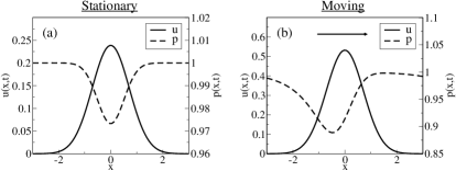
Figure 7: Neuronal input $u(x,t)$ and the STD coefficient $p(x,t)$ in (a) the static state at $(\overline{k},\overline{\beta})=(0.9,0.005)$, and (b) the moving state at $(\overline{k},\overline{\beta})=(0.5,0.015)$. Parameter: $\tau_{d}/\tau_{s}=50$.

An alternative approach that arrives at Eq. (13) is to consider the instability of the static bump, which is obtained by setting $v$ and $p_{1}$ to zero in Eqs. (11) and (12). Considering the instability of the static bump against the asymmetric fluctuations in $p_{1}$ and $vt$, we again arrive at Eq. (13). This shows that as soon as the moving bump comes into existence, the static bump becomes unstable. This also implies that in the entire region that the static and moving bumps coexist, the static bump is unstable to asymmetric fluctuations. It is stable (or more precisely, metastable) when it is static, but once it is pushed to one side, it will continue to move along that direction. We may call this behavior metastatic. As we shall see, this metastatic behavior is also the cause of the enhanced tracking performance.

4.3 The Plateau Behavior

To illustrate the plateau behavior, we select a point in the marginally unstable regime of the silent phase, that is, in the vicinity of the static phase. As shown in Fig. 8, the nullclines of $u$ and $p_{0}$ ($d\overline{u}/dt=0$ and $dp_{0}/dt=0$ respectively) do not have any intersections as they do in the static phase where the bump state exists. Yet, they are still close enough to create a region with very slow dynamics near the apex of the $u$-nullcline at $(\overline{u},p_{0})=[(8/\overline{k})^{1/2},\sqrt{7/4}(1-\sqrt{\overline{k}})]$. Then, in Fig. 8, we plot the trajectories of the dynamics starting from different initial conditions. For verification, we also solve the full equations (1) and (2), and plot a flow diagram with the axes being $\max_{x}u(x,t)$ and $1-\min_{x}p(x,t)$. The resultant flow diagram has a satisfactory agreement with Fig. 8.

The most interesting family of trajectories is represented by B and C in Fig. 8. Due to the much faster dynamics of $\overline{u}$, trajectories starting from a wide range of initial conditions converge rapidly, in a time of the order $\tau_{s}$, to a common trajectory in the close neighborhood of the $\overline{u}$-nullcline. Along this common trajectory, $\overline{u}$ is effectively the steady state solution of Eq. (8) at the instantaneous value of $p_{0}(t)$, which evolves with the much longer time scale of $\tau_{d}$. This gives rise to the plateau region of $\overline{u}$ which can survive for a duration of the order $\tau_{d}$. The plateau ends after the trajectory has passed the slow region near the apex of the $\overline{u}$-nullcline. This dynamics is in clear contrast with trajectory D, in which the bump height decays to zero in a time of the order $\tau_{s}$.

Trajectory A represents another family of trajectories having rather similar behaviors, although the lifetimes of their plateaus are not so long. These trajectories start from more depleted initial conditions, and hence do not have chances to get close to the $\overline{u}$-nullcline. Nevertheless, they converge rapidly, in a time of order $\tau_{s}$, to the band $\overline{u}\approx(8/\overline{k})^{1/2}$, where the dynamics of $\overline{u}$ is slow. The trajectories then rely mainly on the dynamics of $p_{0}$ to carry them out of this slow region, and hence plateaus of lifetimes of the order $\tau_{d}$ are created.

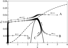
Figure 8: Trajectories of network dynamics starting from various initial conditions at $(\overline{k},\overline{\beta})$ = (0.95, 0.0085) (point P in Fig. 3). Solid line: $\overline{u}$-nullcline. Dashed line: $p_{0}$-nullcline. Symbols are data points spaced at time intervals of $2\tau_{s}$.

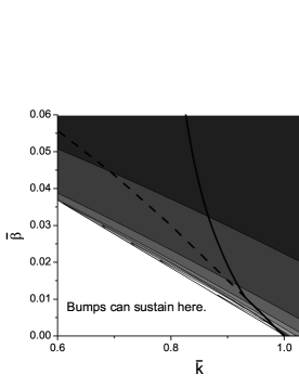
Figure 9: Contours of plateau lifetimes in the space of $\overline{k}$ and $\overline{\beta}$. The lines are the two topmost phase boundaries in Fig. 3. In the initial condition, $\alpha=0.5$.

Following similar arguments, the plateau behavior also exists in the stable region of the static states. This happens when the initial condition of the network lies outside the basin of attraction of the static states, but it is still in the vicinity of the basin boundary.

When one goes deeper into the silent phase, the region of slow dynamics between the $\overline{u}$- and $p_{0}$-nullclines broadens. Hence plateau lifetimes are longest near the phase boundary between the bump and silent states, and become shorter when one goes deeper into the silent phase. This is confirmed by the contours of plateau lifetimes in the phase diagram shown in Fig. 9 obtained by numerical solution. The initial condition is uniformly set by introducing an external stimulus $I^{\rm ext}(x|z_{0})=\alpha u_{0}\exp[-x^{2}/(4a^{2})]$ to the right hand side of Eq. (1), where $\alpha$ is the stimulus strength. After the network has reached a steady state, the stimulus is removed at $t=0$, leaving the network to relax.

4.4 The Tracking Behavior

To study the tracking behavior, we add the external stimulus $I^{\textrm{ext }}(x|z_{0})=\alpha u_{0}\exp\left[-(x-z_{0})^{2}/(4a^{2})\right]$ to the right hand side of Eq. (11), where $z_{0}$ is the position of the stimulus abruptly changed at $t=0$. With this additional term, we solve the modified version of Eqs. (11) and (12), and the solution reproduces the qualitative features due to the presence of synaptic depression, namely, the faster response at weak $\overline{\beta}$, and the overshooting at stronger $\overline{\beta}$. As remarked previously, this is due to the metastatic behavior of the bumps, which enhances their reaction to move from the static state when a small push is exerted.

However, when describing the overshooting of the tracking process, the quantitative agreement between the numerical solution and the ansatz in Eqs. (11) and (12) is not satisfactory. We have made improvement by developing a higher order perturbation analysis using basis functions of the quantum harmonic oscillator [17]. As shown in Fig. 5, the quantitative agreement is much more satisfactory.

5 Conclusions and Discussions

In this work, we have investigated the impact of STD on the dynamics of a CANN, and found that the network can support both static and moving bumps. Static bumps exist only when the synaptic depression is sufficiently weak. A consequence of synaptic depression is that it places static bumps in the metastatic state, so that its response to changing stimuli is speeded up, enhancing its tracking performance. We conjecture that moving bump states may be associated with traveling wave behaviors widely observed in the neurocortex.

A finding in our work with possibly very important biological implications is that STD endows the network with slow-decaying behaviors. When the network is initially stimulated to an active state by an external input, it will decay to silence very slowly after the input is removed. The duration of the plateau is of the time scale of STD rather than neural signaling, and it provides a way for the network to hold the stimulus information for up to hundreds of milliseconds, if the network operates in the parameter regime that the bumps are marginally unstable. This property is, on the other hand, extremely difficult to be implemented in attractor networks without STD. In a CANN without STD, an active state of the network decays to silence exponentially fast or persists forever, depending on the initial activity level of the network. Indeed, how to shut off the activity of a CANN has been a challenging issue that received wide attention in theoretical neuroscience, with solutions suggesting that a strong external input either in the form of inhibition or excitation must be applied (see, e.g., [19]). Here, we show that STD provides a mechanism for closing down network activities naturally and in the desirable duration.

We have also analyzed the dynamics of CANNs with STD using a Gaussian approximation of the bump. It describes the phase diagram of the static and moving phases, the plateau behavior, and provides insights on the metastatic nature of the bumps and its relation with the enhanced tracking performance. In most cases, approximating $1-p(x,t)$ by a Gaussian profile is already sufficient to produce qualitatively satisfactory results. However, higher order perturbation analysis is required to yield more accurate descriptions of results such as the overshooting in the tracking process (Fig. 5).

Besides STD, there are other forms of STP that may be relevant to realizing short-term memory. Mongillo et al. [20] have recently proposed a very interesting idea for achieving working memory in the prefrontal cortex by utilizing the effect of short-term facilitation (STF). Compared with STD, STF has the opposite effect in modifying the neuronal connection weights. The underlying biophysics of STF is the increased level of residual calcium due to neural firing, which increases the releasing probability of neural transmitters. Mongillo et al. [20] showed that STF provides a way for the network to encode the information of external inputs in the facilitated connection weights, and it has the advantage of not having to recruit persistent neural firing and hence is economically efficient. This STF-based memory mechanism is, however, not necessarily contradictory to the STD-based one we propose here. They may be present in different cortical areas for different computational purposes. STD and STF have been observed to have different effects in different cortical areas. One location is the sensory cortex where CANN models are often applicable. Here, the effects of STD tends to be stronger than that of STF. Different from the STF-based mechanism, our work suggests that the STD-based one exhibits the prolonged neural firing, which has been observed in some cortical areas. In terms of information transmission, prolonged neural firing is preferable in the early information pathways, so that the stimulus information can be conveyed to higher cortical areas through neuronal interactions. Hence, it seems that the brain may use a strategy of weighting the effects of STD and STF differentially for carrying out different computational tasks. It is our goal in future work to explore the joint impact of STD and STF on the dynamics of neuronal networks.

This work is partially supported by the Research Grants Council of Hong Kong (grant nos. HKUST 603607 and 604008).

References

- [1] H. Markram, Y. Wang and M. Tsodyks, Proc. Natl. Acad. Sci. U.S.A., 95, 5323 (1998).
- [2] M. Tsodyks and H. Markram, Proc. Natl. Acad. Sci. U.S.A., 94, 719-723 (1997).
- [3] L. F. Abbott, J. A. Varela, K. Sen and S. B. Nelson, Science, 275, 220-224 (1997).
- [4] M. Tsodyks, A. Uziel and H. Markram, J. Neurosci., 20, 1-5 (2000).
- [5] A. Loebel and M. Tsodyks, J. Comput. Neurosci., 13, 111-124 (2002).
- [6] J.-P. Pfister, P. Dayan, and M. Lengyel, Advances in Neural Information Processing Systems 22, Y. Bengio, D. Schuurmans, J. Lafferty, C. K. I. Williams, and A. Culotta (eds.), 1464 (2009).
- [7] S. Amari, Biological Cybernetics, 27, 77-87 (1977).
- [8] R. Ben-Yishai, R. Lev Bar-Or and H. Sompolinsky, Proc. Natl. Acad. Sci. U.S.A., 92, 3844-3848 (1995).
- [9] K.-C. Zhang, J. Neurosci., 16, 2112-2126 (1996).
- [10] A. Samsonovich, and B. L. McNaughton, J. Neurosci., 7, 5900-5920 (1997).
- [11] S. Deneve, P. E. Latham and A. Pouget, Nature Neuroscience, 2, 740-745 (1999).
- [12] L. C. York and M. C. W. van Rossum, J. Comput. Neurosci. 27, 607-620 (2009)
- [13] Z. P. Kilpatrick and P. C. Bressloff, Physica D 239, 547-560 (2010)
- [14] J. Hao, X. Wang, Y. Dan, M. Poo and X. Zhang, Proc. Natl. Acad. Sci. U.S.A., 106, 21906-21911 (2009).
- [15] M. V. Tsodyks, K. Pawelzik and H. Markram, Neural Comput. 10, 821-835 (1998).
- [16] R. S. Zucker and W. G. Regehr, Annu. Rev. Physiol. 64, 355-405 (2002).
- [17] C. C. A. Fung, K. Y. M. Wong and S. Wu, Neural Comput. 22, 752-792 (2010)
- [18] J. Wu, X. Huang and C. Zhang, The Neuroscientist, 14, 487-502 (2008).
- [19] B. S. Gutkin, C. R. Laing, C. L. Colby, C. C. Chow and B. G. Ermentrout, J. Comput. Neurosci., 11, 121-134 (2001).
- [20] G. Mongillo, O. Barak and M. Tsodyks, Science, 319, 1543-1546 (2008).