Edge and bulk components of lowest-Landau-level orbitals, correlated fractional quantum Hall effect incompressible states, and insulating behavior in finite graphene samples

Abstract

Many-body calculations of the total energy of interacting Dirac electrons in finite graphene samples exhibit joint occurrence of cusps at angular momenta corresponding to fractional fillings characteristic of formation of incompressible (gapped) correlated states ($\nu=1/3$ in particular) and opening of an insulating energy gap (that increases with the magnetic field) at the Dirac point, in correspondence with experiments. Single-particle basis functions obeying the zigzag boundary condition at the sample edge are employed in exact diagonalization of the interelectron Coulomb interaction, showing, at all sizes, mixed equal-weight bulk and edge components. The consequent depletion of the bulk electron density attenuates the fractional-quantum-Hall-effect excitation energies and the edge charge accumulation results in a gap in the many-body spectrum.

I Introduction

The isolation of graphene sheets geim04 was soon followed by experiments geim05 ; kim05 on the anomalous integer quantum Hall effect (IQHE), demonstrating the formation of Landau levels, described with non-interacting electron theory. Subsequently, theoretical explorations jain06 ; chak06 appeared pertaining to the fractional quantum Hall effect (FQHE) in graphene, which, in contrast to the IQHE, is known to be the manifestation of collective correlated interacting electrons phenomena. For Dirac electrons in the lowest ($n$ = 0) Landau level (LLL), it was found jain06 ; chak06 (in a spherical geometry) that the behavior of the incompressible states in boundless graphene models emulates that of the well-known FQHE in the semiconductor 2D electron gas. laug83 ; yann07 ; jainbook Recent experiments, andr09 ; kim09 employing small (1 $\mu$m) suspended single-sheet samples have shown that the appearance of the FQHE in graphene is accompanied by the emergence of an insulating phase. The physics that underlies this joint occurrence, coupled with the systematic theoretical overestimation jain06 ; chak06 of the measured FQHE excitation energies, remains unresolved; similar findings in recent experiments on bilayer graphene bao10 further highlight these open issues.

In this paper, we show, using exact diagonalization yann07 (EXD) (in the quantum Hall regime) of the many-body hamiltonian for interacting Dirac electrons occupying the LLL of finite planar graphene samples, that the incompressible correlated electron physics is modified [using zigzag boundary conditions geim09 (ZBC)] in two main ways: (i) the FQHE excitation energies are significantly attenuated due to depletion of the density of the bulk component of the Dirac electrons spinor, and (ii) the concurrent accumulation of charge at the sample edge underlies the opening of a gap in the many-electron spectrum (increasing with the magnetic field, as observed experimentally), relating to the aforementioned insulating phase.

Underlying the above many-body behavior is the existence of LLL single-particle states of mixed character, exhibiting bulk- [Darwin-Fock-type yann07 (DF)] and edge-type components of equal weights note56 (independent of sample size), each residing on a different graphene sublattice. With interelectron repulsion, the bulk component exhibits FQHE characteristics (with excitation energy gaps reduced by a factor of four compared to boundless graphene). The edge component is associated with formation of a single-ring rotating Wigner molecule yann07 (RWM). The size-independent influence of the graphene edge on the many-body properties ushers a new paradigm, contrasting the commonly accepted expectation that materials bulk properties are unaffected by the detailed configuration or conditions at the surface. peierls This unique behavior derives from the two-sublattice topology of the graphene net modeled here by the continuous Dirac-Weyl (DW) equation. geim09

An important element in our approach is formulation of the solutions of the Dirac-Weyl equation (with the zigzag boundary conditions) using the Kummer confluent hypergeometric function. abrabook This formulation provides systematic analytical insights into the nature of the DW single-particle states (bulk and edge), as well as it permits efficient and accurate numerical evaluations (with the help of algebraic computer languages mathbook ).

In Sec. II we describe the confluent-hypergeometric-function formulation of the solutions of the DW equation and construct the LLL DW spinor in terms of equal-weight bulk and edge components. Details of the solutions of the DW equation in polar coordinates are given in Appendix A.

A brief description of the exact-diagonalization many-body method, and the contributions of the bulk and edge spinor components to the Coulomb interaction matrix elements are given in Sec. III.

In Sec. IV we display results for the ground-state and excited spectra, and their relation to the $\nu=1/3$ FQHE incompressible state and to the insulating behavior at $\nu=0$.

A summary is presented in Sec. V.

Finally, in Appendix B we distinguish the mixed bulk-edge Dirac spinor states (forming the quasidegenerate LLL manifold in finite graphene samples with ZBC), where one of the spinor components is located in the bulk of the sample and the other localized at the edge, from the “double-edge” states where both components of the spinor represent edge states. In the “double-edge” case, one component corresponds to a bulk orbital which transforms (when the orbital’s centroid falls near the graphene sample boundary) into an edge state familiar from the theoryhalp82 of the nonrelativistic integer QHE. The other component of the “double-edge” spinor, as well as the edge orbital of the aforementioned mixed bulk-edge one, corresponds to an edge state unique to the two sublattice topology of graphene. We discuss and illustrate the natural way in which the above classification of Dirac-electron edge states arises within the framework of the Kummer function formalism for the solution of the DW equation described in Sec. II and Appendix A.

II The single-particle lowest-Landau-level manifold with zigzag boundary conditions

We first discuss the solution of the Dirac-Weyl equation in polar coordinates under the imposition of the zigzag boundary condition. We model the low-energy noninteracting graphene electrons (around a given $K$ point) via the continuous DW equation. geim09 Circular symmetry leads to conservation of the total pseudospin geim09 $\hat{\jmath}=\hat{l}+\hat{\sigma}_{z}$, where $\hat{l}$ is the angular momentum of a Dirac electron. As a result, we seek solutions for the two components $\psi^{A}({\bf r})$ and $\psi^{B}({\bf r})$ (associated with the two graphene sublattices $A$ and $B$) of the single-particle electron orbital (a spinor) that have the following general form in polar coordinates:

$$\psi_{l}({\bf r})=\left(\begin{array}[]{c}\psi^{A}({\bf r})\\ \psi^{B}({\bf r})\end{array}\right)=\left(\begin{array}[]{c}e^{il\phi}\chi^{A}(r)\\ ie^{i(l+1)\phi}\chi^{B}(r)\end{array}\right).$$ (1)

The angular momentum takes integer values; for simplicity in Eq. (1) and in the following, the subscript $l$ is omitted in the sublattice components $\psi^{A}$, $\psi^{B}$ and $\chi^{A}$, $\chi^{B}$.

With Eq. (1) and a constant magnetic field $B$ (symmetric gauge), the DW equation reduces (for the $K$ valley) to

$$\frac{d}{dx}\chi^{B}+\frac{1}{x}\left(l+1+\frac{x^{2}}{2}\right)\chi^{B} = \varepsilon\chi^{A}$$

$$\frac{d}{dx}\chi^{A}-\frac{1}{x}\left(l+\frac{x^{2}}{2}\right)\chi^{A} = -\varepsilon\chi^{B},$$ (2)

where the reduced radial coordinate $x=r/l_{B}$ with $l_{B}=\sqrt{\hbar c/(eB)}$ the magnetic length. The reduced single-particle eigenenergies $\varepsilon=E/(\hbar v_{F}/l_{B})$, with $v_{F}$ the Fermi velocity. Since the properties of the solutions of the DW equation with a magnetic field using the ZBC are not widely known, we outline pertinent details on this subject in the following (see also Appendices A and B).

For a finite circular graphene sample of radius $R$, we seek solutions of Eq. (2) for $\varepsilon\neq 0$ with $l\leq-1$ (corresponding to $j<-1/2$) that are regular at the origin ($x=0$). The general form of solution is

$$\chi^{A}(x)=-{\cal C}\frac{\varepsilon}{2|l|}e^{-x^{2}/4}x^{|l|}M\left(1-\frac{\varepsilon^{2}}{2},|l|+1,\frac{x^{2}}{2}\right),$$

$$\chi^{B}(x)={\cal C}e^{-x^{2}/4}x^{|l|-1}M\left(-\frac{\varepsilon^{2}}{2},|l|,\frac{x^{2}}{2}\right),$$ (3)

where $M(a,b,z)$ is Kummer’s confluent hypergeometric function abrabook and ${\cal C}$ is a normalization constant.

The ZBC requires that one sublattice component vanishes at the physical edge situated at the finite radius $R$ of the graphene sample. Therefore at least one of the Kummer functions in Eq. (3) must exhibit zeros (nodes) for $x>0$. The search for such zeros is greatly facilitated with the use of the following theorem: gatt08 For the Kummer function $M(a,b,z)$ ($z$ being real), it is known that, if $b>0$ [which is the case for both Kummer functions in Eq. (3)], there are no zeros of $M(a,b,z)$ for $z>0$ if $a\geq 0$, and there are precisely $-\lfloor a\rfloor$ zeros if $a<0$; the floor function is defined as: $\lfloor a\rfloor=n$ if and only if $n\leq a<n+1$, where $n$ is any positive or negative integer (including zero).

The $\chi^{B}$ LLL component does exhibit precisely one zero, enabling a transcendental equation (for a given $x_{R}$) for the single-particle energies $\varepsilon$

$$\chi^{B}(\varepsilon,l,x_{R})=0,\;\;\;\text{or}\;\;\;M\left(-\frac{\varepsilon^{2}}{2},|l|,\frac{x_{R}^{2}}{2}\right)=0.$$ (4)

The solutions to Eq. (4) (for a range of $x_{R}>>1$, i.e., high magnetic fields, and for any $l\leq-1$) give states (which compose the LLL manifold) with near vanishing energies $0<\varepsilon/\sqrt{2}<<1$. Consequently, within the graphene sample, when $R/l_{B}>>1$, $\chi^{B}$ can be approximated by a bulk-type DF orbital, i.e.,

$$|b\rangle={\cal C}e^{-x^{2}/4}x^{|l|-1},$$ (5)

with ${\cal C}=1/\sqrt{2^{|l|-1}\Gamma(|l|)}$ normalizing $|b\rangle$ to unity in $[0,x_{R}]$.

From the theorem discussed above, it follows that the $\chi^{A}$ LLL component cannot have any zeros, and thus for $x_{R}=R/l_{B}>>1$ it will develop into an edge state

$$|e\rangle=-|\widetilde{\cal C}|e^{x^{2}/4}x^{|l|},$$ (6)

due to the asymptotic behavior abrabook ; note32

$$M(1-\varepsilon^{2}/2,|l|+1,x^{2}/2)\sim\exp(x^{2}/2)x_{R}^{-2|l|}$$ (7)

for $x\sim x_{R}$. The normalization constant $\widetilde{\cal C}$ conforms to the requirement that $\chi^{A}$ and $\chi^{B}$ [see Eq. (1)] should have equal weights for the $\varepsilon$’s obtained via solution of Eq. (4); $\widetilde{\cal C}$ is determined from $\widetilde{\cal C}^{2}\int_{0}^{x_{R}}e^{x^{2}/2}x^{2|l|+1}dx=1$.

Finally, for $R/l_{B}>>1$, the following simplified expression for the LLL spinor can be written:

$$\psi_{l}({\bf r})=\frac{1}{\sqrt{2}}\left(\begin{array}[]{c}e^{il\phi}|e\rangle/\sqrt{2\pi}\\ ie^{i(l+1)\phi}|b\rangle/\sqrt{2\pi}\end{array}\right),$$ (8)

where $|b\rangle$ and $|e\rangle$ are each normalized to unity in $[0,x_{R}]$. A numerical graphical illustration showing that the general expression for the spinor components in Eq. (3) can be well approximated by Eq. (8) is given in Appendix B.

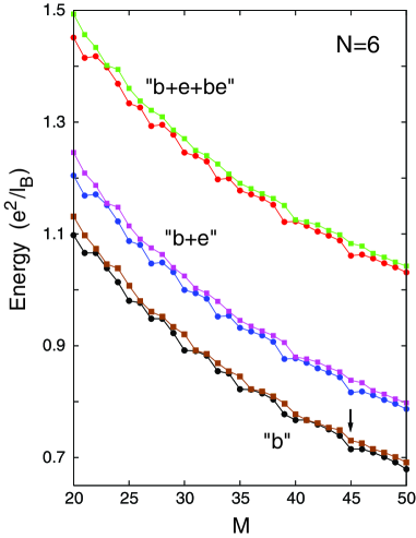
Figure 1: EXD energies for $N=6$ Dirac electrons. Energies for the lowest (yrast, solid dots) and first-excited states (solid squares) are plotted as a function of the total angular momentum $M=\sum_{i=1}^{N}m_{i}$ ($m_{i}\equiv|l_{i}|$). “b”, “e”, and “be” denote, respectively, the bulk, edge, and cross bulk-edge contributions to the total energies. The “b” contribution reflects a 50% depletion of the bulk component due to the form of the Dirac-electron spinor in Eq. (8). The arrow in the “b” curve points to the $\nu=1/3$ ($M=45$) excitation energy gap (the difference between first-excited and yrast energies). The radius of the sample was taken as $R=30l_{B}$. $\kappa=1$ for suspended graphene.

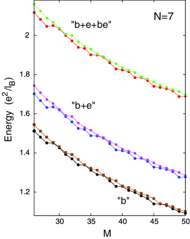
Figure 2: EXD energies for $N=7$ Dirac electrons. Energies for the lowest (yrast, solid dots) and first-excited states (solid squares) are plotted as a function of the total angular momentum $M=\sum_{i=1}^{N}m_{i}$ ($m_{i}\equiv|l_{i}|$). “b”, “e”, and “be” denote, respectively, the bulk, edge, and cross bulk-edge contributions to the total energies. The “b” contribution reflects a 50% depletion of the bulk component due to the form of the Dirac-electron spinor in Eq. (8). The radius of the sample was taken as $R=25l_{B}$. $\kappa=1$ for suspended graphene.

III Exact diagonalization of the many-body problem

In the EXD method, yann07 the many-body wave function is given as a linear superposition

$$\Phi^{\text{EXD}}_{M}[{\bf r}_{1},\ldots,{\bf r}_{N}] =$$ (9)

$$\sum_{m_{1}<\ldots<m_{N}}^{m_{1}+\ldots+m_{N}=M}{\cal V}(m_{1},\ldots,m_{N})\Psi^{m_{1},\ldots,m_{N}}[{\bf r}_{1},\ldots,{\bf r}_{N}],$$

where the Slater determinants $\Psi^{m_{1},\ldots,m_{N}}$ are constructed out of the quasidegenerate ($\varepsilon\sim 0$) LLL spinor orbitals $\psi_{l}({\bf r})$ [see Eq. (8)], where we define $m=|l|$; $l\leq-1$. We omit the Coulomb coupling between valleys, and also consider fully spin-polarized electrons.

The eigenvectors ${\cal V}$’s in Eq. (9) and corresponding many-body energies $E^{\text{EXD}}$ are calculated through a direct matrix diagonalization of the many-body hamiltonian

$$H=\sum_{i<j}V_{C}(i,j),$$ (10)

where $V_{C}(i,j)=e^{2}/(\kappa|{\bf r}_{i}-{\bf r}_{j}|)$ is the two-body Coulomb interaction, within the Hilbert space of Slater determinants yann07 $\Psi^{m_{1},\ldots,m_{N}}$. Being constant (here $\approx 0$), the kinetic energy terms in the many-body hamiltonian Eq. (10) have been neglected. yann07 ; jainbook

The EXD computations require an accurate evaluation of the two-body Coulomb matrix elements

$$\int\int d{\bf r}_{1}d{\bf r}_{2}\psi^{*}_{m_{1}}({\bf r}_{1})\psi^{*}_{m_{2}}({\bf r}_{2})V_{C}(1,2)\psi_{m_{3}}({\bf r}_{1})\psi_{m_{4}}({\bf r}_{2}),$$ (11)

which expand to a sum of four similar integrals. Denoting $|\tilde{b}_{m}\rangle=ie^{i(l+1)\phi}|b\rangle/\sqrt{2\pi}$ and $|\tilde{e}_{m}\rangle=e^{il\phi}|e\rangle/\sqrt{2\pi}$, this expansion is written as

$$\frac{1}{4}(\langle\tilde{b}_{1}\tilde{b}_{2}|\tilde{b}_{3}\tilde{b}_{4}\rangle+\langle\tilde{e}_{1}\tilde{e}_{2}|\tilde{e}_{3}\tilde{e}_{4}\rangle+\langle\tilde{b}_{1}\tilde{e}_{2}|\tilde{b}_{3}\tilde{e}_{4}\rangle+\langle\tilde{e}_{1}\tilde{b}_{2}|\tilde{e}_{3}\tilde{b}_{4}\rangle).$$ (12)

Note that, due to the equal weights of the bulk-like and edge-like components, a prefactor of 1/4 appears in front of each term in Eq. (12); the consequences of this prefactor are discussed in Sec. IV.1.

IV Results

IV.1 Energetics

In Figs. 1 and 2, we display total EXD energies for the yrast (i.e., the lowest in energy) and first-excited states of spin-polarized electrons in a graphene finite sample with $N=6$ and $N=7$ Dirac electrons as a function of the total angular momentum $M$ (which is conserved in the EXD calculation). Moreover, the displayed energies correspond to: (i) only the bulk-type terms (“b”), (ii) combined bulk-type and edge-type terms (“b$+$e”), and (iii) with the inclusion of cross bulk-edge terms (“b$+$e$+$be”) in the two-body Coulomb matrix elements [see Eq. (12)]. Each of the terms (“b”, “e”, and “be”) is reduced by a factor of 1/4 as discussed above. For all cases, we note the appearance of cusp states (states with enhanced stability and larger excitation gaps relative to their immediate neighborhood yann07 ; jainbook ; laug83.2 ) at the magic angular momenta

$$M_{m}=M_{0}+kN\mbox{~{}~{}or~{}~{}}M_{m}=M_{0}+k(N-1),$$ (13)

where $M_{0}=N(N-1)/2$, $k=0,1,2,3,\ldots$, and $N$ is the number of electrons. For the bulk component, the cusp states are interpreted jainbook ; laug83.2 as a signature of the formation of correlated incompressible states that may exhibit certain correlated liquid characteristics and underlie the FQHE physics in the thermodynamic limit. In particular, the magic angular momenta are associated jainbook ; laug83.2 with fractional fillings $\nu=M_{0}/M_{m}$. Note that the angular momenta of the Laughlin FQHE function laug83 correspond to Eq. (13) with $k=(N-1)p$ for the first case and $k=Np$ for the second case, with the associated fractions given by $\nu=1/(2p+1)$ ($p$ being a positive integer).

The EXD energies displayed in Fig. 1 and 2 [and additional calculated results for other sizes $N=3-5$ and $8$ (not shown)] reveal three prominent trends:

(I) The “b$+$e” energies are always higher than those calculated only with the bulk-type component (denoted as “b”). More importantly (as checked for various sample sizes, e.g., $R/l_{B}=15,25$ and 30), the difference between the “b$+$e” (i.e., including the edge contribution) and “b” EXD energies (for any $N$) approaches asymptotically for $M\rightarrow\infty$ the value $\Delta E_{1}(N)/4$; $\Delta E_{1}(N)$ is the electrostatic energy of $N$ point charges localized on the perimeter at the vertices of a regular polygon, i.e.,

$$\Delta E_{1}(N)=\frac{NS_{N}}{4x_{R}}\frac{e^{2}}{\kappa l_{B}},$$ (14)

with $S_{N}=\sum_{j=2}^{N}\big{(}\sin[(j-1)\pi/N]\big{)}^{-1}$. The factor 1/4 is due to the half weight of the electrons accumulating on the physical edge [recall the spinor in Eq. (8)]. The result in Eq. (14) (deduced from analysis of the EXD computed energies, see, e.g., Figs. 1 and 2) suggests that a single-ring Wigner molecule is formed at the edge; this is in agreement with the CPD analysis in Sec. IV.2.

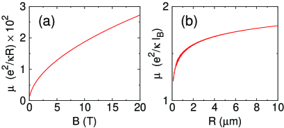
Figure 3: Variation of the insulating gap $\mu$. (a) As a function of $B$ when $R=1$ $\mu$m. (b) As a function of $R$ when $B=8$ T. Note the $\mu\propto B^{0.54}$ increase shown in (a) and the effective saturation for large $R$ exhibited in (b). $\alpha=2$.

(II) The “b$+$e$+$be” energies are always higher than the “b$+$e” ones. Moreover, the difference between the “b$+$e$+$be” and “b$+$e” EXD energies (for any $N$) approach asymptotically for $M\rightarrow\infty$ the value $\Delta E_{2}(N)/4$, where $\Delta E_{2}(N)$ is the electrostatic energy due to the repulsion between a point charge of strength $Ne$ located at the center and $Ne$ charges distributed at the perimeter of the sample,

$$\Delta E_{2}(N)=\frac{N(N-1)}{x_{R}}\frac{e^{2}}{\kappa l_{B}}.$$ (15)

The factor 1/4 is again due to half of the electrons being accumulated on the physical edge, while the other half being located in the bulk component; the factor $N-1$ accounts for the self-interaction correction.

It is apparent that the EXD density of states associated with the “b$+$e$+$be” LLL spectrum will show (for a given $N$) the opening of an interaction-induced energy gap

$$\Delta E(N)=\Delta E_{1}(N)/4+\Delta E_{2}(N)/4$$ (16)

compared to that associated with the bulk-only (“b”) spectrum. The emergence of this edge-induced, electrostatic energy gap is related to (see below) the experimentally observed andr09 ; kim09 insulating behavior at the charge neutrality point ($\nu=0$).

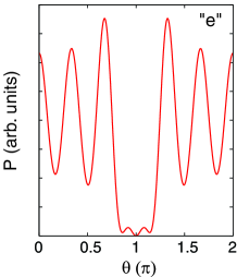
Figure 4: CPD for the edge component portraying the formation of a single-ring RWM. An illustrative yrast cusp state (with $N=6$ and $M=39$) in a graphene sample of radius $R/l_{B}=30$ is considered. The azimuthal CPD at the physical edge of the sample is plotted, i.e., ${\cal P}({\bf r},{\bf r}_{0})$ as a function of ${\bf r}=30(\cos\theta,\sin\theta)$. The fixed point is located at ${\bf r}_{0}=30(\cos\pi,\sin\pi)$. Note the five maxima corresponding to the remaining five electrons, with the sixth one taken at ${\bf r}_{0}$. ${\bf r}$ and ${\bf r}_{0}$ are in units of $l_{B}$.

(III) Due to the fact that both the “e” and “e$+$be” contributions (expressed in units of $e^{2}/\kappa l_{B}$) decrease as a function of $R/l_{B}$ [see points (I) and (II) above, and the factor $1/x_{R}=l_{B}/R$ in Eqs. (14) and (15)], it follows that in the thermodynamic limit the excitation gaps (which determine the strength of the FQHE) will approach those of the “b” contribution alone (which is independent of $R/l_{B}$). As a result, the FQHE excitation energy gaps for a graphene sample with zigzag edges (and in particular for $\nu=1/3$) are 1/4 [see the prefactor of the bulk-only contribution in Eq. (12)] of those calculated jain06 ; chak06 using boundless-graphene modeling. For boundless graphene, available in the literature EXD calculations in a spherical geometry reported two values for the FQHE energy gap: the first value andr09 ; chak06 is $\sim$ 0.1 $e^{2}/\kappa l_{B}$ for polarized electrons, while the second value jain06 is 0.042 $e^{2}/\kappa l_{B}$ when pseudoskyrmion effects are considered. note12 From our disk-geometry EXD calculations, we find (in units of $e^{2}/\kappa l_{B}$, and including the above 1/4 factor) an excitation energy gap for the “b” component of 0.0153 ($N=6$, $M_{1/3}=45$), 0.0160 ($N=7$, $M_{1/3}=63$), 0.0145 ($N=8$, $M_{1/3}=84$), 0.0150 ($N=9$, $M_{1/3}=108$), 0.0149 ($N=10$, $M_{1/3}=135$), and 0.0147 ($N=11$, $M_{1/3}=165$) ($M_{1/3}$ gives the magic angular momenta corresponding to $\nu=1/3$). These values extrapolate to an excitation energy gap of $0.0137$ $e^{2}/\kappa l_{B}$ for $N\rightarrow\infty$ (with a standard error of $\pm 0.0009$). Our result is in good agreement with the experimentally measured andr09 ; kim09 value (0.008 $e^{2}/\kappa l_{B}$), with a possible added effect of residual disorder.

To estimate the magnitude of the experimentally observable insulating gap, $\mu(\nu=0)=\Delta E(N_{\text{max}}+1)-\Delta E(N_{\text{max}})$ [recall Eq. (16)], one needs to consider the maximum number, $N_{\text{max}}$, of RWM electrons on the edge of the graphene disk [see point (I) above]. A rough estimate is given by $N_{\text{max}}\sim 2\pi R/(2\alpha l_{B})$, where $R$ is the radius of the graphene sample and $\alpha$ is a fitting parameter. The variation of $\mu(\nu=0)$ with $B$ shown in Fig. 3(a) (calculated for $R=1$ $\mu$m) is found to behave as $B^{\gamma}$, $\gamma\approx 0.54$; the increase of the gap with $B$ is consistent with recent experiments on suspended graphene. andr09 ; kim09 The evolution of the insulating gap with the size of the system is found to essentially saturate for large $R$ [see Fig. 3(b) calculated for $B=8$ T].

IV.2 Conditional probability distributions for the edge component

The calculated electron density is azimuthally uniform due to the conservation of the total angular momentum $M$ in the many-body EXD calculations. The spatial arrangement of the edge-type component of the $N$ correlated electrons can be revealed in the intrinsic frame of reference via the two-body correlation function yann07 ${\cal P}({\bf r},{\bf r}_{0})$, referred to as a conditional probability distribution (CPD). The CPD is defined as

$${\cal P}({\bf r},{\bf r}_{0})\propto\langle\Phi^{\text{EXD}}_{M}|\sum_{i\neq j}\delta({\bf r}_{i}-{\bf r})\delta({\bf r}_{j}-{\bf r}_{0})|\Phi^{\text{EXD}}_{M}\rangle.$$ (17)

The CPDs are giving the probability of finding one electron at position ${\bf r}$ assuming that another one is fixed at the point ${\bf r}_{0}$. The CPD for the edge (“e”) component of the yrast cusp state having $N=6$ and $M=39$ is displayed in Fig. 4. It is apparent that an RWM reflecting a single-ring arrangement is formed at the edge of the graphene sample.

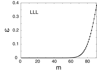
Figure 5: LLL reduced single-particle energies $\varepsilon$ as a function of the single-particle angular momentum $m=|l|$. Note the flat section of the curve that is followed by a rapid rise when the $\chi^{B}$ bulk-type component reaches the edge of the graphene sample. The graphene sample boundary is taken at $R=15l_{B}$. $\varepsilon$ is dimensionless (see text).

V Summary

We developed here a consistent picture of the many-body properties of interacting correlated Dirac electrons in graphene which is in correspondence with experimental findings pertaining to the incompressible FQHE states and insulating phase emerging at high magnetic fields. Key to the success of our theoretical model is the proper inclusion of the effect of the graphene-sample edge, treated here with the use of the zigzag boundary condition. This BC weights by a factor $1/\sqrt{2}$ the bulk-type wave functions in the two-component LLL Dirac spinor [Eq. (8)]; accounting for a 50% depletion of the bulk electron density. The other component (also weighted by $1/\sqrt{2}$) resides on the sample edge, leading to the emergence of an insulating phase.

These findings point to the unique role of the graphene edge in modulating the strength of the interelectron interactions governing the correlated many-body states in graphene, thus providing an impetus for future explorations, including controlled treatments of the graphene-sample boundaries.

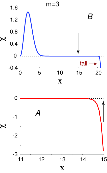
Figure 6: The two LLL orbital components $\chi^{B}(x)$ (marked as $B$, top frame) and $\chi^{A}(x)$ (marked as $A$, bottom frame) in Eq. (3) for $m=3$ ($l=-3$) and $x_{R}=15$ (a mixed bulk-edge DW spinor). The corresponding single-particle energy [see Eq. (4) and Fig. 5] is $\varepsilon=4.383\times 10^{-22}$. The vertical arrows at $x=x_{R}=R/l_{B}=15$ mark the position of the physical edge of the graphene sample. Inside the graphene sample ($x<x_{R}$), the $\chi^{B}$ component can be approximated by the bulk-type orbital in Eq. (5); outside the graphene sample ($x>x_{R}$), it develops an exponentially growing tail reflecting the fact that the full wave function in the entire range $0\leq x<\infty$ is described via a confluent hypergeometric function exhibiting a zero at $x=x_{R}$. The $\chi^{A}$ component is well represented by the edge orbital in Eq. (6).

Appendix A Solutions of the Dirac-Weyl equation in polar coordinates

The derivation of the solutions of the Dirac-Weyl Eq. (2) involves two subcases, i.e, for $\varepsilon\neq 0$ and $\varepsilon=0$.

For $\varepsilon\neq 0$, the solutions of Eq. (2) that are regular at the origin ($x=0$) can be found through the substitution of the following form in the DW equation,

$$\chi^{A}=Ce^{-x^{2}/4}x^{|l|}f_{l}(x),$$ (18)

which will specify $f_{l}(x)$.

For any $l$, and prior to invoking the zigzag boundary condition, the $\chi^{A}$ component is given by

$$\chi^{A}(x) = Ce^{-x^{2}/4}x^{|l|}\times$$ (19)

$$M\left(\frac{|l|+l}{2}+1-\frac{\varepsilon^{2}}{2},|l|+1,\frac{x^{2}}{2}\right).$$

In Eq. (19), $\varepsilon=E/(\hbar v_{F}/l_{B})$ is the reduced Dirac-electron energy, with $v_{F}$ the Fermi velocity and $l_{B}=(\hbar c/eB)^{1/2}$ the magnetic length. The general form of the $\chi^{B}$ component depends on whether $l$ is positive or negative, i.e.,

$$\chi^{B}(x)=-C\frac{2|l|}{\varepsilon}e^{-x^{2}/4}x^{|l|-1}M\left(-\frac{\varepsilon^{2}}{2},|l|,\frac{x^{2}}{2}\right),$$ (20)

for $l\leq-1$, and

$$\chi^{B}(x) = C\frac{\varepsilon}{2(l+1)}e^{-x^{2}/4}x^{l+1}\times$$ (21)

$$M\left(l+1-\frac{\varepsilon^{2}}{2},l+2,\frac{x^{2}}{2}\right),$$

for $l\geq 0$.

For $\varepsilon=0$, the two equations in the Dirac-Weyl system [Eq. (2)] decouple. In this case, the regular at the origin ($x=0$) solutions are:

$$\chi^{A}(x) = 0$$

$$\chi^{B}(x) = C^{B}x^{|l|-1}e^{-x^{2}/4},$$ (22)

for $l\leq-1$, and

$$\chi^{A}(x) = C^{A}x^{l}e^{x^{2}/4}$$

$$\chi^{B}(x) = 0.$$ (23)

for $l\geq 0$.

The interacting-electron EXD energies corresponding to these ($\varepsilon=0$) single-particle levels (taken as a basis) are higher than those resulting from the bulk-edge mixed states ($\varepsilon\neq 0$); consequently they correspond to excited states lying above the yrast band.

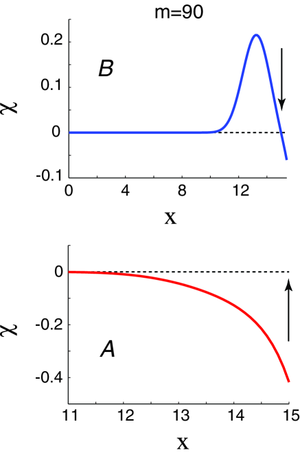
Figure 7: The two LLL orbital components $\chi^{B}(x)$ (marked as $B$, top frame) and $\chi^{A}(x)$ (marked as $A$, bottom frame) in Eq. (3) for $m=90$ ($l=-90$) and $x_{R}=15$ (a “double-edge” DW spinor, with both components representing edge-like orbitals). The corresponding single-particle energy [see Eq. (4) and Fig. 5] is $\varepsilon=0.349$. The vertical arrows at $x=x_{R}=R/l_{B}=15$ mark the position of the physical edge of the graphene sample. The $\chi^{B}$ component is similar to the nonrelativistic edge states familiar from the theory of the integer QHE in semiconductor heterostructures.halp82 The $\chi^{A}$ component is similar to the edge orbital in Eq. (6).

Appendix B Two different types of edge states

From early on, the concept of edge states has played a central role in the theory of the quantum Hall effect for nonrelativistic electrons.halp82 In addition to these nonrelativistic edge states, the sublattice struture of graphene (relativistic, Dirac electrons) allows in high $B$ for other unique types of edge states with no analog in nonrelativistic systems; in particular, the mixed (bulk-edge) states described by the spinor in Eq. (8). In this Appendix, we elaborate further on this point.

To this effect, it is instructive first to investigate the behavior of the LLL energies $\varepsilon\neq 0$ obtained as solutions of the transcendental equation (4). For a graphene sample with radius $R=15l_{B}$, the variation of the single-particle energies with $m=|l|$ is shown in Fig. 5. We observe a flat region where $\varepsilon$ is vanishingly small ($\varepsilon\sim 0$) transforming for higher angular momenta to a steeply rising branch. To gain insight into the nature of the single-particle levels in these two regions, we plot the two components of the Dirac-electron spinor for two characteristic angular momenta $m$.

In Fig. 6 we show the case of $m=3$ ($l=-3$, with $\varepsilon=4.383\times 10^{-22}$), which lies deep inside the flat region in Fig. 5. Inside the graphene sample ($x<x_{R}$), the $\chi^{B}$ component can be approximated by the bulk-type orbital in Eq. (5); outside the graphene sample ($x>x_{R}$), it develops an exponentially growing tail reflecting the fact that the full wave function in the expanded range $0\leq x<\infty$ is described via a confluent hypergeometric function exhibiting a zero at $x=x_{R}$. The $\chi^{A}$ component is well represented by the edge orbital in Eq. (6), and as aforementioned it does not have an analog for nonrelativistic LLL electrons.

We contrast this behavior by illustrating in Fig. 7 the spinor components corresponding to $m=90$ ($\varepsilon=0.349$) which is characteristic of the steeply rising branch in Fig. 5. The $\chi^{B}$ component is similar now to a nonrelativistic edge state familiar from the theory of the integer QHE in semiconductor heterostructures,halp82 while the $\chi^{A}$ component exhibits again a behavior similar to the edge orbital in Eq. (6).

From the above we conclude that the origin of the rising energy of the single-particle states with larger $m$ (see Fig. 5) reflects the shift of the centroid of the $\chi^{B}$ component toward the boundary while (simultaneously) satisfying the vanishing of this component on the sample boundary, thus disturbing the orbital shape (see Fig. 7). Note that the position of the centroid depends on $m$ (compare Figs. 6 and 7) and that $\langle x^{2}\rangle\approx 2(m+1)$ for $\sqrt{\langle x^{2}\rangle}<x_{R}$. Working in the regime $R/l_{B}>>1$, the states in the flat region of the energy curve in Fig. 5 form an effective LLL manifold composed of mixed bulk-edge single-particle spinors [approximated by the Dirac-electron spinor in Eq. (8)].

References

- (1) K.S. Novoselov et al., Science 306, 666 (2004).
- (2) K.S. Novoselov et al., Nature 438, 197 (2005).
- (3) Y. Zhang, Y.-W. Tan, H.L. Stormer, and Ph. Kim, Nature 438, 201 (2005).
- (4) C. Töke, P.E. Lammert, V.H. Crespi, and J.K. Jain, Phys. Rev. B 74, 235417 (2006).
- (5) V.M. Apalkov and T. Chakraborty, Phys. Rev. Lett. 97, 126801 (2006).
- (6) R.B. Laughlin, Phys. Rev. Lett. 50, 1395 (1983).
- (7) C. Yannouleas and U. Landman, Rep. Prog. Phys. 70, 2067 (2007); Phys. Rev. A 81, 023609 (2010).
- (8) J.K. Jain, Composite Fermions (Cambridge University Press, 2007).
- (9) X. Du, I. Skachko, F. Duerr, A. Luican, and E.Y. Andrei, Nature 462, 192 (2009).
- (10) K.I. Bolotin, F. Ghahari, M.D. Shulman, H.L. Stormer, and Ph. Kim, Nature 462, 196 (2009).
- (11) W. Bao et al., arXiv:1005.0033v1 (2010).
- (12) A.H. Castro Neto, F. Guinea, N.M.R. Peres, K.S. Novoselov, and A.K. Geim, Rev. Mod. Phys. 81, 109 (2009).
- (13) Using the high-precision capabilities of algebraic computer languages [see Ref. mathbook, ], we have checked numerically this equal-weight property. This property has been noted by L. Brey and H. A. Fertig [Phys. Rev. B 73, 195408 (2006)] in the context of a study of edge states of noninteracting Dirac electrons in a graphene ribbon. The equal-weight property is related to the particle-hole symmetry of the Dirac-Weyl equation (2). Indeed, it follows immediately that if (, ) are solutions of Eq. (2) with energy , then the pair (, ) is also a solution with opposite energy . For , this corresponds to two different spinor solutions of Eq. (2) which must be orthogonal; thus .
- (14) R. Peierls, Surprises In Theoretical Physics (Princeton University Press, Princeton, N.J., 1979), Ch. 3.6.
- (15) M. Abramowitz and I.A. Stegun (Editors), Handbook Of Mathematical Functions, (National Bureau of Standards, Washington, D.C., 1972).
- (16) See, e.g., S. Wolfram, Mathematica: A System for Doing Mathematics by Computer (Addison-Wesley, Reading, MA, 1991).
- (17) B.I. Halperin, Phys. Rev. B 25, 2185 (1982).
- (18) W. Gautschi and C. Giordano, Numer. Algor. 49, 11 (2008), in particular Sect. 3.2.3.
- (19) In particular formula 13.1.4 in Ref. abrabook, and the property that , .
- (20) R.B. Laughlin, Phys. Rev. B 27, 3383 (1983).
- (21) For , the excitation gaps calculated from Dirac electrons in a spherical geometry (i.e., boundless graphene) in Ref. jain06, are: (i) 0.042 (all energies are in units of ) [obtained from extrapolation of the (LLL) line in Fig. 1(c) in the above cited paper], and (ii) 0.017 for the extrapolated value calculated for the filling of the Landau level [see the label “” in Fig. 1(c)]. In both the and cases cited above, the gap involves composite-fermion pseudoskyrmions. The latter value (0.017) is the one cited in the experimental Ref. kim09, . Without consideration of pseudoskyrmion effects, the excitation energy gap at the filling of the Landau level calculated in the spherical geometry in Ref. chak06, [see Fig. 2(a) therein] for electrons is about 0.1 (see also Ref. jainbook, , Table 6.5, p. 185). Ref. andr09, cites this latter value (0.1) as the theoretically calculated one, noting that the measured excitation gap is 8% of this value. The value 0.0137 obtained from extrapolation of our LLL results for is lower in an essential way from all the theoretical values mentioned above, thus providing a potential signature for the edge-influenced depletion of the bulk Dirac-electron density.