Cu i resonance lines in turn-off stars of NGC 6752 and NGC 6397.

Abstract

Context. Copper is an element whose interesting evolution with metallicity is not fully understood. Observations of copper abundances rely on a very limited number of lines, the strongest are the Cu i lines of Mult. 1 at 324.7 nm and 327.3 nm which can be measured even at extremely low metallicities.

Aims. We investigate the quality of these lines as abundance indicators.

Methods. We measure these lines in two turn-off (TO) stars in the Globular Cluster NGC 6752 and two TO stars in the Globular Cluster NGC 6397 and derive abundances with 3D hydrodynamical model atmospheres computed with the CO5BOLD code. These abundances are compared to the Cu abundances measured in giant stars of the same clusters, using the lines of Mult. 2 at 510.5 nm and 578.2 nm.

Results. The abundances derived from the lines of Mult. 1 in TO stars differ from the abundances of giants of the same clusters. This is true both using CO5BOLD models and using traditional 1D model atmospheres. The LTE 3D corrections for TO stars are large, while they are small for giant stars.

Conclusions. The Cu i resonance lines of Mult. 1 are not reliable abundance indicators. It is likely that departures from LTE should be taken into account to properly describe these lines, although it is not clear if these alone can account for the observations. An investigation of these departures is indeed encouraged for both dwarfs and giants. Our recommendation to those interested in the study of the evolution of copper abundances is to rely on the measurements in giants, based on the lines of Mult. 2. We caution, however, that NLTE studies may imply a revision in all the Cu abundances, both in dwarfs and giants.

1 Introduction

There is no wide consensus on the nucleosynthetic origin of copper, and the complex picture drawn by the observations has no straightforward interpretation. Multiple channels can contribute to the production of this element. According to Bisterzo et al. (2004) there are five such channels: explosive nucleosynthesis, either in Type II supernovae (SNII) or in Type Ia supernovae (SNIa), slow neutron capture ($s-$process), either weak (i.e. taking place in massive stars in conditions of hydrostatic equilibrium during He and C burning) or main (i.e. occurring in the inter-shell region of low-mass asymptotic giant branch stars) and the weak $sr$-process. The latter occurs in massive stars in the C-burning shell when neutron densities reach very high values, intermediate between typical $s-$process neutron densities ($10^{9}-10^{11}$ cm^-3; Despain 1980) and $r-$process neutron densities ($10^{20}-10^{30}$ cm^-3; Kratz et al. 2007). The contribution of the $s-$process, both weak and main, to the solar system Cu abundance is estimated by Travaglio et al. (2004a) to be 27%. Explosive nucleosynthesis in SNII can account for 5% to 10% of the solar system Cu (Bisterzo et al., 2004). The contribution of SNIa is probably less well known, however, as pointed out by McWilliam & Smecker-Hane (2005), the available SNIa yields of Cu are rather low (Travaglio et al., 2004b; Thielemann et al., 1986). Bisterzo et al. (2004) claim that the bulk of cosmic Cu has indeed been produced by the weak $sr$-process.

Observations of copper abundances in Galactic stars show a decrease in the Cu/Fe ratio at low metallicities. This was first suggested by Cohen (1980), on the basis of the measurements in giant stars of several Globular Clusters of different metallicities (Cohen, 1978, 1979, 1980). It was not until the comprehensive study of Sneden et al. (1991) that this trend was clearly defined in a robust way, resting on measurements in a large sample of stars. Recent studies of field (Mishenina et al., 2002; Bihain et al., 2004) and Globular Cluster stars (Shetrone et al., 2001, 2003; Simmerer et al., 2003; Yong et al., 2005) have confirmed this trend (see Fig. 1 of Bisterzo et al., 2004). Somewhat at odds with these general results are the observations of the Globular Cluster $\omega$ Cen (Cunha et al., 2002; Pancino et al., 2002). Even though this cluster shows a sizeable spread in metal abundances ($-2.20\leq\rm[Fe/H]\leq-0.70$, Johnson et al., 2008), the Cu/Fe abundance ratio is nearly constant, with no discernible trend.

Observations in Local Group galaxies (Shetrone et al., 2001, 2003) show that metal-poor populations display low Cu/Fe ratios, similar to what is observed in Galactic stars of comparable metallicity. However, McWilliam & Smecker-Hane (2005) noted that the metal-rich population of the Sgr dSph displays considerably lower Cu/Fe ratios than Galactic stars of comparable metallicity. This result is confirmed by the measurements of Sbordone et al. (2007), who also include stars of the Globular Cluster Terzan 7, associated to the Sgr dSph.

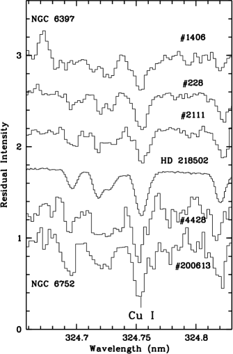
Figure 1: Cu i 324.7 nm line in the programme stars. The spectra are displaced vertically by 0.4 units, with respect to each other, for display purposes.

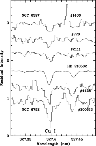
Figure 2: Cu i 327.3 nm line in the programme stars. The spectra are displaced vertically by 0.4 units, with respect to each other, for display purposes.

The majority of the Cu measurements are based on the Cu i lines of Mult. 2, sometimes one line of Mult. 7 is used. The exceptions are the measurements of Bihain et al. (2004) and Cohen et al. (2008), who use the resonance lines of Mult. 1 and Prochaska et al. (2000) who, to our knowledge, are the only ones who have made use of the strongest line of Mult. 6 in the near infrared. While for stars of metallicity above –1.0 one may have a choice of several lines to use, when going to metal-poor stars, for instance below –1.5, the only usable Cu abundance indicators are the two strongest lines of Cu i Mult. 2 in giant stars and the resonance lines of Mult. 1 in both dwarfs and giants. The advantage of the lines of Mult. 1 is that they are very strong, at high metallicity they are strongly saturated and therefore not ideal for abundance work, but, they remain measurable down to an extremely low metallicity. Bihain et al. (2004) have been able to measure the 327.3 nm line in the extremely metal-poor dwarf G64-12 ([Fe/H]$\sim-3$). Observationally the main disadvantage of Mult. 1 is that it lies in the UV, fairly near to the atmospheric cut-off. A very efficient UV spectrograph, like UVES and a large telescope, like VLT, may circumvent this problem. There are many spectra suitable for the measurement of the Cu i lines of Mult. 1 in stars of different metallicities in the ESO archive. The main purpose of our investigation is to assess the quality of the Cu i lines of Mult. 1 as abundance indicators. Our strategy is to compare for the first time Cu abundances in main sequence and giants of the same cluster, because Cu is not expected to be easily destroyed or created. This test will indicate the reliability of our modelling. Globular Clusters NGC 6397 and NGC 6752 span an interesting range in metallicity –2.0 to –1.5, which is relevant for a large fraction of the observations in field stars.

Table 1: Atmospheric parameters of the programme stars.

Star	Teff	$\log g$	[Fe/H]	$\xi$
	K	[cgs]	dex	$\mathrm{km\,s^{-1}}$
Cl* NGC 6752 GVS 4428	6226	4.28	-1.52	0.70
Cl* NGC 6752 GVS 200613	6226	4.28	-1.56	0.70
Cl* NGC 6397 ALA 1406	6345	4.10	-2.05	1.32
Cl* NGC 6397 ALA 228	6274	4.10	-2.05	1.32
Cl* NGC 6397 ALA 2111	6207	4.10	-2.01	1.32
HD 218502	6296	4.13	-1.85	1.00

2 Observations and equivalent width measurements

The spectra analysed here are the same as in Pasquini et al. (2004) and Pasquini et al. (2007) and described in the above papers. They were obtained with the UVES spectrograph (Dekker et al., 2000) at the ESO VLT-Kueyen 8.2m telescope. We here use the blue arm spectra, which are centred at 346 nm. Both clusters were observed with a $1^{\prime\prime}$ slit and a $2\times 2$ on-chip binning, which yields a resolution of about 40 000. The reduced spectra were downloaded from the ESO archive, thanks to the improved strategies for optimal extraction (Ballester et al., 2006), the S/N ratios are greatly improved compared to what was previously available. The equivalent widths (EWs) of the two Cu i lines of Mult. 1 were measured with the IRAF task splot and are provided in the on-line Table 6.

In addition to the four cluster stars we analyse the field star HD 218502 as a reference. Its atmospheric parameters are close to those of the cluster stars. For this star we work with the data used by Pasquini et al. (2004) as well as with the data observed in 2005, in the course of ESO programme 76.B-0133 (see Smiljanic et al., 2008). For this star we used six spectra: two with 1$\aas@@fstack{\prime\prime}$0 and $2\times 2$ binning, two with 1$\aas@@fstack{\prime\prime}$0 and $1\times 1$ binning, two with 1$\aas@@fstack{\prime\prime}$2 and $1\times 1$ binning. Each pair of spectra was coadded, the equivalent widths were measured on the coadded spectrum and then the three equivalent widths were averaged. The spectra of all the five stars analysed here are shown in Fig. 1 and 2.

One of the goals of the present analysis is to compare the Cu abundances in the TO stars with those measured in giant stars of the same cluster. For NGC 6752 we can rely on the recent analysis by Yong et al. (2005), who analysed 38 giants in this cluster, making use of high-resolution high-S/N ratio UVES spectra. The atomic data used by Yong et al. (2005) are the same as those here used. The analysis is based on 1D ATLAS models and LTE spectrum synthesis. That the ATLAS models employed by Yong et al. (2005) use the approximate overshooting option in ATLAS, while those we use do not, brings about only minor differences. Thus the measurements of Yong et al. (2005) are directly comparable to our own. The measurements of Yong et al. (2005) are, however, based only on the strongest line of Mult. 2. Because we aim to compare the abundance derived from the lines of Mult. 1 and Mult. 2 we retrieved UVES reduced spectra of one of the stars of Yong et al. (2005) from the ESO archive: Cl* NGC 6752 YGN 30. We used three spectra of 1800 s obtained with the dichroic # 1, the blue arm spectrum was centred at 346 nm and the red arm spectrum at 580 nm. The slit was set at 1$\aas@@fstack{\prime\prime}$0 in the blue arm and 0$\aas@@fstack{\prime\prime}$7 in the red arm; the CCD binning was $1\times 1$ for both arms. The corresponding resolution is $\sim 45\,000$ for the blue arm and $\sim 60\,000$ in the red arm.

For the cluster NGC 6397, though, we were unable to find any recent analysis that included the measurement of Cu. In fact the only measurement of Cu in this cluster which we could find is due to Gratton (1982). In order to make the Gratton (1982) measurements directly comparable to our own we used the published EWs of the Cu i lines of Mult. 2 and derive the abundances with our models, spectrum synthesis codes, and atomic data.

3 Cu abundances

3.1 Atomic data

To determine the Cu abundances for the TO stars we used the Cu i resonance lines of Mult. 1 at 324.7  nm and 327.3  nm. The $\log gf$ values were taken from Bielski (1975) and the hyperfine structure and isotopic shifts for the ⁶³Cu and ⁶⁵Cu isotopes from Kurucz (1999). We used the same sources for the two lines of Mult. 2 at 510.5  nm and 587.2 nm that we used for the giant stars. The line list used for the computations is given on-line in Table 5. The line at 327.3  nm is free from blends in metal-poor TO stars and the continuum is usually easily determined. The stronger 324.7  nm line, though, lies in a more complex spectral region. The only truly blending feature is a weak OH line (324.7615 nm), but, the line is on the red wing of a complex blend, mainly of iron lines, of which several have poor $\log gf$ values. The continuum is more difficult to determine for this line, given the larger line crowding in this region. We experimented with different choices for the Van der Waals broadening of the lines, the ABO theory (Anstee & O’Mara, 1995; Barklem & O’Mara, 1997; Barklem et al., 1998a, b) and the WIDTH approximation (Kurucz 1993a, 2005; Castelli 2005, see also Ryan 1998). For the transitions under consideration the WIDTH approximation and the ABO theory yield almost identical values.

3.2 Atmospheric parameters

The adopted atmospheric parameters for our programme stars are given in Table 1 and were taken from Pasquini et al. (2004) and Pasquini et al. (2007). For the giant star Cl* NGC 6752 YGN 30 we adopted the atmospheric parameters of Yong et al. (2005). For the two giants in NGC 6397 we adopted the atmospheric parameters of Gratton (1982). For the reader’s convenience the atmospheric parameters of the giant stars are provided here on-line in Table 7.

3.3 Model atmospheres and spectrum synthesis.

For each star we computed a 1D model atmosphere using version 9 of the ATLAS code (Kurucz, 1993a, 2005) under Linux (Sbordone et al., 2004; Sbordone, 2005). We used the opacity distribution functions described by Castelli & Kurucz (2003) and microturbulent velocity 1  $\mathrm{km\,s^{-1}}$, the mixing-length parameter, $\alpha_{\mathrm{MLT}}$, was set to 1.25, and the overshooting switched off. This model atmosphere was used as input to the SYNTHE code (Kurucz, 1993b, 2005), with different Cu abundances, to compute a curve-of-growth for each line. The Cu abundances were derived by interpolating in these curves of growth. The corresponding abundances are given in the second column of Table 2, the $\sigma$ is the variance of the abundances of the two lines. The abundances for the individual lines can be found on-line in Table 6.

The use of three dimensional hydrodynamical simulations to describe stellar atmospheres (hereafter 3D models) has led to the important notion that the outer layers present steeper temperature gradients than predicted by traditional 1D static model atmospheres (Asplund et al., 1999; Asplund, 2005; González Hernández et al., 2008) and that this effect is considerably more pronounced for metal-poor stars. In addition to the different mean temperature profile, the 3D models differ from traditional 1D models because they account for the horizontal temperature fluctuations. Both effects may or may not be important, depending on the line formation properties of the transition under consideration. In order to investigate these effects for the Cu i lines we used several 3D models computed with the code CO⁵BOLD (Freytag et al., 2002, 2003; Wedemeyer et al., 2004). The characteristics of the 3D models employed in this study are given in Table 3. The line formation computations for the 3D models were performed with the Linfor3D code. For each 3D model we used also two reference 1D models: the $\left\langle\mathrm{3D}\right\rangle$ and the $\mathrm{1D}_{\mathrm{LHD}}$, which we define below.

The $\left\langle\mathrm{3D}\right\rangle$ models are computed on-the-fly by Linfor3D by averaging the 3D model over surfaces of equal Rosseland optical depth and time. The $\left\langle\mathrm{3D}\right\rangle$ model has, by construction, the mean temperature structure of the CO⁵BOLD model, therefore the difference in abundance A(3D)-A($\left\langle\mathrm{3D}\right\rangle$), allows us to single out the effects caused by temperature fluctuations (see Caffau & Ludwig, 2007).

The $\mathrm{1D}_{\mathrm{LHD}}$ model is a 1D, plane parallel, LTE, static, model atmosphere and employs the same micro-physics and opacity as the CO⁵BOLD models; it is computed with the LHD code. These models are our models of choice to define the “3D correction” as A(3D) - A($\mathrm{1D}_{\mathrm{LHD}}$), where A is the abundance of any given element. More details on the LHD models may be found in Caffau & Ludwig (2007) and Caffau et al. (2010).

In any given Linfor3D run we made computations also for the $\left\langle\mathrm{3D}\right\rangle$ model and for a $\mathrm{1D}_{\mathrm{LHD}}$ model, with the same T_eff, log g, and metallicity as the 3D model.

Figure 3: Curves of growth (COG) for the Cu i 327.3 nm transition. The dotted line to the left is the COG for the 3D model d3t63g40m20n01, the three solid lines to the right are those for the corresponding $\mathrm{1D}_{\mathrm{LHD}}$ model for three values of the microturbulent velocity: 0.5, 1.0 and 1.5  $\mathrm{km\,s^{-1}}$, bottom to top. The dashed line is the 3D COG shifted arbitrarily by +0.58 dex along the x-axis. This highlights that the shape of the 3D COG differs from that of the corresponding 1D COGs and therefore the 3D correction depends on the EW of the transition.

Table 2: Copper abundances for the programme stars.

Star	A(Cu)	$\sigma$	A(Cu)	$\sigma$
	1D		3D
Cl* NGC 6752 GVS 4428	3.23	0.08	2.56	0.16
Cl* NGC 6752 GVS 200613	3.01	0.05	2.23	0.07
Cl* NGC 6397 ALA 1406	1.33	0.03	0.74	0.05
Cl* NGC 6397 ALA 228	1.30	0.03	0.73	0.05
Cl* NGC 6397 ALA 2111	1.19	0.02	0.60	0.02
HD 218502	1.52	0.09	0.95	0.04

Table 3: CO⁵BOLD models employed in the study.

Model	Teff	log g	[M/H]	$N_{\mathrm{t}}$	time	$t_{\mathrm{c}}$	Resolution	Box Size
	K				s	s		${\rm Mm}^{3}$
d3t50g25mm10n01	4990	2.5	$-1.0$	20	475990	1411.9	$160\times 160\times 200$	$573.2\times 573.2\times 245.4$
d3t50g25mm20n01	5020	2.5	$-2.0$	20	403990	1388.3	$160\times 160\times 200$	$584.0\times 584.0\times 245.4$
d3t63g40mm10n01	6260	4.0	$-1.0$	20	43800	12.2	$140\times 140\times 150$	$26.0\times 26.0\times 12.8$
d3t63g40mm20n01	6280	4.0	$-2.0$	16	27600	49.0	$140\times 140\times 150$	$26.1\times 26.1\times 12.8$
d3t63g45mm10n01	6240	4.5	$-1.0$	20	24960	16.0	$140\times 140\times 150$	$7.0\times 7.0\times 4.0$
d3t63g45mm20n01	6320	4.5	$-2.0$	19	9120	15.9	$140\times 140\times 150$	$7.0\times 7.0\times 4.0$

Table 4: Mean copper abundances for the two clusters.

Star	A(Cu)	$\sigma$	A(Cu)	$\sigma$
	1D		3D
NGC 6752 dwarfs	3.04	0.07	2.28	0.12
NGC 6752 giants	2.03	0.05	1.98	0.05
NGC 6397 dwarfs	1.25	0.05	0.63	0.04
NGC 6397 giants	1.40	0.17	1.30	0.17

The computation of a 3D model is still very time consuming, even on modern computers (several months), it would be impractical to compute a specific 3D model for any set of our atmospheric parameters. Our strategy is therefore the following: we perform an abundance analysis with ATLAS model atmospheres computed for the desired set of atmospheric parameters; we use a grid of 3D models with atmospheric parameters that bracket the desired ones and compute the relevant 3D corrections by linear or bi-linear interpolation in the grid, as appropriate; the 3D abundance is obtained by applying the interpolated 3D correction to the 1D abundance.

The line formation computations were performed using SYNTHE for the ATLAS models and Linfor3D for all other models. As a consistency check we used Linfor3D with an ATLAS model as input and verified that the line profiles and EWs are consistent with the results derived from SYNTHE+ATLAS. The difference between the two line formation codes amounts to a few hundredths of dex in terms of abundance, a quantity that is irrelevant with respect to the size of the 3D corrections under consideration.

For three out of the six TO stars under study, the Cu i lines are strong (EW$>4.0$ pm), therefore they are surely in the saturation regime. Their 3D correction depends on the adopted microturbulence in the adopted reference 1D atmosphere. To take this into account, different $\mathrm{1D}_{\mathrm{LHD}}$ curves of growth were computed with microturbulent velocities of 0.5, 1.0 and 1.5  $\mathrm{km\,s^{-1}}$, to allow us interpolation to any desired value of $\xi$. For weaker lines the microturbulent velocity does not play a fundamental rule, so that the 3D correction is mostly insensitive on the choice of this parameter. We find that the 3D curve of growth is not a simple translation of a 1D curve of growth, but has a distinct shape. An example to illustrate the effect is shown in Fig. 3. An immediate consequence is that for all lines we considered, the 3D correction depends on the EW, even for the weaker lines. We note that the dependence of the 3D correction on the microturbulence implies that the abundance obtained by applying the correction to an abundance derived from a 1D model depends on the adopted microturbulence. One of the reasons to prefer the use of 3D models is to avoid the use of this parameter. The correct way to treat this is, not to use the 3D correction, but to derive the abundance by an interpolation in a set of 3D curves of growth, or to use suitable fitting functions, as done for lithium by Sbordone et al. (2010). But this requires the use of a larger set of 3D models, which bracket the effective temperatures of the studied stars. For the purpose of the present exploratory investigation we believe the approach of using 3D corrections is adequate, especially because the conclusion of the study is that 3D-LTE abundances are unreliable. Finally we point out that it may be that current 3D models do not correctly capture turbulence at small scales (Steffen et al., 2009). If this were indeed the case all abundances derived from saturated lines are doubtful, whether they are derived applying a 3D correction or directly derived from the 3D curves of growth.

We therefore computed the 3D correction for each of the measured EWs for each of the relevant 3D models. In general the 3D correction will also depend on the treatment of convection in the 1D reference model, hence on the adopted $\alpha_{\mathrm{MLT}}$. The lines under consideration do not form in the deepest layers, which are the most affected by the choice of $\alpha_{\mathrm{MLT}}$, thus they are insensitive to it. All $\mathrm{1D}_{\mathrm{LHD}}$ models employed have $\alpha_{\mathrm{MLT}}$= 1.0. The computed A(3D) – A($\mathrm{1D}_{\mathrm{LHD}}$) corrections, as well as the A(3D) – A($\left\langle\mathrm{3D}\right\rangle$) corrections are given on-line in Table 8. The 3D abundances provided in Table 2 are obtained by applying to the 1D abundances the 3D corrections in Table 6, which were obtained by interpolating the corrections in Table 8.

The six stars under study have very similar effective temperatures. All are within roughly 100 K of the effective temperatures of the 3D models listed in Table 3 (T_eff$\sim 6300$ K). Therefore it is not necessary to include more 3D models and perform an interpolation in T_eff. The metallicities and gravities of the models in Table 3 bracket the metallicities and gravities in Table 1. We used a bi-linear interpolation in metallicity and gravity for the two stars of NGC 6752 and for HD 218502. The three stars of NGC 6397, though have a metallicity of almost –2.0, therefore a linear interpolation in surface gravity was sufficient.

The computation of 3D models for typical giant stars is much more time consuming than for F-type and cooler dwarfs. The radiative relaxation time in the surface layers of warm giants becomes significantly shorter than the dynamical time scale, which makes it computationally expensive to properly capture the time evolution of the system. At present we have only two fully relaxed models of metal-poor giants. The parameters are given in Table 3 and the metallicities are –1.0 and –2.0. The surface gravity is larger than that of the majority of the giant stars analysed in either cluster. Only the faintest stars analysed by Yong et al. (2005) have parameters T_eff and log g close to those of our giant models. In spite of this we believe that we can use the 3D corrections derived from this model, as a first order approximation as representative of the corrections in giant stars of both clusters. This is possible because the 3D corrections are rather small, especially when compared to those of dwarf stars. This is partly because giant 3D models do not show a pronounced over-cooling, compared to 1D models, as dwarfs display. This conclusion is also based on the examination of several snapshots of not fully relaxed giants of different atmospheric parameters, which we are in the process of computing. The 3D correction for the giant models is –0.1 dex for both the examined Cu i lines of Mult. 2 for the model of metallicity –2.0 and 0.0 dex (actually +0.01) for the model of metallicity –1.0. We apply a correction of –0.1 to the abundances of giant stars in NGC 6397 and –0.05 to those of NGC 6752.

Figure 4: Contribution functions of the EW at disc-centre, defined in a way that their integral over $\log\tau_{\lambda}$ gives the EW (Magain, 1986), for the Cu i 324.7 nm line and the model d3t63g40mm20n01 for two different values of Cu abundance. In the upper panel A(Cu)=0.2, in the lower panel A(Cu)=1.7. The solid lines refer to the 3D model, the dashed lines to the corresponding $\mathrm{1D}_{\mathrm{LHD}}$ model.

Figure 5: Contribution functions for the Cu i 510.5 nm line and the model d3t50g25mm20n01. The solid line refers to the 3D model, the dashed line to the corresponding $\mathrm{1D}_{\mathrm{LHD}}$ model.

4 Results

4.1 HD 218502

The analysis of the reference star HD 218502 shows that the abundances derived from the two Cu i resonance lines (Table 6) agree well, both with 1D and 3D models. This gives us confidence in the reliability of the atomic data used. It also suggests that with good quality data, the EWs of both lines can be satisfactorily measured in spite of the complexity of the spectral region, especially for the 324.7 nm line. Our 1D abundance (A(Cu)$=1.52\pm 0.09$) agrees, within errors with what reported by Bihain et al. (2004, A(Cu)$=1.70\pm 0.17$). We note a small difference in the effective temperature adopted in the two analyses (about 100 K) and a difference in the data: our UVES spectra are of considerably higher quality than the CASPEC spectra used by Bihain et al. (2004), who measured only the 327.3 nm line. This agreement is expected because the atomic data are the same in the two analyses and the 1D model atmospheres used are similar, the main difference being the overshooting. This check suggests that we may reasonably assume that our Cu abundances should be consistent with those of Bihain et al. (2004), which are based on the UV resonance lines. An inspection of Fig. 6 of Bihain et al. (2004) suggests that these measurements substantially agree with those of Mishenina et al. (2002), which are essentially based on the measurements of the lines of Mult. 2. Yet one should take into account the large error bars that derive from the relatively poor S/N ratio that is achievable in the UV range.

The 3D correction for the lines of Mult.1 is large and the 3D abundance in this star is well below all the measurements in giant stars of similar metallicity. An application of 3D corrections to all measurements of Bihain et al. (2004) would probably break the agreement with the measurements of Mishenina et al. (2002). We have inspected the available red spectra of HD 218502, to see if any of the lines of Mult. 2 could be detected, but this was not the case.

4.2 TO stars in NGC 6752 and NGC 6397

For the cluster stars there is also a good consistency between the abundances derived from the two resonance lines for any given line, in spite of the much lower S/N ratios in the cluster stars. This suggests that there is no major inconsistency in the EW measurements.

The weighted mean of the abundances of the clusters, reported in Table 4, displays an error in the mean that is reasonably small. We believe that the mean abundances for the two clusters obtained from the dwarf stars are indeed representative of the Cu i abundance derived from the lines of Mult. 1. Considering that each spectrum of a TO star in these clusters amounts to about 10 hours of integration with UVES, it is unlikely that in the near future better data or data for a larger number of stars will be available, although it would clearly be desirable.

4.3 Star Cl* NGC 6752 YGN 30

In this star, like in the other giant stars observed by Yong et al. (2005), both the lines of Mult. 1 and of Mult. 2 are measurable, which provides for a consistency check. We did not measure the line at 324.7 nm since the region is extremely crowded in these cool giants, but the line at 327.3 nm is clean and unblended. For Mult. 2 we only measured the 510.5 nm line, since the other line is not present in the spectrum, because it falls in the gap between the two CCDs. The two lines (324.7 nm and 510.5 nm ) provide inconsistent results, the line of Mult. 1 provides an abundance that is 0.54 dex higher than that of the line of Mult. 2 (see on-line Table 6). The abundance we derive from the line of Mult. 2 substantiallly agrees with the measure of Yong et al. (2005), our abundance is 0.13 dex smaller. Of this difference 0.05 dex are because we use ATLAS models without overshooting, while Yong et al. (2005) use models with overshooting, the remaining difference should be attributed to a difference in the measured EW and possibly to the different spectrum synthesis codes used (MOOG by Yong et al. 2005 and SYNTHE by us). The 3D corrections for both lines of Mult. 1 and Mult. 2 are small and agree to within a few hundredths of dex. The abundance from the two lines cannot be brought into agreement by using 3D models.

4.4 Giant stars in NGC 6397

The error in the mean of the two giants is 0.18 dex, which is essentially identical to the estimate of Gratton (1982) of 0.2 dex on the copper abundance. Even making use of 1D models the abundance of the giant stars is considerably higher than in the dwarf stars.

5 Effects of atmospheric parameters

We intend to quantify the effect of changing atmospheric parameters on the derived abundances. The abundances derived from the Cu i resonance lines are fairly sensitive, for a neutral species, to the adopted surface gravity. For dwarf stars a change of $\pm 0.25$  dex in log g induces a change of $\mp 0.1$ dex in abundance. For the giant stars they are only slightly less sensitive, $\mp 0.06$ dex. On the other hand for giant stars the dependence on gravity of the abundances derived from the lines of Mult. 2 is very weak $\mp 0.01$ dex. An inspection of on-line Table 8 allows us to estimate the effect of surface gravity on the 3D corrections for the lines of Mult. 1. By increasing the gravity by 0.5 dex, the 3D correction increases by 0.1 to 0.2 dex, depending on how saturated the line is. Since the 3D correction is negative, this means that it decreases in absolute value. The opposite trends with surface gravity on the 1D abundance and 3D correction imply that the two effects tend to cancel and the overall sensitivity of the 3D abundance on surface gravity is small.

The dependence of abundances on effective temperatures for the lines of Mult.  1 is similar for dwarfs and giants, and is about $\pm 0.2$ dex for a change of $\pm 100$ K in effective temperature. To evaluate the dependence of the 3D corrections on the effective temperature we used four models, extracted from the CIFIST grid (Ludwig et al., 2009). All four models have effective temperature around 5900 K, their metallicities are –1.0 and –2.0 and their log g 4.0 and 4.5. The result is that for a decrease of 300  K the 3D correction increases by 0.2 dex. Again the variation of the 3D correction goes in the opposite direction with respect to the variation in the 1D abundance. Combining the results we conclude that a decrease of 300 K in effective temperature results in a decrease by 0.4 dex in copper abundance (3D).

For the giants stars we also estimated the variation of the abundances derived from the lines of Mult.  2, which amounts to about $\pm 0.1$ dex for a variation of $\pm 100$ K in effective temperature.

6 Hydrodynamical models and spectrum synthesis.

Clearly the large 3D corrections derived for the Cu i resonance lines are driven by the fact that in the outer layers the hydrodynamical models are considerably cooler than the corresponding 1D models, the so-called “overcooling”. This shifts the ionisation equilibrium towards neutral copper, and as a consequence the line contribution function shows a strong peak in these layers, contrary to the 1D model (se Fig. 4). From a physical point of view this is expected, simply because the hydrodynamical model is observed to transport flux through convection even in layers where the corresponding 1D model is formally stable against convection (overshooting). One should however ask to which extent the computed overcooling depends on the assumptions made. Bonifacio (2010) pointed out the difference in the overcooling for metal-poor giants computed with CO⁵BOLD and that computed by Collet et al. (2007). Behara et al. (2009) pointed out that for extremely metal-poor dwarfs the overcooling is considerably less in CO⁵BOLD models computed with 12 opacity bins than in models computed with 6 opacity bins, like the ones used here.

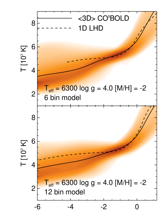
Figure 6: Comparison between the temperature structures of two models with T_eff= 6300, log g= 4.0 and metallicity –2.0, computed with 6 and 12 opacity difference. The difference is not as large as it is at lower metallicities (see Fig. 1 of Behara et al. 2009).

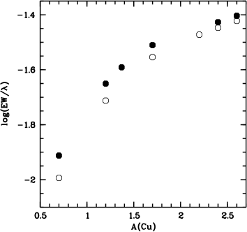
Figure 7: Comparison between the curves of growth for the 327.3 nm line computed for the two models shown in Fig. 6. Solid symbols correspond to the 6 bin model and open symbols to the 12 bin model.

For the time being we have relatively few CO⁵BOLD models computed with 12 opacity bins, among which we have one with parameters identical to one used in the present investigation: T_eff= 6300, log g= 4.0 and metallicity = –2.0. In Fig. 6 we show the mean temperature structures of the two models. Obviously the difference is smaller than what is displayed by the models 1 dex more metal-poor shown by Behara et al. (2009). The qualitative conclusion is confirmed by comparison of the curves of growth. In Fig. 7 the curve of growth for the 327.3 nm line used in the present investigation is compared to the one computed from the corresponding 12 bin model. As can be appreciated from the plot, for a given equivalent width the 12 bin model will yield a Cu abundance that is higher by approximately 0.1 dex, thus correspondingly decreasing the 3D correction.

Another matter of concern is that the current version of Linfor3D treats scattering as true absorption. That is to say, although scattering processes such as Rayleigh scattering off hydrogen atoms are taken into account as opacity sources, in the solution of the transfer equation the source function is set equal to the local Planck function, without a term depending on the mean radiation intensity ($S_{\nu}=B_{\nu}$). To which extent can this approximation affect our computations, especially in the near ultraviolet, where scattering processes are a non-negligible source of opacity ? We assessed this by using 1D models and 1D spectrum synthesis. We used a slightly modified version of the SPECTRV code in the SYNTHE suite so that scattering is treated as true absorption when the card SCATTERING OFF is set in the input model (see e.g. Castelli 1988). We computed line profiles both with SCATTERING ON and SCATTERING OFF for the model at T_eff= 6296 K log g= 4.0 and metallicity –2.0 (rlevant to HD 218502) and for the model T_eff= 4943 log g= 2.42 and metallicity –1.5 (relevant to Cl* NGC 6752 YGN 30). It turns out that in both cases the difference is irrelevant to our analysis (0.6% in the continuum and 0.03% in the residual intensity for the dwarf model and 14% in the continuum and 2% in the residual intensity). The effect of treating scattering as true absorption is very similar on the continuum and in the lines, thus implying a small effect on the residual intensity and equivalent width.

Recently Hayek et al. (2010) have introduced a proper treatment of scattering in their magneto-hydrodynamical simulation code, BIFROST. For the Sun and solar-type stars they do not find a significant impact of continuum scattering on the temperature structure. We thus believe that although the impact of a proper treatment of scattering needs to be investigated in metal-poor dwarfs, it seems unlikely that the results presented here will be seriously challenged by this.

7 Discussion

If we consider the abundances in Table 4 at face value we are led to the inescapable conclusion that the Cu abundances in dwarfs and giants do not agree. Even though the abundances are almost compatible, within errors, at least in the 1D case, this systematic difference should not be overlooked. The behaviour is different between the two clusters: in NGC 6752 the dwarfs provide a higher abundance than the giants, while in the case of NGC 6397, they provide a lower value than the giants; this both using 1D and 3D models. For NGC 6752 the difference in 1D abundances is of one order of magnitude (1 dex), but this is reduced to only 0.3 dex if we look at the 3D abundances, which are almost compatible with the errors. The situation is reversed in NGC 6397, in 1D the abundances of dwarfs is only 0.15  dex lower than that in giants, while in 3D, the diferece is 0.9  dex. This behaviour may be understood in terms of the different line formation properties in dwarfs and giants and how they change with different Cu abundance. In Fig. 4 we show, as an example, the contribution functions of the EW at disc-centre for one of our models for a dwarf star, for two different Cu abundances. In the top panel A(Cu)=0.2 and the line is on the linear part of the curve of growth, in the bottom panel, A(Cu)=1.7 and the line is saturated. In both cases the 3D contribution function is very different from the 1D one and is peaked in the outer layers of the atmosphere. The formation of the lines of Mult. 2 in the atmospheres of giants is instead much less affected by 3D effects, as depicted in Fig. 5. The contribution functions of the lines of Mult. 1 in the giant model are morphologically similar to what is shown in Fig. 5, confirming the weak overcooling present in this model. While the above arguments explain the behaviour of the 3D corrections, they have no bearing in the abundance difference that we find between dwarfs and giants.

In these situations one has always to consider two possible alternatives: i) the difference is true and has an astrophysical origin; ii) the difference arises from shortcomings in the analysis. In our opinion hypothesis i) must be discarded. It seems extremely far fetched to devise a physical mechanism by which Cu should be overabundant in dwarf stars, like in NGC 6752, while the reverse is true in NGC 6397. Where giants have a higher Cu abundance, one could imagine to explain such a scenario either by invoking diffusion in TO stars, or Cu production in giant stars, or perhaps even a combination of both. However, an examination of Table 4 shows that the differences that need explanation are far too large to be created by diffusion, and the Cu production would also have to be highly efficient. In addition note that the Cu abundances in the large sample of Yong et al. (2005) are extremely uniform, which speaks against Cu production.

Thus we are left with the conclusion that the abundance determinations in either dwarfs or giants, or both, are wrong. Let us start by examining the 3D abundances in dwarf stars. Contribution functions like those shown in Fig. 4 must give rise to concerns about the LTE approximation used in our computations. The outer and less dense layers of the atmosphere, which contribute mostly to the line EW, are those in which the photon mean free path is longest and deviations from LTE may be expected. The situation is even more extreme in a 3D atmosphere where photons from a hot up-draft may transfer horizontally and overionise a neighbouring cool down-draft. A morphologically similar situation is indeed observed for the Li i doublet in metal-poor stars (Asplund et al., 2003; Cayrel et al., 2007). In LTE the contribution function displays a double peak, with a substantial contribution from outer cool layers, in NLTE this peak is entirely suppressed by overionisation. The nearly exact cancellation between 3D and NLTE correction that takes place for the Li i doublet, and results in 3D-NLTE abundances in very close agreement with 1D-LTE abundances, should not be taken as a general rule. Nevertheless we believe that the Cu i lines of Mult. 1 cannot be described by 3D-LTE computations, but NLTE effects should be properly accounted for.

This leads to the question of how reliable the LTE approximation is for the 1D computations. That even in 1D the abundances in dwarfs and giants differ by a factor of the order of 2, surely prompts to see if for NLTE computations the two sets of abundances may be brought into agreement. Bihain et al. (2004) tried to fit the Cu i lines of Mult. 1 in the solar spectrum, but were unable to reproduce the core of the lines. This was attributed mainly to the presence of a chromosphere that influences the cores of strong lines. Deviations from LTE, however, could be another, possibly concomitant, cause for the failure to reproduce the line core in LTE. For Pop II dwarf stars chromospheric effects should not be strong, in view of their old age, even if chromospheres were present.

Let us finally consider the Cu abundances in giant stars. Our limited computations suggest that they should not suffer large 3D effects. The test we conducted for the giant star in NGC 6752 suggests that the LTE synthesis does not allow us to reproduce satisfactorily the lines of Mult. 1 and of Mult. 2 with the same Cu abundance. Indeed the discrepancy is quite large (0.5 dex); significant deviations from LTE for either or both sets of lines could be responsible for this. Which should be further investigated in order to produce reliable Cu abundances. The evolution of copper with metallicity, essentially based on the measurements of Mult. 2 in giant stars, shows a rather sharp drop in [Cu/Fe] around [Fe/H]=–1.5. This means that it takes place around A(Cu)=2.0. In the curve of growth for the 510.5 nm line of Mult. 2 for our giant model, this is roughly the abundance for which the line begins to enter in the saturation regime. If the Cu i lines of Mult. 2 suffer deviations from LTE it is likely that these depend on the line strength and may show a rather sharp change just when the line enters a saturation regime. This behaviour is observed, for instance, for the sodium D lines (see Fig. 6 of Andrievsky et al., 2007). These considerations render NLTE computations for Cu very desirable.

Unfortunately, to our knowledge, up to now no such computations have been published, nor does a Cu model atom exist.

Among the possible causes for the discrepancy in abundances between giants and dwarfs one may also consider errors in the atmospheric parameters. One may conclude that this cannot be the case by noticing the discrepancy between the Cu abundance derived from Mult. 1 and Mult. 2 in star Cl* NGC 6752 YGN 30, for which lines of both multiplets are measured. Given that the response of both multiplets to a change in effective temperature is similar, the conflicting results cannot be resolved by changing the effective temperature. Of course the discrepancy between the two multiplets can be resolved in 1D by invoking a higher microtrubulence, but it would be necessary to raise it by 1  $\mathrm{km\,s^{-1}}$. This increase would then cause a strong trend between iron abundances and equivalent widths. Furthermore this would not allow us to solve the discrepancy in the 3D analysis. Indeed while the 3D correction for Mult. 2 would not change significantly with this increase in microturbulence, those of Mult. 1 would increase by about 0.4 dex, thus breaking the agreement between the two multiplets forced in 1D. Formally one can certainly find a value of the microturbulence that forces the 1D abundance plus 3D correction of the two mutliplets to be equal, while leaving a discrepancy in the 1D abundances. This however would again cause an abundance spread among lines of other elements (e.g. iron) and can hardly be invoked as a solution of the problem. Although at the moment we do not have enough 3D models for giant stars to perform a full 3D analysis, as done by Sbordone et al. (2010) for lithium, we believe that our results indicate that this analysis will provide discrepant abundances from the two multiplets.

Let us further consider if changes in the atmospheric parameters of giant or dwarf stars in either cluster may allow us to reconcile their copper abundances. As discussed in Sect. 5 a decrease in effective temperature of 300 K in dwarf stars implies a decrease by about 0.4 dex. Therefore for the dwarf stars in NGC 6752 a decrease in effective temperature by about 225 K while keeping the temperature of giants constant, would reconcile the copper abundances of the to sets of stars. While not implausible, this change would certainly cause a mismatch in the abundances of other elements between giants and dwarfs, most notably iron, which would become less abundant in dwarfs than in giants. While one could argue that atmospheric phenomena such as diffusion may alter abundances of dwarf stars, it seems then contrived to invoke a different behaviour between copper and iron. But let us now turn to the other cluster, NGC 6397. Here the situation is reversed, the dwarfs display a lower abundance than giants. However here one would need to invoke an increase in effective temperatures of the dwarf stars by over 500 K, placing them at T_eff around 6700 K and the cluster turn-off at about 6900 K. While these exceedingly high temperatures may be appealing (one would immediately solve the cosmological lithium problem!) they appear impossible to reconcile with the colours of the cluster and theoretical isochrones.

Although the precise value of the atmospheric parameters assigned to the stars certainly plays a role in the difference in copper abundances between dwarfs and giants in the two clusters, we may dismiss the hypothesis that it may be cancelled by a suitable choice of parameters.

8 Conclusions

Our study of the Cu i lines of Mult. 1 in the TO stars of the globular clusters NGC 6397 and NGC 6752 allow us to draw several conclusions:

1. the Cu abundance derived from the Cu i lines of Mult. 1 in dwarf stars differs from that derived in giants from the Cu i lines of Mult. 2 in the same clusters;

2. the Cu i lines of Mult. 1 in dwarf stars show large 3D corrections when computed in LTE;

3. the Cu i lines of Mult. 2 in giant stars show small 3D corrections when computed in LTE;

4. the contribution functions of the Cu i lines of Mult. 1 in dwarf stars suggest that these cannot be reliably computed under the LTE approximation;

5. for the only star for which we have measured both the lines of Mult. 1 and of Mult. 2 we find that the derived abundances disagree by 0.5 dex, both using 1D and 3D models.

From the above we conclude that the Cu i lines of Mult. 1 are not reliable indicators of copper abundances. A full 3D-NLTE treatment of these lines should be used. When treated in 1D these lines yield abundances which, in the studied cases, differ from the abundances in giants by 0.2 to 1 dex, but the difference can be in either direction (lower or higher abundance in dwarfs). That the dwarf/giant discrepancy is in opposite directions for two clusters that differ by only 0.5 dex in metallicities also suggests that NLTE alone might not be able to reconcile the abundances in the two groups of stars. Whether the combination of 3D and NLTE effects may achieve this is an open issue, although it seems to be doubtful. Clearly a new investigation of Cu abundances in giants of NGC 6397 would be highly welcome, to place this discussion on firmer grounds.

Investigation of departures from LTE both in dwarfs and giants is needed to place the copper abundances on a firm footing. Without knowledge of these departures we recommend that the abundances measured in giants from lines of Mult. 2 should be preferred for the studies of chemical evolution. The main motivation for this recommendation is that the 3D effects for the Cu i lines used in giants are rather small.

Table 5: Atomic data for the Cu i lines used.

Isotope	$\lambda$	$\log gf$	$\chi$
	nm		eV
65Cu	324.7510	$-0.868$	0.000
63Cu	324.7512	$-0.868$	0.000
65Cu	324.7512	$-0.868$	0.000
63Cu	324.7513	$-0.868$	0.000
65Cu	324.7513	$-1.266$	0.000
63Cu	324.7514	$-1.266$	0.000
63Cu	324.7551	$-0.421$	0.000
65Cu	324.7552	$-0.421$	0.000
63Cu	324.7553	$-0.868$	0.000
63Cu	324.7554	$-1.567$	0.000
65Cu	324.7554	$-0.868$	0.000
65Cu	324.7555	$-1.567$	0.000
63Cu	327.3927	$-0.864$	0.000
63Cu	327.3930	$-1.563$	0.000
63Cu	327.3969	$-0.864$	0.000
63Cu	327.3972	$-0.864$	0.000
65Cu	327.3925	$-0.864$	0.000
65Cu	327.3929	$-1.563$	0.000
65Cu	327.3970	$-0.864$	0.000
65Cu	327.3973	$-0.864$	0.000
65Cu	510.5503	$-3.720$	1.389
63Cu	510.5505	$-3.720$	1.389
65Cu	510.5506	$-2.766$	1.389
63Cu	510.5509	$-2.766$	1.389
65Cu	510.5509	$-2.720$	1.389
65Cu	510.5510	$-3.896$	1.389
63Cu	510.5511	$-2.720$	1.389
63Cu	510.5512	$-3.896$	1.389
65Cu	510.5515	$-2.653$	1.389
63Cu	510.5517	$-2.653$	1.389
65Cu	510.5519	$-2.398$	1.389
63Cu	510.5520	$-2.398$	1.389
65Cu	510.5530	$-2.750$	1.389
63Cu	510.5531	$-2.750$	1.389
63Cu	510.5536	$-2.148$	1.389
65Cu	510.5536	$-2.148$	1.389
63Cu	510.5558	$-1.942$	1.389
65Cu	510.5560	$-1.942$	1.389
65Cu	578.2053	$-2.924$	1.642
65Cu	578.2062	$-3.225$	1.642
63Cu	578.2066	$-3.225$	1.642
65Cu	578.2074	$-2.526$	1.642
63Cu	578.2078	$-2.526$	1.642
65Cu	578.2105	$-2.526$	1.642
63Cu	578.2106	$-2.526$	1.642
63Cu	578.2117	$-2.526$	1.642
65Cu	578.2117	$-2.526$	1.642
65Cu	578.2173	$-2.079$	1.642

Table 6: Copper abundances from the individual lines.

Star	Type	Line	EW	A(Cu)1D	3D-$\mathrm{1D}_{\mathrm{LHD}}$
	G/D	nm	pm	dex	dex
Cl* NGC 6752 GVS 4428	D	324.7	12.66	3.29	$-0.62$
Cl* NGC 6752 GVS 4428		327.3	11.31	3.17	$-0.73$
Cl* NGC 6752 GVS 200613	D	324.7	11.33	3.04	$-0.76$
Cl* NGC 6752 GVS 200613		327.3	10.44	2.97	$-0.79$
Cl* NGC 6752 YGN 30	G	327.3	16.81	2.43	$-0.05$
Cl* NGC 6752 YGN 30		510.5	2.32	1.89	$-0.05$
Cl* NGC 6397 ALA 1406	D	324.7	5.35	1.36	$-0.58$
Cl* NGC 6397 ALA 1406		327.3	3.44	1.31	$-0.59$
Cl* NGC 6397 ALA 228	D	324.7	5.34	1.28	$-0.58$
Cl* NGC 6397 ALA 228		327.3	3.94	1.32	$-0.57$
Cl* NGC 6397 ALA 2111	D	324.7	5.18	1.17	$-0.58$
Cl* NGC 6397 ALA 2111		327.3	3.64	1.20	$-0.58$
NGC 6397 211	G	510.5	4.25	1.14	$-0.1$
NGC 6397 211		578.2	2.20	1.46	$-0.1$
NGC 6397 603	G	510.5	3.61	1.34	$-0.1$
NGC 6397 603		578.2	1.62	1.69	$-0.1$
HD 218502	D	324.7	6.57	1.58	$-0.60$
HD 218502		327.3	4.62	1.45	$-0.53$

Table 7: Atmospheric parameters for the giant stars in NGC 6752 (Yong et al. 2005) and NGC 6397 (Gratton 1982).

Star	Teff	$\log g$	[Fe/H]	$\xi$
	K	[cgs]	dex	$\mathrm{km\,s^{-1}}$
Cl* NGC 6752 YGN 30	4943	2.42	-1.62	1.27
NGC 6397 211	4210	0.80	–2.0	3.0
NGC 6397 603	4400	1.50	–2.0	2.6

Table 8: 3D corrections.

model	EW(pm)	3D–$\left\langle\mathrm{3D}\right\rangle$			3D–$\mathrm{1D}_{\mathrm{LHD}}$
		$\xi=0.5$	$\xi=1.0$	$\xi=1.5$	$\xi=0.5$	$\xi=1.0$	$\xi=1.5$
Cu i 324.7 nm
d3t63g40m10n01	113.3	$-0.623$	$-0.415$	$-0.107$	$-0.573$	$-0.392$	$-0.115$
d3t63g40m10n01	126.6	$-0.485$	$-0.333$	$-0.067$	$-0.418$	$-0.284$	$-0.052$
d3t63g40m10n01	6.57	$-0.382$	$-0.276$	$-0.197$	$-0.365$	$-0.256$	$-0.175$
d3t63g45m10n01	113.3	$-0.411$	$-0.237$	$0.021$	$-0.405$	$-0.262$	$-0.041$
d3t63g45m10n01	126.6	$-0.322$	$-0.192$	$0.030$	$-0.298$	$-0.190$	$-0.005$
d3t63g45m10n01	6.57	$-0.325$	$-0.232$	$-0.162$	$-0.362$	$-0.267$	$-0.194$
d3t63g40m20n01	113.3	$-0.929$	$-0.652$	$-0.323$	$-1.228$	$-0.995$	$-0.701$
d3t63g40m20n01	126.6	$-0.790$	$-0.517$	$-0.173$	$-1.061$	$-0.828$	$-0.524$
d3t63g40m20n01	6.57	$-0.565$	$-0.468$	$-0.400$	$-0.768$	$-0.649$	$-0.560$
d3t63g40m20n01	5.34	$-0.525$	$-0.464$	$-0.420$	$-0.676$	$-0.607$	$-0.555$
d3t63g40m20n01	4.40	$-0.505$	$-0.462$	$-0.430$	$-0.635$	$-0.589$	$-0.553$
d3t63g45m20n01	113.3	$-0.599$	$-0.368$	$-0.058$	$-1.012$	$-0.845$	$-0.619$
d3t63g45m20n01	126.6	$-0.545$	$-0.333$	$-0.032$	$-0.924$	$-0.763$	$-0.534$
d3t63g45m20n01	6.57	$-0.350$	$-0.252$	$-0.187$	$-0.778$	$-0.677$	$-0.599$
d3t63g45m20n01	5.34	$-0.322$	$-0.259$	$-0.216$	$-0.710$	$-0.649$	$-0.602$
d3t63g45m20n01	4.40	$-0.303$	$-0.258$	$-0.226$	$-0.674$	$-0.632$	$-0.599$
Cu i 327.3 nm
d3t63g40m10n01	113.1	$-0.677$	$-0.423$	$-0.116$	$-0.654$	$-0.421$	$-0.132$
d3t63g40m10n01	104.4	$-0.699$	$-0.443$	$-0.158$	$-0.687$	$-0.451$	$-0.173$
d3t63g40m10n01	4.62	$-0.306$	$-0.256$	$-0.219$	$-0.281$	$-0.231$	$-0.194$
d3t63g45m10n01	113.1	$-0.446$	$-0.243$	$0.016$	$-0.459$	$-0.287$	$-0.057$
d3t63g45m10n01	104.4	$-0.476$	$-0.264$	$-0.024$	$-0.507$	$-0.326$	$-0.098$
d3t63g45m10n01	4.62	$-0.289$	$-0.243$	$-0.209$	$-0.314$	$-0.268$	$-0.233$
d3t63g40m20n01	113.1	$-0.831$	$-0.558$	$-0.241$	$-1.139$	$-0.928$	$-0.648$
d3t63g40m20n01	104.4	$-0.867$	$-0.589$	$-0.326$	$-1.202$	$-0.984$	$-0.704$
d3t63g40m20n01	4.62	$-0.492$	$-0.444$	$-0.409$	$-0.625$	$-0.573$	$-0.534$
d3t63g40m20n01	3.94	$-0.496$	$-0.458$	$-0.431$	$-0.619$	$-0.580$	$-0.550$
d3t63g40m20n01	2.60	$-0.575$	$-0.553$	$-0.537$	$-0.686$	$-0.665$	$-0.648$
d3t63g45m20n01	113.1	$-0.621$	$-0.381$	$-0.080$	$-0.965$	$-0.821$	$-0.619$
d3t63g45m20n01	104.4	$-0.599$	$-0.340$	$-0.087$	$-1.000$	$-0.850$	$-0.655$
d3t63g45m20n01	4.62	$-0.300$	$-0.250$	$-0.215$	$-0.673$	$-0.626$	$-0.591$
d3t63g45m20n01	3.94	$-0.291$	$-0.251$	$-0.224$	$-0.656$	$-0.620$	$-0.592$
d3t63g45m20n01	2.60	$-0.274$	$-0.251$	$-0.235$	$-0.630$	$-0.610$	$-0.594$