Translation of collision geometry fluctuations into momentum anisotropies in relativistic heavy-ion collisions
Abstract
We develop a systematic framework for the study of the initial collision geometry fluctuations in relativistic heavy-ion collisions and investigate how they evolve through different stages of the fireball history and translate into final particle momentum anisotropies. We find in our event-by-event analysis that only the few lowest momentum anisotropy parameters survive after the hydrodynamical evolution of the system. The geometry of the produced medium is found to be affected by the pre-equilibrium evolution of the medium and the thermal smearing of the discretized event-by-event initial conditions, both of which tend to smear out the spatial anisotropies. We find such effects to be more prominent for higher moments than for lower moments. The correlations between odd and even spatial anisotropy parameters during the pre-equilibrium expansion are quantitatively studied and found to be small. Our study provides a theoretical foundation for the understanding of initial state fluctuations and the collective expansion dynamics in relativistic heavy-ion collisions.
I Introduction
Experiments at the Relativistic Heavy Ion Collider (RHIC) have discovered that the strongly interacting matter produced in these highly energetic collisions exhibits strong collective flow, which can be well described by relativistic hydrodynamics Kolb:2000sd ; Teaney:2000cw ; Huovinen:2001cy ; Hirano:2002ds ; Huovinen:2005gy ; Nonaka:2006yn ; Schenke:2010nt ; Niemi:2008ta . In noncentral collisions, the collective flow is azimuthally asymmetric in the plane transverse to the beam axis. This has been understood as the consequence of the initial spatial asymmetry of the medium produced by the two colliding nuclei which translates into a momentum anisotropy of the emitted particles due to the hydrodynamic expansion of the matter. The magnitude of this flow anisotropy is quantified by the Fourier expansion coefficients of the azimuthal angular distribution of the emitted particles in the transverse plane Ollitrault:1992bk .
The elliptic flow signal has been extensively studied in Au+Au collisions at RHIC as a function of various quantities Adams:2003zg . Hydrodynamic simulations have shown that elliptic flow is sensitive to various transport properties of the expanding hot medium, especially the specific shear viscosity , the presence of which tends to reduce the amount of the elliptic flow that can be built up in an ideal hydrodynamical fluid Teaney:2003kp ; Romatschke:2007mq ; Song:2007fn ; Dusling:2007gi ; Luzum:2008cw . Considerable effort has been devoted to the quantitative extraction of the shear viscosity by comparing the measured elliptic flow with viscous relativistic hydrodynamic simulation of the fireball evolution and other Boltzmann transport models that involve the violation of ideal hydrodynamic behavior Xu:2007jv ; Drescher:2007cd . These comparisons have yielded an upper limit for the shear viscosity to entropy density ratio: Song:2008hj ; Nagle:2009ip , the same order of magnitude as the conjectured KSS bound Kovtun:2004de , which were obtained using anti-de-Sitter/conformal field theory (AdS/CFT) correspondence for certain quantum field theories similar to QCD.
Current efforts in the extraction of the shear viscosity from precise measurements are subjected to various uncertainties in the hydrodynamic simulations, i.e., equations of state, large shear viscosity in late hadronic stage Demir:2008tr , bulk viscosity Song:2009rh , and the treatment of the freeze-out conditions. Among the largest uncertainties is the initial geometry employed in the hydrodynamical simulations, i.e., the initial fireball eccentricity Hirano:2005xf ; Luzum:2008cw . In ideal hydrodynamics, the elliptic flow is built up from pressure gradients and thus directly proportional to the initial fireball eccentricity. Unfortunately, there has been no direct experimental measurements of this quantity due to the difficulty of isolating the initial state contribution from the later stages of the fireball evolution. Model estimates of the overlap geometry of two nuclei differ up to in eccentricity, which turns out to introduce more than a factor of two uncertainty in the extracted values for Romatschke:2007mq . Therefore, the precise determination of requires a more precise knowledge of the initial geometry for the produced fireball in the collisions.
Recently, significant attention has been paid to initial geometry fluctuations Miller:2003kd ; Broniowski:2007ft ; Alver:2008zza ; Hirano:2009bd ; Staig:2010pn ; Mocsy:2010um which have been used to explain the underestimation of elliptic flow calculated in various ideal and viscous hydrodynamic simulations for the most central collisions. For example, the geometry fluctuations of the positions of nucleons in the Monte Carlo Glauber (MCG) model Glauber:1970jm ; Miller:2007ri lead to fluctuations of the participant plane from one event to another, rendering larger eccentricities which translates into larger elliptic flow for the final state particles. To pursue such studies, one needs to run hydrodynamical evolution on an event-by-event basis utilizing fluctuating initial conditions Petersen:2010md ; Holopainen:2010gz ; Petersen:2010cw .
As is known, higher order moments are also present in fluctuating initial collision geometry when one performs a harmonic/multipole analysis. Triangular geometry and flow have recently been proposed to explain features in the data such as the ridge and broad away-side correlations observed in two-particle correlation data, in the context of hydrodynamics and transport models Alver:2010gr ; Petersen:2010cw ; Alver:2010dn . Higher-order flow coefficients have been measured Abelev:2007qg ; Adare:2010ux and recent studies show that the initial state density fluctuations may play an important role in understanding the centrality dependence of the ratio Gombeaud:2009ye ; Luzum:2010ae . To achieve a full understanding of the expansion dynamics of the produced fireball therefore requires a systematic study of initial geometry fluctuations. The main purpose of our paper is to investigate how harmonic moments of different order propagate through the different stages of the fireball history and how they translate themselves into the momentum anisotropies of the final produced particles.
In Section II, we construct the full phase space distribution of the initial conditions (position and momentum space) obtained from a Monte Carlo Glauber model with the inclusion of the nucleon position fluctuations as well as fluctuations from individual nucleon-nucleon collisions. The geometry of such initial conditions is analyzed in Section III. We study the pre-equilibrium evolution of the system and its effect on the spatial geometry in Section IV, where a detailed analysis of the correlations between odd and even moments during this period is also presented. In Section V, the discretized initial conditions is smeared with a Gaussian distribution and, assuming sudden thermalization, the subsequent evolution of the system is modeled utilizing a three-dimensional relativistic ideal hydrodynamicsRischke:1995ir ; Rischke:1995mt ; Petersen:2010cw . Numerical results of final state momentum anisotropies after the hydrodynamical evolution are presented in Section VI, followed by our summary in the last section.
II Initial Conditions
Our initial conditions are based on the Monte Carlo Glauber model, but differ from other implementations of that model as we include the fluctuations of nucleon positions as well as the fluctuations originating from individual nucleon-nucleon collisions. In addition we account for the full phase-space by constructing the particle momentum distributions as well. We determine the spatial distribution using the well-established two-component (binary collision and participant) scaling and the momentum distribution is obtained by fitting to data on final particle momentum spectra. We also treat the early pre-equilibrium expansion of the system using the free-streaming approximation prior to the hydrodynamical evolution.
We start with the nuclear distribution function inside a nucleus taken as the Woods-Saxon form
| (1) |
where the radius and the diffuse constant are taken as , for a Au nucleus. The above distribution is normalized to the atom number with . It is convenient to normalize the above distribution function to unity and define the single nucleon distribution inside a nucleus, . The normalized thickness function is defined as
| (2) |
with the normalization .
To study the collision between two incoming nuclei at a given impact parameter , one may define the probability for a given nucleon from nucleus and a given nucleon from nucleus to collide to be , which is normalized to the nucleon-nucleon inelastic cross section ,
| (3) |
where is taken for nucleon-nucleon collisions at . From such a probability distribution, one may compute the numbers of binary nucleon-nucleon collisions and participating nucleons,
| (4) | |||||
where .
To simulate a collision of two nuclei using the Monte Carlo approach, one first samples the positions of all nucleons in the nucleus according to a Woods-Saxon distribution, and obtains discrete nucleon distributions with each single nucleon corresponding to a function. The probability function for two nucleons to collide is taken to be geometrical in form
| (5) | |||||
With this, one returns to the classical picture of collisions: two nucleons with transverse distance will collide with each other. Note that the assumption of linear trajectories of participant nucleons is still maintained after they collide with each other. With the above probability distribution, one reduces the calculation of and to counting the pairs of binary collisions and the number of participating nucleons.
After determining the profiles of two colliding nuclei, the produced particle multiplicity in a collisions for a given centrality class (or impact parameter ) and rapidity range can be obtained from the following phenomenological two-component formula Kharzeev:2000ph ,
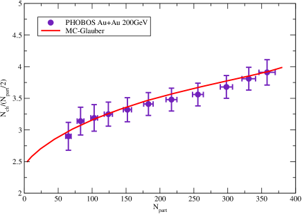
where is the particle multiplicity in a nucleon-nucleon collision at the same collision energy. The variable controls the balance between two components: participant scaling and binary collision scaling. With the value of , one may obtain a nice description of the centrality dependence of average charged particle multiplicity at midrapidity in Au+Au collisions at GeV Back:2002uc (see Fig. 1).
As is well known, the particle multiplicity in high energy collisions is fluctuating from one event to another. The distribution of particle multiplicities for a given rapidity range may be well described by a negative binomial (NB) distribution, Ansorge:1988kn ; Gans ; Adare:2008ns ,
| (7) |
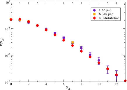
where is the mean of the distribution, and is related to the shape of the distribution. The variance is given by and the scaled invariance is defined as . With the values of and , one obtains a good description of the charge particle multiplicity measurements for both p+ collisions from UA5 Ansorge:1988kn , and p+p collisions from STAR Gans at midrapidity (see Fig. 2).
For high energy nucleus-nucleus collisions, we include particle multiplicity fluctuations by evaluating Eq.(II) on an event-by-event basis, with the distribution of given by Eq.(7). The balance factor of binary collision and participant scaling in Eq.(II) is implemented by randomly keeping only a fraction of particles from a binary collision, and a fraction of particles originating from a participating nucleon. In general the positions of particles might be sampled according to a smeared distribution around the positions of binary collisions or participant nucleons. Here we take the positions of particles as the same positions as binary collisions or participant nucleons. The Lorentz contraction in the longitudinal direction is taken into account by contracting the longitudinal position of each particle by a factor of for Au+Au collisions at GeV.
With the number of produced particles and their positions fixed, we also assign momenta to each particle. In this work, particle transverse momenta are sampled according to the following power law distribution,
| (8) |
where is the normalization constant, and and are taken as and . The azimuthal angle of the transverse momentum is uniformly distributed. Particle rapidities are taken to be uniformly distributed around mid-rapidity (When changing the rapidity range, we change both the mean and the parameter and keep the scaled variance of NB distribution fixed). Particles with large rapidities will be absent from the central rapidity region at later times and we neglect them in this work. With the above setup, we obtain the full phase distribution of the system at initial production time.
III Initial Geometry
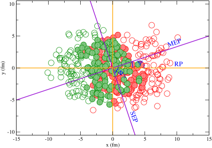
Before moving to the evolution of the system, we first investigate its geometrical properties at the production time. In a nucleus-nucleus collision, the reaction plane is defined by the beam direction () and the impact parameter direction (). The impact parameter direction and the third orthogonal direction () define the transverse plane (one typical collision event is shown Fig. 3). We call the plane defined by direction and direction the vertical plane. The geometry of the transverse plane is particularly interesting due to the fact that the elliptic flow is found in ideal hydrodynamics to be proportional to the initial eccentricity of the overlap region of the colliding nuclei, the determination of which plays an important role in the extraction of the transport coefficients of the produced fireball.
For averaged initial conditions, the geometry of the system can be studied directly in the above framework due to the coincidence of the vertical plane and the spatial event plane for (a rotation by of the participant plane if the participating nucleons are considered for the spatial distribution). With fluctuating initial conditions, the spatial event plane is tilted with respect to the reaction plane from one event to another. We call the angle between the spatial event plane and the reaction plane the spatial event plane angle . Note that this choice of the spatial event plane is convenient when generalizing to higher moments since the event plane angle distribution always has a maximum in the direction for all even moments whereas not always one of the minima is in the direction.
The final elliptic flow is defined with respect to a third plane, the momentum event plane that is reconstructed in experiments from the measured momentum distribution of the produced particles. Again in ideal hydrodynamics with smooth initial conditions this event plane coincides with the reaction plane, i.e., is rotated with respect to the spatial event plane by . This rotation ensures that the final has the same sign as the initial . If an event-by-event analysis with fluctuating initial conditions is applied, a strong correlation of the final momentum event plane to the initial spatial event plane still remains, but fluctuates around as has been shown in Holopainen:2010gz .
One may generalize the above concept for every harmonic moment, and define the spatial anisotropy parameters as follows. The first moment can always be made to vanish by shifting the coordinates to the center of mass (CM) frame of the system such that . Note throughout this paper represent averages over the phase space profile for a given event, except in the Appendix. Once the system is shifted to its CM frame, , all higher harmonic moments can be defined as:
| (9) |
where , and are polar coordinates in the transverse plane. The spatial event plane angle with respect to the reaction plane can be found through the following formula,
| (10) |
Note in our definition fluctuates from one event to another in the range of (), but it is equivalent to rotate such angle by . Once the event plane angle is found, the definition of the spatial anisotropy parameters may be reduced to .
The flow coefficients are defined as the -th Fourier moment of the particle momentum distribution with respect to each momentum event plane,
| (11) |
where is the azimuthal angle of particle momentum in the CM frame. Here we define the momentum event plane by a rotation angle with respect to the initial spatial event plane, . This rotation is just a convention generalized from the requirement that a positive initial eccentricity generates a positive value of final elliptic flow in ideal hydrodynamics with average initial conditions. Note our definition of the momentum event plane does not necessarily corresponds to the event plane that is reconstructed in experiments as just mentioned, but for our systematic study it provides an unambiguous basis to quantify the final state response to the initial state anisotropies.
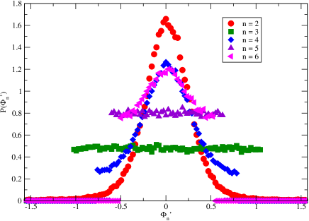
Since the event plane defined by Eq. (10) fluctuates around the vertical plane ( direction) for even moments, we may perform a transformation by evaluating Eq. (10) with . This corresponds to a rotation of the coordinate system by which ensures the distributions of all even peak at as shown in Fig. 4. In this plot, the impact parameter is taken to be fm for all events. While all even moments are strongly correlated with the reaction plane with one maximum along direction, all odd moments are uniformly distributed. This may be understood since the odd moments of spatial anisotropy purely originate from fluctuations while the even ones are combined effects of fluctuations and geometry. As a consequence, if one defines the spatial anisotropy parameters with respect to the pre-determined the reaction plane, the event-averaged vanishes for all odd moments, but not for even ones. We also observe that the distributions of even moments is wider for higher values of due to weaker correlations with respect to the reaction plane [in fact, what matters is the distribution of , as fluctuates within ].
We also investigate the centrality dependence of the above correlations in Fig. 5, where the widths of the distributions are plotted as a function of impact parameter . One can see that the widths all odd values of align with each other at as expected [for a uniform distribution from to , the variance is and we are plotting ]. Also due to symmetry in central collisions there is no correlation between the angle and direction for all values of . The anisotropy is purely from fluctuations, rendering uniform distributions also for even values of . As one moves to non-central collisions, geometry comes into play and may dominate over pure fluctuations, hence the widths of even distributions become smaller. For very peripheral collisions, the importance of the geometry diminishes due to the small size of the system, and even distributions become broader again. We also observe that even harmonic moments with higher values of have weaker dependence on centrality.
In Fig. 6, the first few spatial anisotropy parameters are plotted as a function of impact parameter ( is not shown). One may observe that all moments are of the same magnitude for typical non-central collisions. In central collisions, as pure fluctuations instead of geometry generate the anisotropy, higher moments acquire larger values due to larger fluctuations brought by the power in the definition of . Note that if the same weight, i.e., , is taken for every as in Ref. Alver:2010gr , all moments are the same in central collisions and is larger than all higher moments in non-central collisions (also note is non-zero if is used).
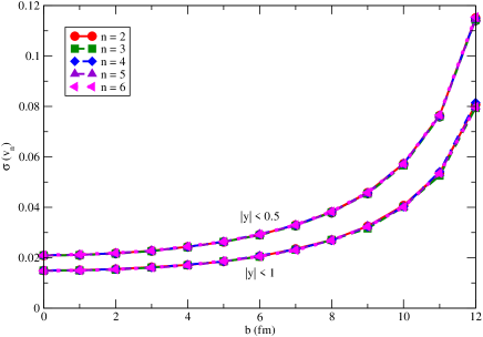
In our initial conditions, we may also calculate the momentum anisotropies as we have generated the full phase space distribution for the produced system. Since the initial particles are sampled with a symmetric azimuthal distribution, one obtains zero when averaging over events. In Fig. 7, the width of the initial distribution is plotted as a function of impact parameter . We find that the width increases as one moves from central collisions to non-central collisions due to the decrease in the number of particles in the produced system. In fact, the distribution is a Gaussian as a result of central limit theorem and its width is found to be for all values of , except for very peripheral collisions where the particle number is too small. The figure contains two sets of curves: the upper one is for all particles within a rapidity bin of and the lower one for . The curves are related by a factor of since the number of particles in the system is doubled via the doubling of the rapidity bin. The non-zero width of initial distribution helps to explain the wide distribution of the transformation matrix elements between initial and final as shown in Fig. 18. It serves as another source that contributes to final flow fluctuations in addition to initial state geometry fluctuations.
IV Pre-Equilibrium Phase
As to date, hydrodynamical simulations mostly use initial conditions calculated at the initial production time of the medium, and have neglected the influence of the pre-equlibrium time evolution of the colliding matter. In this sense, the spatial information inferred from comparing experimental measurements with hydrodynamical simulations is for the system at the starting time of the hydrodynamic evolution , not at the initial production time . However, the pre-equilibrium evolution may be important to include when considering the geometry fluctuations of the produced matter. Unlike the hydrodynamical evolution which directly translates the initial geometric anisotropies into the observed momentum anisotropies, the early pre-equilibrium expansion of the system will not only smear out the spatial fluctuations and change the local momentum distribution, but may also lead to correlations between odd and even moments. The inclusion of the pre-equilibrium evolution could be also important for studying the Hanbury-Brown–Twiss interferometri radii as it will generate some amount of early flow Jas:2007rw ; Broniowski:2008qk ; Broniowski:2008vp ; Pratt:2008qv .
To simulate the pre-equilibrium evolution, we solve the Boltzmann equation for the phase space distribution of the system,
| (12) |
Here, for simplicity massless particles are considered, . The free-streaming term will smear out the spatial fluctuations and change the local momentum distribution due to pure fluctuations. The collision term is important for studying the details of the thermalization of the system, a complex issue which has not been fully understood yet. In this work, we focus on the effect of the pre-equilibrium expansion on the system geometry and only include the free-streaming term by setting . Such a treatment is important for our study as the flow built up by hydrodynamical evolution is mostly driven by spatial anisotropy. The consideration of the collision term will remain for a future project. The Boltzmann equation containing only the free-steaming term can be solved analytically, with the streaming solution given by , where is the initial starting time of the evolution.
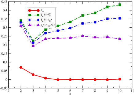
The effect of free-streaming on the spatial anisotropies during the early expansion is shown in Fig. 8, where the ratios of anisotropy parameters evaluated at fm/c to those at the production time are shown as a function of centrality. As expected, the expansion of the matter due to free-streaming smears out the spatial fluctuations: all the spatial anisotropy parameters become smaller. This diminishing effect is more pronounced in non-central collisions due to the smaller size of the system. We also observe that higher moments get more diminished than lower moments.
We further explore the time evolution of the above smearing effect due to free-streaming as shown in Fig. 9, where at an impact parameter of fm is plotted as a function of time. We observe that the anisotropy parameters decrease rather fast for the first fm/c and then slowly saturate. The observed reduction of the hints at the importance of including the pre-equilibrium expansion when studying the initial state geometry fluctuations for hydrodynamical simulations. The relative size of the different coefficients even depends on the duration of the pre-equilibrium expansion and the relative size of the resulting flow coefficients might be used to constrain this initial evolution.
As we just mentioned, there are two separate effects due to the pre-equilibrium evolution: the pure drift effect due to the system expansion which tends to diminish all moments, and the correlations between odd and event moments which is absent in the later hydrodynamical evolution. The mixing effect between odd and event moments can be clearly seen when one explicitly performs a multipole-expansion analysis for the Boltzmann equation. To start, we choose spherical polar coordinates for both coordinate space and momentum space . To make the analysis dimensionless, we define and , where and are two dimensional quantities (being constants or varying with time). Then we expand the phase space distribution as
| (13) |
In the above expression,
| (14) |
where is the spherical Bessel function with the th root of function , the -th order Laguerre function (Here we choose ) and the spherical harmonics. The expansion coefficients are determined from the phase space distribution by
| (15) |
The spatial anisotropy parameters are related to the expansion coefficients , by
| (16) |
where
| (17) |
The normalization factor represents the total number of particles in the system, which is given by
| (18) |
Note for and which appear in the definition of , there will be an extra factor in the integral .
Within the above multipole expansion analysis, the Boltzmann equation becomes,
| (19) |
where
| (20) |
Note the indices in in , which do not allow us to perform the integral using orthogonal relations. are the Clebsch-Gordan coefficients for adding two angular momenta . More details of the derivation are presented in the Appendix.
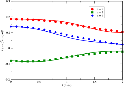
From the above equations, one immediately sees the mixing between odd and even moments both for spatial part () and momentum part () due to the free-streaming of particles. We also check the above expression by comparing numerically with the result from directly solving free-streaming part of Boltzmann equation. This is shown in Fig. 10, where we plot the time evolution of for one typical event with impact parameter fm and see that the two results nicely agree with each other.
In order to further separate the correlation effect from the pure drifting effect during the pre-equilibrium expansion, we perform the following analysis. We relate the spatial anisotropies at two different times by a transformation matrix,
| (27) |
Here we only consider the second and third moments – the inclusion of higher order moments is straightforward and is expected to give only small contributions which we neglected in the current analysis. The diagonal elements of the transformation matrix quantify the pure drifting effect and the off-diagonal elements represent the effect of the mixing between the second and third moments. We obtain the distribution of the transformation matrix elements by pairing two linear independent events from a large set of events.
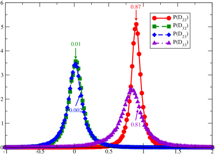
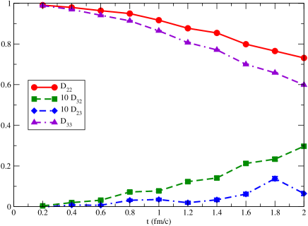
In Fig. 11, we show the probability distribution of four elements of the above transformation matrix, with the pre-equilibrium expansion time taken to be fm/c. The numbers in the figure represent the mean of each distribution (to which the arrows point). The impact parameter is taken to be fm for all events in this plot. One clearly observes the smearing effect from the free streaming when one looks at the distributions of the two diagonal elements. The pure drifting effect is more pronounced for the third anisotropy parameter () than for the second one (), consistent with the above results. The two off-diagonal elements are close to zero implying weak correlations between and originating from the free-streaming of the system. We further investigate the time evolution of these matrix elements up to fm/c in Fig. 12. Both the drifting effect and the mixing of even and odd moments tend to increase with time as the system expands.
V Hydrodynamical Evolution
In the previous sections, we have presented the initial conditions of the system at production time and simulated the pre-equilibrium evolution by utilizing the free-streaming approximation. As we have not included interaction among the produced particles, the system is still highly non-thermal. Up to know, little knowledge has been attained about the details of the thermalization mechanisms in relativistic heavy-ion collisions. In this work, we follow the common practice to assume a sudden thermalization of the system at and start the hydrodynamical evolution with the initial conditions obtained above (including the free streaming evolution from to ). We first calculate the energy-momentum tensor from the full phase space distribution ,
| (28) |
For our discretized phase space distribution , the momentum integration turns into sums over all particles. The discretized spatial part is smeared with a Gaussian function in order to ensure a sufficiently continuous distribution necessary for the hydrodynamic simulation,
| (29) |
where the widths and characterize the granularity of the system in the transverse and longitudinal directions. Physically, this procedure can be interpreted as thermal smearing of the system which should have occurred prior to thermalization at . In general the choice of these width parameters depends on the duration of the pre-equilibrium phase and the thermalization time at which one starts the hydrodynamic evolution. Different choices of the smearing width will affect the local density of the system, and thus influence the spatial anisotropy parameters.
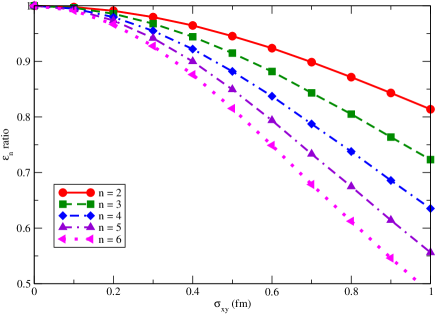
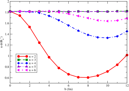
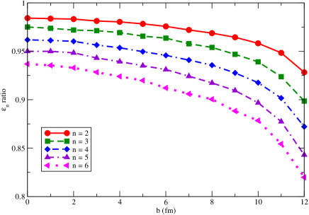
The effect of the Gaussian smearing on the spatial anisotropy is shown in Fig 13, where the ratio of anisotropy parameters with smearing to these without smearing is shown as a function of transverse smearing width . As we are studying the spatial anisotropy in the transverse plane, the smearing of the longitudinal direction should be irrelevant and we fix it to be fm for our study. The impact parameter is taken to be fm for all calculations shown in this figure. As expected, the spatial anisotropies are reduced as one increases the width of the transverse Gaussian function. Similar to pre-equilibrium evolution shown before, such smearing effect is more prominent for higher moments than for lower moments. Combining both effects (pre-equilibrium evolution and Gaussian smearing), for typical non-central collisions may be reduced by about for a Gaussian width of fm and a typical pre-equilibrium evolution time of fm; a factor of larger effect is observed for for .
In the above construction of the energy-momentum tensor, the initial conditions at production time are fitted to the final state particle multiplicity distribution at midrapidity (see Fig. 1 and 2). Therefore, the energy density of the system at the thermalization time is underestimated, due to the longitudinal (and transverse) expansion during the hydrodynamical evolution. This effect can be estimated to be about a factor of by directly comparing our calculation to the final average charged particle multiplicity in central Au+Au collisions at GeV. We have not tuned our parameters to match the final state particle spectra as we are here not aiming at providing a comprehensive quantitative description of the time-evolution of a heavy-ion collision, but rather at a targeted study of initial state fluctuations and how these initial spatial anisotropies propagate through the fireball history and translate themselves into collective flow in the final state.
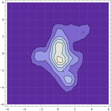
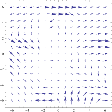
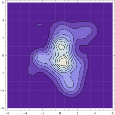
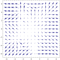
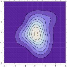
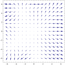
In Fig. 14, we show the a few snapshots of the energy momentum tensor components in the transverse plane (the horizontal and vertical axes are and axes in unit of fm) for one typical event with an impact parameter fm. To illustrate the effects of the pre-equilibrium evolution and Gaussian smearing of discretized space distribution, we plot three different sets of pre-equilibrium time and Gaussian smearing width: the upper for and fm, the middle for fm/c and fm, and the lower for fm/c and fm. On the left we show the distribution of and on the right the flow vector , with the arrows representing the directions and the lengths of arrows for the relative magnitudes of the vectors (within each plot). Comparing the left and middle panels, one can clearly see that pre-equilibrium evolution makes the system larger (thus the energy density becomes smaller) and generates some amount of radial flow. The effect of Gaussian smearing can be seen by comparing the middle and right panels: both the energy density and the flow velocity smoothen out significantly when one increases the Gaussian width.
After obtaining the energy momentum tensor as described above, we directly start the hydrodynamical evolution with the assumption of a sudden thermalization,
| (30) |
Here an ideal hydrodynamical evolution code Rischke:1995ir ; Rischke:1995mt is utilized for our study with a lattice equation of state Steinheimer:2009nn ; Steinheimer:2009hd for the hot and dense matter created in Au+Au collision at GeV. Particle production at the end of the hydrodynamic evolution when the matter is diluted in the late stage is treated as a gradual freeze-out on an approximated iso-eigentime hyper-surface according to the Cooper-Frye prescription Li:2008qm ; Steinheimer:2009nn . For simplicity, we have not taken into account the hadronic rescattering in the dilute hadron gas and the resonance decays, since they should not have much influence on the results for the charged particle flow coefficients as has been shown in Petersen:2010md .
VI From Initial Geometry Fluctuations to Final Flow
The above event-by-event setup of the system evolution from initial production time to the freeze-out of the final state should include all ingredients that are necessary for the study of the build-up of collective flow during the hydrodynamical evolution. For the following results, we use the produced charged particles with transverse momenta GeV/c and peudorapidity .
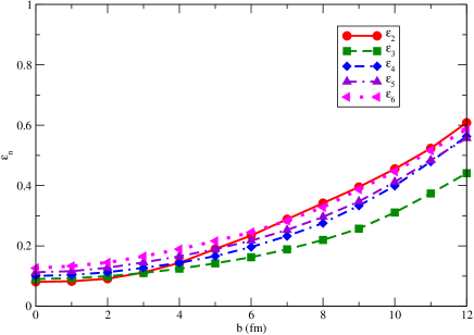
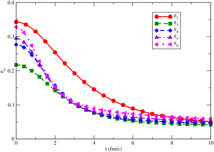
In Fig. 15, we show the first few flow coefficients for final state particles together with three different spatial anisotropies evaluated at the production time, at before and after Gaussian smearing. In this figure, the impact parameter is randomly sampled in the fm bin according to the probability distribution , the pre-equilibrium evolution time is set as fm/c prior to the hydrodynamical evolution, and the Gaussian widths for smearing the discretized initial conditions are taken to be fm. One can see that all flow coefficients with greater than are negligible and only the first few (, 3, 4) survive after the hydrodynamical evolution. We may conclude that the analysis of flow coefficients allows only for the extraction of the first few spatial anisotropy parameters , but may not provide sufficient information to recover the full initial geometry in terms of all of its higher order harmonics. In order to achieve this, one needs additional observables with an increased sensitivity to the higher order spatial anisotropy parameters. We also note that the spatial asymmetry obtained from comparing flow measurements to a hydrodynamical simulation only applies to the spatial characteristics of matter at the starting time of hydrodynamical evolution . In order to obtain the geometry at the initial production time , one needs to account for the dynamics of the pre-equilibrium phase – in our analysis this would be the smearing effects during the initial free streaming of the particles and the smoothing of the discretized initial conditions as shown in the figure.
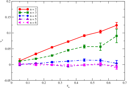
In order to study the response of flow build-up to the initial geometry, Fig. 16 shows the first few flow coefficients as a function of the corresponding spatial anisotropy parameter evaluated at the production time. As expected, the hydrodynamical evolution translates spatial anisotropies into momentum anisotropies, resulting in an essentially linear relation between and . We also observe that the curves have smaller slopes for higher moments and become more or less flat when is greater than . This implies that higher flow coefficients show weaker response to the corresponding geometrical harmonic moments due to larger diminishing effect originating from the combination of pre-equilibrium evolution, Gaussian smearing of the discretized spatial distribution, and the hydrodynamical evolution, all of which tend to lead to a larger suppression for the higher moments.
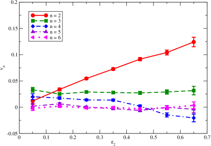
We also explore the correlations between different harmonics moments. As an illustration, we plot the first few flow coefficients as a function of the second spatial anisotropy parameter . On can see that except for versus , all other curves are essentially flat due to the combined effect of the small correlations between odd and even moments and the reduced effect on higher moments from the pre-equilibrium and hydrodynamical evolution.
In order to separate the pure smearing effect from the mixing effect between different moments, we perform an analysis similar to that for the pre-equilibrium evolution. On may define the transformation matrix between the initial spatial anisotropy and the final flow coefficients as
| (31) |
where characterizes the strength of the coupling between initial and final . The diagonal elements of the transformation matrix quantify the response of to and the off-diagonal elements represent the effect of the mixing response between different moments and . Here again we only consider the second and third moment,
| (38) |
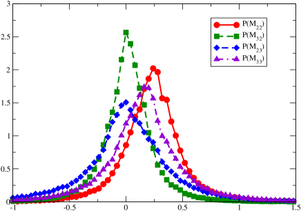
The extension of this ansatz to include higher order moments is straightforward and expected to only give small contributions to the dominant moments . The distribution of the transformation matrix elements is obtained by solving two linear independent equations which correspond to a pair of linear independent events chosen from a large set of events.
In Fig. 18, we show the probability distribution of the four elements of the transformation matrix between final , and initial , . We find that for the two diagonal elements is larger than , implying stronger response of to than to as expected from Fig. 16. The two off-diagonal elements and again are very small, implying a weak response of to during the hydrodynamical evolution. Another interesting feature is the wide distribution of the transformation matrix which encodes the fluctuations of final flow coefficients. We note two initial state effects that contribute to such wide distribution: initial geometry fluctuations and initial fluctuations (see Fig. 7). If one wants to extract information about the initial collision geometry from the measured flow anisotropies, it is important to separate the two sources of fluctuations in the transformation matrix. Experimentally, this could be achieved by measuring the rapidity correlations of the final flow coefficients since the initial state geometry fluctuations are expected to be long-range in rapidity, while initial state flow fluctuations should decrease when one makes the rapidity window wider.
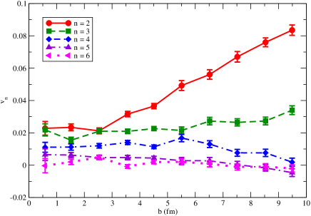
Finally, we explore the centrality dependence of the final state flow coefficients as shown in Fig. 19. The splitting of is clearly seen for all centralities: the lower are larger than higher , at least for the first few (when , are so small that it is difficult to resolve their splitting). For the most central collisions, our statistics is not sufficient to distinguish between different curves, but one would expect the same ordering, even though the splitting might be smaller. This is due to pure fluctuations being the only source of spatial anisotropies for both odd and event moments in central collisions, and the smearing effect in the subsequent pre-equilibrium evolution is more prominent for higher moments, thus leading to less flow builtup for higher order during the hydrodynamical evolution. One observes different centrality dependencies for different : the lowest have the strongest centrality dependence.
VII Summary
We have presented a systematic study of initial collision geometry fluctuations and have investigated how they evolve throughout the whole history of the collision and finally translate into measurable momentum anisotropies of the produced hadrons. Our initial conditions at production time are obtained via a Monte Carlo Glauber model with the inclusion of nucleon position fluctuations, plus additional fluctuations stemming from individual nucleon-nucleon collisions. In addition we make an ansatz for the initial transverse momentum distribution of the produced particles which is important for the treatment of the pre-equilibrium phase of the collision. We evolve our full phase space distribution using a Boltzmann equation and approximate the pre-equilibrium evolution by treating all particles as free streaming. A sudden thermalization of our initial conditions is enforced for the subsequent hydrodynamic evolution of the thermalized system, which is performed using three-dimensional relativistic ideal hydrodynamics.
Our analysis shows that though all initial spatial anisotropy parameters are of the same magnitude, only the first few flow coefficients for the momentum anisotropy of final state hadrons actually survive after hydrodynamical evolution. We also quantitatively investigate the mixing between odd and even harmonic moments during the pre-equilibrium evolution and its effect on the evolution of the system asymmetry is found to be small. The anisotropy of the matter is found to be affected by the pre-equilibrium evolution and by the smoothing of the discretized initial conditions necessary for the hydrodynamical evolution (which can be seen as equivalent to thermal smearing expected to occur during thermalization), both of which tend to smear out the spatial anisotropies. The hydrodynamical evolution leads to an additional dampening of the flow response to the initial spatial anisotropies, particularly for the higher order moments. This makes it difficult to recover the full geometry of the initial state from measuring high order flow coefficients which have the ability to provide additional information on the transport properties of the produced matter. We also observe the contribution of initial state flow fluctuations to final flow fluctuations, which could be separated by rapidity correlation measurements for a better understanding of initial state geometry fluctuations.
In summary, we have conducted an event-by-event study of the time evolution of the multipole moments of the collision geometry in a relativistic heavy-ion collision. Our study sheds light on how these multipole moments relate to measurable collective flow coefficients of the hadronic final state and how the collision dynamics, both in the pre-equilibrium and in the hydrodynamic evolution phase, affect the correlation between the initial spatial anisotropies and the final momentum space anisotropies. It allows for improved constraints on the determination of various transport properties of the QCD medium, which commonly are extracted by analyzing the observed momentum anisotropy of the final particles and are very sensitive to the proper description of initial spatial anisotropies. Our current work can be improved in many directions. Here, we have only focused on the qualitative study of the propagation of the initial state geometry fluctuations; a more quantitative study including a comparison with experimental measurements would be desirable. The pre-equilibrium phase has been approximated by free-streaming of particles; we fully expect that the inclusion of a realistic collision term in the Boltzmann equation would provide more sophisticated initial conditions for the hydrodynamic evolution. We have performed our calculations using ideal hydrodynamics; improving these with the use of viscous hydrodynamics should help to separate viscosity dominated effects from non-viscous effects on the evolution of the geometry fluctuations. All these tasks we leave to future investigations.
VIII Acknowledgments
We thank Dirk Rischke for providing the three-dimensional relativistic hydrodynamics code. This work was supported in part by U.S. department of Energy grant DE-FG02-05ER41367. Some of the calculations were performed using resources provided by the Open Science Grid, which is supported by the National Science Foundation and the U.S. Department of Energy. H.P. acknowledges a Feodor Lynen fellowship of the Alexander von Humboldt foundation.
Appendix A Multipole Expansion
In this appendix, we present more details of the multipole expansion of the left hand side of the Boltzmann equation. The first term is straightforward,
| (39) |
Note and . If and/or vary with time, then one needs to include additional terms which we do not elaborate in details. To obtain the evolution equation for the expansion coefficients , we define the following shorthand to project out the expansion coefficients from any function ,
| (40) |
Performing such projection for the first term, we obtain
| (41) |
The second term involves the gradient of a function of times a spherical harmonics. We note the following gradient formula,
| (42) |
Here represent Clebsch-Gordan coefficients for adding two angular momenta . The spherical basis vectors are defined as
| (43) |
The use of spherical basis vectors is convenient as three components of a vector are directly related to spherical harmonics ,
| (44) |
The gradient formula Eq. (A) can be further simplified if one has spherical Bessel function, , with the help of the following recurrence relations
| (45) |
Applying to the first and second terms in Eq. (A), one has for our case
| (46) |
where we have combined two terms together into a compact form. The second term becomes
| (47) |
Following the same procedure as done for the first term, we project out the expansion coefficients for the second term,
| (48) |
The integrals and can be done using orthogonal relations for spherical harmonics and Laguerre function. The integral involves the product of three spherical harmonics, which can performed with the help of the following relation,
| (49) |
Note that the above Clebsch-Gordan coefficients are non-zero only when and are even numbers. This implies that and . The final result for the second term is,
where has been defined in Eq. (IV). Combining with the first term, we finish the multipole expansion of the left hand side in Boltzmann equation.
References
- (1) P. F. Kolb, J. Sollfrank, and U. W. Heinz, Phys. Rev. C62, 054909 (2000), arXiv:hep-ph/0006129.
- (2) D. Teaney, J. Lauret, and E. V. Shuryak, Phys. Rev. Lett. 86, 4783 (2001), arXiv:nucl-th/0011058.
- (3) P. Huovinen, P. F. Kolb, U. W. Heinz, P. V. Ruuskanen, and S. A. Voloshin, Phys. Lett. B503, 58 (2001), arXiv:hep-ph/0101136.
- (4) T. Hirano and K. Tsuda, Phys. Rev. C66, 054905 (2002), arXiv:nucl-th/0205043.
- (5) P. Huovinen, Nucl. Phys. A761, 296 (2005), arXiv:nucl-th/0505036.
- (6) C. Nonaka and S. A. Bass, Phys. Rev. C75, 014902 (2007), arXiv:nucl-th/0607018.
- (7) B. Schenke, S. Jeon, and C. Gale, Phys. Rev. C82, 014903 (2010), arXiv:1004.1408.
- (8) H. Niemi, K. J. Eskola, and P. V. Ruuskanen, Phys. Rev. C79, 024903 (2009), arXiv:0806.1116.
- (9) J.-Y. Ollitrault, Phys. Rev. D46, 229 (1992).
- (10) STAR, J. Adams et al., Phys. Rev. Lett. 92, 062301 (2004), arXiv:nucl-ex/0310029.
- (11) D. Teaney, Phys. Rev. C68, 034913 (2003), arXiv:nucl-th/0301099.
- (12) P. Romatschke and U. Romatschke, Phys. Rev. Lett. 99, 172301 (2007), arXiv:0706.1522.
- (13) H. Song and U. W. Heinz, Phys. Lett. B658, 279 (2008), arXiv:0709.0742.
- (14) K. Dusling and D. Teaney, Phys. Rev. C77, 034905 (2008), arXiv:0710.5932.
- (15) M. Luzum and P. Romatschke, Phys. Rev. C78, 034915 (2008), arXiv:0804.4015.
- (16) Z. Xu, C. Greiner, and H. Stocker, Phys. Rev. Lett. 101, 082302 (2008), arXiv:0711.0961.
- (17) H.-J. Drescher, A. Dumitru, C. Gombeaud, and J.-Y. Ollitrault, Phys. Rev. C76, 024905 (2007), arXiv:0704.3553.
- (18) H. Song and U. W. Heinz, J. Phys. G36, 064033 (2009), arXiv:0812.4274.
- (19) J. L. Nagle, P. Steinberg, and W. A. Zajc, Phys. Rev. C81, 024901 (2010), arXiv:0908.3684.
- (20) P. Kovtun, D. T. Son, and A. O. Starinets, Phys. Rev. Lett. 94, 111601 (2005), arXiv:hep-th/0405231.
- (21) N. Demir and S. A. Bass, Phys. Rev. Lett. 102, 172302 (2009), arXiv:0812.2422.
- (22) H. Song and U. W. Heinz, Phys. Rev. C81, 024905 (2010), arXiv:0909.1549.
- (23) T. Hirano, U. W. Heinz, D. Kharzeev, R. Lacey, and Y. Nara, Phys. Lett. B636, 299 (2006), arXiv:nucl-th/0511046.
- (24) M. Miller and R. Snellings, (2003), arXiv:nucl-ex/0312008.
- (25) W. Broniowski, P. Bozek, and M. Rybczynski, Phys. Rev. C76, 054905 (2007), arXiv:0706.4266.
- (26) B. Alver et al., Phys. Rev. C77, 014906 (2008), arXiv:0711.3724.
- (27) T. Hirano and Y. Nara, Nucl. Phys. A830, 191c (2009), arXiv:0907.2966.
- (28) P. Staig and E. Shuryak, (2010), arXiv:1008.3139.
- (29) A. Mocsy and P. Sorensen, (2010), arXiv:1008.3381.
- (30) R. J. Glauber and G. Matthiae, Nucl. Phys. B21, 135 (1970).
- (31) M. L. Miller, K. Reygers, S. J. Sanders, and P. Steinberg, Ann. Rev. Nucl. Part. Sci. 57, 205 (2007), arXiv:nucl-ex/0701025.
- (32) H. Petersen and M. Bleicher, Phys. Rev. C81, 044906 (2010), arXiv:1002.1003.
- (33) H. Holopainen, H. Niemi, and K. J. Eskola, (2010), arXiv:1007.0368.
- (34) H. Petersen, G.-Y. Qin, S. A. Bass, and B. Muller, (2010), arXiv:1008.0625.
- (35) B. Alver and G. Roland, Phys. Rev. C81, 054905 (2010), arXiv:1003.0194.
- (36) B. H. Alver, C. Gombeaud, M. Luzum, and J.-Y. Ollitrault, (2010), arXiv:1007.5469.
- (37) the STAR, B. I. Abelev et al., Phys. Rev. C75, 054906 (2007), arXiv:nucl-ex/0701010.
- (38) PHENIX, A. Adare et al., Phys. Rev. Lett. 105, 062301 (2010), arXiv:1003.5586.
- (39) C. Gombeaud and J.-Y. Ollitrault, Phys. Rev. C81, 014901 (2010), arXiv:0907.4664.
- (40) M. Luzum, C. Gombeaud, and J.-Y. Ollitrault, Phys. Rev. C81, 054910 (2010), arXiv:1004.2024.
- (41) D. H. Rischke, S. Bernard, and J. A. Maruhn, Nucl. Phys. A595, 346 (1995), arXiv:nucl-th/9504018.
- (42) D. H. Rischke, Y. Pursun, and J. A. Maruhn, Nucl. Phys. A595, 383 (1995), arXiv:nucl-th/9504021.
- (43) D. Kharzeev and M. Nardi, Phys. Lett. B507, 121 (2001), arXiv:nucl-th/0012025.
- (44) PHOBOS, B. B. Back et al., Phys. Rev. C65, 061901 (2002), arXiv:nucl-ex/0201005.
- (45) UA5, R. E. Ansorge et al., Z. Phys. C43, 357 (1989).
- (46) J. Gans, Ph.D. thesis (2004).
- (47) PHENIX, A. Adare et al., Phys. Rev. C78, 044902 (2008), arXiv:0805.1521.
- (48) S. Pratt, Phys. Rev. Lett. 102, 232301 (2009), arXiv:0811.3363.
- (49) W. Broniowski, M. Chojnacki, W. Florkowski, and A. Kisiel, Phys. Rev. Lett. 101, 022301 (2008), arXiv:0801.4361.
- (50) W. Jas and S. Mrowczynski, Phys. Rev. C76, 044905 (2007), arXiv:0706.2273.
- (51) W. Broniowski, W. Florkowski, M. Chojnacki, and A. Kisiel, Phys. Rev. C80, 034902 (2009), arXiv:0812.3393.
- (52) J. Steinheimer et al., Phys. Rev. C81 (2010), arXiv:0905.3099.
- (53) J. Steinheimer, S. Schramm, and H. Stocker, (2009), arXiv:0909.4421.
- (54) Q.-f. Li, J. Steinheimer, H. Petersen, M. Bleicher, and H. Stocker, Phys. Lett. B674, 111 (2009), arXiv:0812.0375.