Quantum Interference between a Single-Photon Fock State and a Coherent State

Abstract

We derive analytical expressions for the single mode quantum field state at the individual output ports of a beam splitter when a single-photon Fock state and a coherent state are incident on the input ports. The output states turn out to be a statistical mixture between a displaced Fock state and a coherent state. Consequently we are able to find an analytical expression for the corresponding Wigner function. Because of the generality of our calculations the obtained results are valid for all passive and lossless optical four port devices. We show further how the results can be adapted to the case of the Mach-Zehnder interferometer. In addition we consider the case for which the single-photon Fock state is replaced with a general input state: a coherent input state displaces each general quantum state at the output port of a beam splitter with the displacement parameter being the amplitude of the coherent state.

PACS. 42.50.Dv
Key words: coherent state, displaced Fock state, Mach-Zehnder, entanglement, quantum interference

I Introduction

Quantum optics is an exciting field, in which many fundamental experiments, revealing the peculiarities of quantum mechanics, have been conducted. The advantage of optical experiments, compared with other fundamental experiments, is their simplicity. Quantum optics has been one of the main vehicles in the development of quantum information technologies and in particular of quantum cryptography quantumcryptography ; continuousvariableQKD ; Chuang ; Gisin and optical quantum computing quantcomputing1 ; quantcomputing2 ; Chuang . The most widely used quantum states in this respect are coherent states and Fock states M&W . Important basic building blocks in quantum optics are beam splitters and Mach-Zehnder interferometers, which are passive and lossless four port devices BS2 ; Yurke ; Knight . Many cases of interference between vacuum, Fock states and coherent states have already been theoretically studied Knight . A famous example is the so called Hong-Ou-Mandel effect HongOuMandel where two single-photon Fock states arrive simultaneously at each input port of a balanced beam splitter. In this case there are no coincident photons at the output ports. On the other hand interference between a fluorescent photon and a classical field has been investigated HOM88 where the photon is created from a coherently excited atom going through its Rabi cycle of oscillation. This results in a time dependence of the interferometric fringe visibility as a function of the atomic Rabi frequency Bali93 .

Without going into details of the time-dependent photon generation a somewhat simpler but nevertheless important problem arises when we consider the interference between a true single-photon Fock $|1\rangle$ state and a coherent state $|\alpha\rangle$. Based on an experiment in 2002 a displaced Fock state has been synthesized to a good approximation by overlapping a single-photon Fock state with a strong coherent pulse on a highly reflective beam splitter Lvovsky . To the best of our knowledge an exact analytical expression for the evolving quantum state in this experiment has not been published so that the reconstructed state (Wigner function) of the beam splitter output could be compared with the theory.

In this work we calculate analytically the output of a beam splitter (BS) in the case of a single-photon Fock state $\ket{1}$ and a coherent state $\ket{\alpha}$ impinging respectively on its two input ports. In particular we derive an exact expression for the quantum state of the separate beam splitter output ports. Because of the generality of our calculations, the results we obtain are not restricted to the beam splitter, but are valid for all passive and lossless optical four port devices. In addition we consider the case for which the single-photon Fock state is replaced with a general input state. We show that a coherent input state displaces the quantum state at the output port of a beam splitter in phase space, whereby the displacement parameter is the amplitude of the coherent state. In the second part of this paper we show how the results can be adapted to the case of a Mach-Zehnder interferometer (MZI). Additionally, the mean photon numbers at the output ports of the MZI are determined. These results serve as a first step of investigating more complex systems that might find application in optical quantum computation.

The intention of this article is to present the matter in a concise and didactic way.

Figure 1: Beam Splitter (BS) with a single-photon Fock state $\ket{1}_{0}$ and a coherent state $\ket{\alpha}_{1}$ incident on its input ports.

II Interference at a beam splitter

We consider a general beam splitter with complex reflection coefficients $r$ and $r^{\prime}$ and transmission coefficients $t$ and $t^{\prime}$. The phase relation between the coefficients depends on the construction of the beam splitter BSHamilton . In the Heisenberg picture the annihilation operators $\hat{a}$ of the incident fields transform as Knight

$$\left(\begin{array}[c]{cc}\hat{a}_{2}\\ \hat{a}_{3}\end{array}\right)\,\,\,=\left(\begin{array}[c]{cc}t^{\prime}&r\\ r^{\prime}&t\end{array}\right)\left(\begin{array}[c]{cc}\hat{a}_{0}\\ \hat{a}_{1}\end{array}\right)=B\left(\begin{array}[c]{cc}\hat{a}_{0}\\ \hat{a}_{1}\end{array}\right),$$ (9)

where the indices indicate the corresponding ports (modes). The unitary scattering matrix $B$ must satisfy - for lossless devices - the so called reciprocity relations due to Stokes Stokes

$$\left|r^{\prime}\right|=\left|r\right|,\quad\left|t\right|=\left|t^{\prime}\right|,\quad\left|r\right|^{2}+\left|t\right|^{2}=1\,\,\,,\,\,\,r^{*}t^{\prime}+r^{\prime}t^{*}=0.$$ (10)

II.1 Input: Fock state and Coherent state

In our setup (see Fig. 1) the incident field states are a single-photon Fock state $\ket{1}_{0}$ and a coherent state $\ket{\alpha}_{1}$ which can be written as the following product state:

$$\ket{1}_{0}\ket{\alpha}_{1}=\hat{D}_{1}(\alpha)\hat{a}_{0}^{\dagger}\ket{0}_{0}\ket{0}_{1}=e^{\alpha\hat{a}_{1}^{\dagger}-\alpha^{*}\hat{a}_{1}}\hat{a}_{0}^{\dagger}\ket{0}_{0}\ket{0}_{1},$$ (11)

where $\hat{a}^{\dagger}_{0}$ is the creation operator and $\hat{D}_{1}(\alpha)$ is the unitary displacement operator.

From Eq. (9) together with Eq. (10) we easily obtain the following relations:

$$\hat{a}_{0}^{\dagger}=t^{\prime}\hat{a}_{2}^{\dagger}+r^{\prime}\hat{a}_{3}^{\dagger}\,\,\mbox{and}\,\,\hat{a}_{1}^{\dagger}=r\hat{a}_{2}^{\dagger}+t\hat{a}_{3}^{\dagger}.$$ (12)

Obviously two vacuum states at the input ports of the beam splitter transform into vacuum states at the output ports: $\ket{0}_{0}\ket{0}_{1}\xrightarrow{BS}\ket{0}_{2}\ket{0}_{3}$. We use the Baker-Campbell-Hausdorff formula Knight and Eq. (12) to see how the input state Eq. (11) transforms into the corresponding output state under the action of the beam splitter:

$$\ket{1}_{0}\ket{\alpha}_{1}\xrightarrow{BS}e^{\alpha(r\hat{a}_{2}^{\dagger}+t\hat{a}_{3}^{\dagger})-\alpha^{*}(r^{*}\hat{a}_{2}+t^{*}\hat{a}_{3})}(t^{\prime}\hat{a}_{2}^{\dagger}+r^{\prime}\hat{a}_{3}^{\dagger})\ket{0}_{2}\ket{0}_{3}$$

$$=\hat{D}_{2}(r\alpha)\hat{D}_{3}(t\alpha)(t^{\prime}\hat{a}_{2}^{\dagger}+r^{\prime}\hat{a}_{3}^{\dagger})\ket{0}_{2}\ket{0}_{3}.$$ (13)

The density operator for the output state, Eq. (13), reads

$$\hat{\rho}_{23} =\hat{D}_{2}(r\alpha)\hat{D}_{3}(t\alpha)\hat{\tilde{\rho}}_{23}\hat{D}_{3}^{\dagger}(t\alpha)\hat{D}_{2}^{\dagger}(r\alpha),$$ (14)

where

$$\hat{\tilde{\rho}}_{23}=(t^{\prime}\hat{a}_{2}^{\dagger}+r^{\prime}\hat{a}_{3}^{\dagger})\ket{0}_{2}\ket{0}_{3}\bra{0}_{3}\bra{0}_{2}(t^{\prime*}\hat{a}_{2}+r^{\prime*}\hat{a}_{3}).$$ (15)

In fact $\hat{\tilde{\rho}}_{23}$ would be the density operator of the beam splitter output with vacuum instead of the coherent input state. The two output modes (2 and 3) are in an entangled state. If we consider only output mode 3 we have to find the reduced density matrix by taking the partial trace over output 2, i.e.

$$\hat{\rho}_{3} =\operatorname{Tr}_{2}(\hat{\rho}_{23})=\hat{D}_{3}(t\alpha)\operatorname{Tr}_{2}\left(\hat{D}_{2}(r\alpha)\hat{\tilde{\rho}}_{23}\hat{D}^{\dagger}_{2}(r\alpha)\right)\hat{D}^{\dagger}_{3}(t\alpha)$$

$$=\hat{D}_{3}(t\alpha)\operatorname{Tr}_{2}\left(\hat{D}^{\dagger}_{2}(r\alpha)\hat{D}_{2}(r\alpha)\hat{\tilde{\rho}}_{23}\right)\hat{D}^{\dagger}_{3}(t\alpha)$$

$$=\hat{D}_{3}(t\alpha)\sum_{n=0}^{\infty}\left<n\right|_{2}\hat{\tilde{\rho}}_{23}\left|n\right>_{2}\hat{D}^{\dagger}_{3}(t\alpha).$$ (16)

The operators $D_{3}(t\alpha)$ and $D_{3}^{\dagger}(t\alpha)$ are not effected by the trace over mode 2, therefore we can put them outside the trace. Further, in the second and third line of the last equation we made use of the rule that the trace is invariant under cyclic permutations, $\mbox{Tr}(ABC)=\mbox{Tr}(CAB)$, and the unity relation $\hat{D}^{\dagger}(\alpha)\hat{D}(\alpha)=1$. Inserting $\hat{\tilde{\rho}}_{23}$ into the last equation we get with some basic boson algebra

$$\hat{\rho}_{3}=\left|t^{\prime}\right|^{2}\ket{t\alpha}_{3}\bra{t\alpha}_{3}+\left|r^{\prime}\right|^{2}\hat{D}_{3}(t\alpha)\ket{1}_{3}\bra{1}_{3}\hat{D}_{3}^{\dagger}(t\alpha).$$ (17)

The result is a mixed state which is a convex combination of two pure identically displaced states: a coherent state (displaced vacuum) and a displaced Fock state Oliv , where the displacement and the share of each pure state depends on the reflectivity and the transmittivity of the beam splitter. For the other output port we get the analogous result

$$\hat{\rho}_{2}=\left|r\right|^{2}\ket{r\alpha}_{2}\bra{r\alpha}_{2}+\left|t\right|^{2}\hat{D}_{2}(r\alpha)\ket{1}_{2}\bra{1}_{2}\hat{D}_{2}^{\dagger}(r\alpha).$$ (18)

II.2 Wigner function

With the simple form of the density operator for the output mode 3, Eq. (17), we can calculate its Wigner function. The Wigner function is defined as Wigner ; WignerOptic ; Schleich ; Suda

$$W_{\hat{\rho}}(q,p)=\frac{1}{2\pi\hbar}\int\limits_{-\infty}^{\infty}\left<q-y/2\vphantom{\hat{\rho}q+y/2}\right|\hat{\rho}\left|q+y/2\vphantom{q-y/2\hat{\rho}}\right>\mbox{exp}(iyp/\hbar)dy,$$ (19)

where $p$ and $q$ are the field quadratures. By inserting Eq. (17) into Eq. (19) we see immediately that we get a sum of two Wigner functions at the output port,

$$W_{\hat{\rho}_{3}}=\left|t^{\prime}\right|^{2}W_{\hat{\rho}(\hat{D}(t\alpha)\ket{0})}+\left|r^{\prime}\right|^{2}W_{\hat{\rho}(\hat{D}(t\alpha)\ket{1})},$$ (20)

where $W_{\hat{\rho}(\hat{D}(t\alpha)\ket{0})}$ is the Wigner function of the coherent state $\ket{t\alpha}$ and $W_{\hat{\rho}(\hat{D}(t\alpha)\ket{1})}$ is the Wigner function of the displaced Fock state $\hat{D}(t\alpha)\ket{1}$. These two individual functions are well known Ulf Oliv . For the coherent state it is

$$W_{\hat{\rho}(\hat{D}(t\alpha)\ket{0})}(q,p)=W_{\hat{\rho}(\ket{0})}(q^{\prime},p^{\prime})=\frac{1}{\pi\hbar}\,\mbox{exp}\left[-\left(\frac{q^{\prime}}{q_{0}}\right)^{2}-\left(\frac{p^{\prime}q_{0}}{\hbar}\right)^{2}\right],$$ (21)

and for the displaced Fock state it is

$$W_{\hat{\rho}(\hat{D}(t\alpha)\ket{1})}(q,p)=W_{\hat{\rho}(\ket{1})}(q^{\prime},p^{\prime})$$

$$=-\frac{1}{\pi\hbar}\mbox{exp}\left[-\left(\frac{q^{\prime}}{q_{0}}\right)^{2}-\left(\frac{p^{\prime}q_{0}}{\hbar}\right)^{2}\right]\left[1+2\left(-\left(\frac{q^{\prime}}{q_{0}}\right)^{2}-\left(\frac{p^{\prime}q_{0}}{\hbar}\right)^{2}\right)\right],$$ (22)

where $q_{0}=\sqrt{\hbar/\omega}$. The displacement quadratures

$$q^{\prime}=q-\sqrt{2}q_{0}(\operatorname{Re}\,t\alpha)\qquad\text{ and }\qquad p^{\prime}=p-\sqrt{2}\frac{\hbar}{q_{0}}(\operatorname{Im}\,t\alpha)$$ (23)

shift the minimum of the Fock state $W_{\hat{\rho}(\ket{1})}=-1$ (and the maximum of the coherent state $W_{\hat{\rho}(\ket{0})}=1$) to $q=\sqrt{2}q_{0}(\operatorname{Re}\,t\alpha)$ and $p=\sqrt{2}\frac{\hbar}{q_{0}}(\operatorname{Im}\,t\alpha)$.

The Wigner function Eq. (20) for the output field at port 3 is depicted in Fig. 2 for two different cases. In the first case we consider a 50:50 BS, where the Wigner function is an equal mix between a coherent and a displaced Fock state. The absolute minimum of this function is zero, situated at the center of the displaced Fock state, as can easily be seen from Eqs. (20)-(II.2), and the total Wigner function is non-negative. In the second case we consider a highly reflective (99:1) beam splitter comparable to the experiment mentioned in the introduction Lvovsky , in which a displaced Fock state has been synthesized. However the high reflectivity would lead to a smaller displacement at port 3, unless the intensity of the incoming coherent state is increased to get an identical factor $t\alpha$ for Fig.2a and Fig.2b. Therefore the shift is identical, but due to the different reflection and transmission coefficients of the BS the relative weights of both input states are different. Indeed we see from the Fig.2b that the displaced Fock state is very dominant with a pronounced minimum nearly reaching the original value of -1.

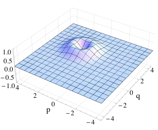
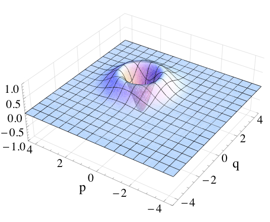
Figure 2: Wigner function ($\times\pi$, $\hbar=\omega=1$) of the beam splitter output 3, Eq. (20). It is a statistical mixture between a coherent state and a displaced Fock state. (a) 50:50 beam splitter ($t=1/\sqrt{2}$) with the coherent input state $\ket{\alpha=\sqrt{2}e^{i\pi/4}}$. (b) Highly reflective beam splitter ($t=1/10$) with the coherent input state $\ket{\alpha=10e^{i\pi/4}}$. Note, that $t\alpha$ is identical for both (a) and (b).

We have thus established an exact theory for the experiment of creating a displaced Fock state Lvovsky instead of the theory which the experiment was originally based on Banaszek ; Wallentowitz ; Mancini or the theory in Matteo .

II.3 Input: Coherent state and a general state

For future theoretical considerations and experimental demonstrations it might be useful to replace the ideal Fock state by a general state

$$\ket{\psi}_{0}=\sum_{m=0}^{\infty}c_{m}\ket{m}.$$ (24)

The input state then reads

$$\ket{\psi}_{0}\ket{\alpha}_{1}=\hat{D}_{1}(\alpha)\sum_{m=0}^{\infty}c_{m}\frac{1}{\sqrt{m!}}\left(\hat{a}_{0}^{\dagger}\right)^{m}\ket{0}_{0}\ket{0}_{1}\,\,\,.$$ (25)

It is straightforward to see that the output mode 3 of the BS is given by an equation analogous to Eq. (II.1), whereby the density matrix $\hat{\tilde{\rho}}_{23}$ becomes

$$\hat{\tilde{\rho}}_{23}=\sum_{m=0}^{\infty}\sum_{l=0}^{\infty}\frac{1}{\sqrt{m!l!}}c_{m}c_{l}^{*}(t^{\prime}\hat{a}_{2}^{\dagger}+r^{\prime}\hat{a}_{3}^{\dagger})^{m}\ket{0}_{2}\ket{0}_{3}\bra{0}_{3}\bra{0}_{2}(t^{\prime*}\hat{a}_{2}+r^{\prime*}\hat{a}_{3})^{l}.$$ (26)

Similar to above $\hat{\tilde{\rho}}_{23}$ is the non displaced density operator which would emerge at the output if the coherent state at the input would be replaced by vacuum. Thus the coherent input state displaces any state at the individual output port of a beam splitter compared to a vacuum input (see Eq. (II.1)). In the limit of a highly reflective beam splitter ($t\rightarrow 0$) Eq. (26) becomes $\hat{\tilde{\rho}}_{23}\rightarrow\ket{0}_{2}\ket{\psi}_{3}\bra{\psi}_{3}\bra{0}_{2}$. If we furthermore consider a strong coherent state ($t\alpha$ finite), we see from Eq. (II.1) that the effect on an arbitrary input state is approximately a mere displacement by $t\alpha$ of this state. A similar result has already been shown using a different approach in Matteo confirming our calculations.

III Interference at a Mach-Zehnder Interferometer

Now we consider a single-photon Fock state and a coherent state at the input of a Mach-Zehnder interferometer (MZI) as shown in Fig. 3. Again we want to calculate the quantum state at the output ports.

Figure 3: Mach-Zehnder Interferometer (MZI) with a phase shift in path 3. The input states at $BS_{1}$ are a single photon Fock state $\ket{1}_{0}$ and a coherent state $\ket{\alpha}_{1}$.

III.1 MZI scattering matrix

As suggested in Yurke , a MZI can be considered as a lossless and passive four port device. The annihilation operators of the field states transform similar to Eq. (9) and yield

$$\begin{pmatrix}\hat{a}_{4}\\ \hat{a}_{5}\end{pmatrix}=B_{MZI}\begin{pmatrix}\hat{a}_{0}\\ \hat{a}_{1}\end{pmatrix}.$$ (27)

The necessary and sufficient condition for the scattering matrix $B_{MZI}$ is that it has to be unitary. In fact, since we have already considered a general scattering matrix in the case of the beam splitter, Eq. (9), which essentially accounts for all passive and lossless four port devices, the calculations from the last section are generally valid. The scattering matrix of an arbitrary four port MZI, in particular, may be represented as a composition of several unitary scattering matrices.

The scattering matrix for the MZI, depicted on Fig.3 is composed of 3 unitary matrices, two matrices corresponding to the two beam splitters (see Eq. (9)) and one matrix associated with the phase shift, which in our case reads

$$U_{\theta}=\begin{pmatrix}1&0\\ 0&e^{i\theta}\end{pmatrix}.$$ (28)

Accordingly the annihilation operators of the field states transform as

$$\begin{pmatrix}\hat{a}_{4}\\ \hat{a}_{5}\end{pmatrix} =\begin{pmatrix}t_{2}&r_{2}^{\prime}\\ r_{2}&t_{2}^{\prime}\end{pmatrix}\begin{pmatrix}1&0\\ 0&e^{i\theta}\end{pmatrix}\begin{pmatrix}t_{1}^{\prime}&r_{1}\\ r_{1}^{\prime}&t_{1}\end{pmatrix}\begin{pmatrix}\hat{a}_{0}\\ \hat{a}_{1}\end{pmatrix}$$

$$=\begin{pmatrix}t^{\prime}_{M}&r_{M}\\ r^{\prime}_{M}&t_{M}\end{pmatrix}\begin{pmatrix}\hat{a}_{0}\\ \hat{a}_{1}\end{pmatrix}=B_{MZI}\begin{pmatrix}\hat{a}_{0}\\ \hat{a}_{1}\end{pmatrix},$$ (29)

where in the last line we defined the following variables:

$$r_{M}=r_{1}t_{2}+e^{i\theta}t_{1}r_{2}^{\prime},$$

$$t_{M}=r_{1}r_{2}+e^{i\theta}t_{1}t_{2}^{\prime},$$

$$r^{\prime}_{M}=t_{1}^{\prime}r_{2}+e^{i\theta}r_{1}^{\prime}t_{2}^{\prime},$$

$$t^{\prime}_{M}=t_{1}^{\prime}t_{2}+e^{i\theta}r_{1}^{\prime}r_{2}^{\prime}.$$ (30)

The variables defined in Eq. (III.1) obey the reciprocity relations Eq. (10), in particular $|t_{M}|=|t^{\prime}_{M}|$ and $|r_{M}|=|r^{\prime}_{M}|$.

Here we add a short comment with respect to Fig.3. The output ports $4$ and $5$ can serve as two paths of a second MZI including a second phase shift, subsequently followed by a third MZI of a similar type. Such a cascade of $3$ interferometers can operate as preparation, distribution and measuring module of a simple linear optical gate helpful in quantum computing systems. The resulting scattering matrix of such a device would be a matrix product of $3$ matrices similar to $B_{MZI}$ used in Eq. (III.1).

III.2 MZI Output states

The states at the output ports 4 and 5 of the MZI can now be calculated analogously to the output states of the single beam splitter in the previous section. Therefore according to Eq. (13) and by replacing the beam splitter scattering matrix $B$ with the MZI scattering matrix $B_{MZI}$ we get for the MZI output state

$$\ket{1}_{0}\ket{\alpha}_{1}\xrightarrow{MZI}\hat{D}_{4}(r_{M}\alpha)\hat{D}_{5}(t_{M}\alpha)(t^{\prime}_{M}\hat{a}_{4}^{\dagger}+r^{\prime}_{M}\hat{a}_{5}^{\dagger})\ket{0}_{4}\ket{0}_{5}.$$ (31)

Further we get for the reduced density matrix at output port 5 (compare with Eq. (17)),

$$\hat{\rho}_{5}=\left|t_{M}\right|^{2}\ket{t_{M}\alpha}_{5}\bra{t_{M}\alpha}_{5}+\left|r_{M}\right|^{2}\hat{D}_{5}(t_{M}\alpha)\ket{1}_{5}\bra{1}_{5}\hat{D}_{5}^{\dagger}(t_{M}\alpha)$$ (32)

and output port 4

$$\hat{\rho}_{4}=\left|r_{M}\right|^{2}\ket{r_{M}\alpha}_{4}\bra{r_{M}\alpha}_{4}+\left|t_{M}\right|^{2}\hat{D}_{4}(r_{M}\alpha)\ket{1}_{4}\bra{1}_{4}\hat{D}_{4}^{\dagger}(r_{M}\alpha).$$ (33)

The result is again, as in the case of the beam splitter, a mixed state between a coherent state (displaced vacuum) and a displaced Fock state, both displacements being identical. The Wigner function of this state can be calculated using the analogue of Eq. (20). The calculations where a coherent state and a general state are incident on a MZI are equivalent to the beam splitter case, so the output state is again merely displaced compared to a MZI with vacuum input instead of the coherent input state.

III.3 Photon numbers

Finally we calculate the average photon number at the output ports of the MZI. For port 5 it is defined as

$$\left<n\right>_{5}=\operatorname{Tr}_{5}(\hat{n}_{5}\hat{\rho}_{5})=\sum_{n=0}^{\infty}\left<n\vphantom{\hat{a}^{\dagger}_{5}\hat{a}_{5}\hat{\rho}_{5}n}\right|\hat{a}^{\dagger}_{5}\hat{a}_{5}\hat{\rho}_{5}\left|n\vphantom{n\hat{a}^{\dagger}_{5}\hat{a}_{5}\hat{\rho}_{5}}\right>_{5}.$$ (34)

For the coherent state we obtain, of course,

$$\sum_{n=0}^{\infty}\left<n\vphantom{\hat{a}^{\dagger}_{5}\hat{a}_{5}{t_{M}\alpha}}\right|\hat{a}^{\dagger}_{5}\hat{a}_{5}\left|{t_{M}\alpha}\vphantom{n\hat{a}^{\dagger}_{5}\hat{a}_{5}}\right>_{5}\Big{\langle}{t_{M}\alpha}\Big{|}n\Big{\rangle}_{5}=\left<{t_{M}\alpha}\vphantom{\hat{a}^{\dagger}_{5}\hat{a}_{5}{t_{M}\alpha}}\right|\hat{a}^{\dagger}_{5}\hat{a}_{5}\left|{t_{M}\alpha}\vphantom{{t_{M}\alpha}\hat{a}^{\dagger}_{5}\hat{a}_{5}}\right>_{5}=\left|{t_{M}\alpha}\right|^{2}.$$ (35)

For the displaced Fock state we obtain

$$\sum_{n=0}^{\infty}\left<n\vphantom{\hat{a}^{\dagger}_{5}\hat{a}_{5}D_{5}({t_{M}\alpha})1}\right|\hat{a}^{\dagger}_{5}\hat{a}_{5}D_{5}({t_{M}\alpha})\left|1\vphantom{n\hat{a}^{\dagger}_{5}\hat{a}_{5}D_{5}({t_{M}\alpha})}\right>_{5}\left<1\vphantom{\hat{D}_{5}^{\dagger}({t_{M}\alpha})n}\right|\hat{D}_{5}^{\dagger}({t_{M}\alpha})\left|n\vphantom{1\hat{D}_{5}^{\dagger}({t_{M}\alpha})}\right>_{5}$$

$$=\left<1\vphantom{\hat{D}_{5}^{\dagger}(t_{M}\alpha)\hat{a}^{\dagger}_{5}\hat{a}_{5}\hat{D}_{5}(t_{M}\alpha)1}\right|\hat{D}_{5}^{\dagger}(t_{M}\alpha)\hat{a}^{\dagger}_{5}\hat{a}_{5}\hat{D}_{5}(t_{M}\alpha)\left|1\vphantom{1\hat{D}_{5}^{\dagger}(t_{M}\alpha)\hat{a}^{\dagger}_{5}\hat{a}_{5}\hat{D}_{5}(t_{M}\alpha)}\right>_{5}=1+\left|{t_{M}\alpha}\right|^{2},$$ (36)

where in the last step the commutation relation M&W $\hat{a}\hat{D}({t_{M}\alpha})=$ $\hat{D}({t_{M}\alpha})(\hat{a}+{t_{M}\alpha})$ has been used. With the last two equations and using that $\left|t_{M}\right|^{2}+\left|r_{M}\right|^{2}=1$ we can now calculate the average photon number, Eq. (34), and get

$$\left<n\right>_{5}=\left|t_{M}\right|^{2}\left|{t_{M}\alpha}\right|^{2}+\left|r_{M}\right|^{2}\left(1+\left|{t_{M}\alpha}\right|^{2}\right)=\left|r_{M}\right|^{2}+\left|{t_{M}\alpha}\right|^{2}.$$ (37)

For port 4 we get analogously

$$\left<n\right>_{4}=\left|t_{M}\right|^{2}+\left|{r_{M}\alpha}\right|^{2}.$$ (38)

Using this formalism the mean square deviation $\langle(\Delta{}n)^{2}\rangle=\langle{}n^{2}\rangle-\langle{}n\rangle^{2}$ of photons can be calculated leading to

$$\langle(\Delta{}n)^{2}\rangle_{5}=|t_{M}\alpha|^{2}(1+2|r_{M}|^{2})+|r_{M}|^{2}|t_{M}|^{2}\,\,\,,$$

$$\langle(\Delta{}n)^{2}\rangle_{4}=|r_{M}\alpha|^{2}(1+2|t_{M}|^{2})+|r_{M}|^{2}|t_{M}|^{2}\,\,\,$$ (39)

for the two output ports.

III.4 Discussion of a MZI with balanced BSs

As a particular example, that can be realized easily in an experiment, we calculate the average photon numbers for the case of two 50:50 dielectric layer beam splitters with a phase factor of $e^{i\pi/2}=i$ for the reflected beams ($t_{1}=t^{\prime}_{1}=t_{2}=t^{\prime}_{2}=1/\sqrt{2},\,r_{1}=r^{\prime}_{1}=r_{2}=r_{2}^{\prime}=i/\sqrt{2}$) BSHamilton . In this case the transmittivity and the reflectivity are $|t_{M}|^{2}=\sin^{2}(\theta/2)$ and $|r_{M}|^{2}=\cos^{2}(\theta/2)$. Both are completely determined by $\theta$. The average photon numbers are then

$$\left<n\right>_{4}=\sin^{2}(\theta/2)+\left|\alpha\right|^{2}\cos^{2}(\theta/2),$$ (40)

$$\left<n\right>_{5}=\cos^{2}(\theta/2)+\left|\alpha\right|^{2}\sin^{2}(\theta/2)$$ (41)

and the mean square deviations are given by

$$\langle(\Delta{}n)^{2}\rangle_{4}=\frac{1}{4}\sin^{2}(\theta)+|\alpha|^{2}[\cos^{2}(\frac{\theta}{2})+\frac{1}{2}\sin^{2}(\theta)]\,\,\,,\,\,\,\langle(\Delta{}n)^{2}\rangle_{4}-\langle(\Delta{}n)^{2}\rangle_{5}=|\alpha|^{2}\cos(\theta)\,.\,\,\,\,\,\,\,\,\,\,\,\,$$ (42)

Figure 4 shows the average photon numbers as a function of the phase shift $\theta$ for different coherent input states $\ket{\alpha}$. The maxima and minima in the graph indicate the cases where the quantum states at the separate output ports are either a pure coherent state or a pure Fock state.

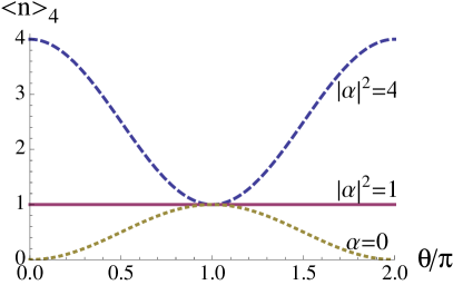
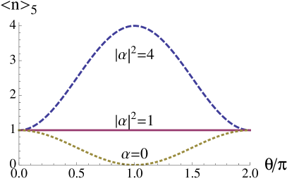
Figure 4: Average photon number at output 4 (a) and output 5 (b) of the Mach Zehnder Interferometer with the coherent input states $\ket{\left|\alpha\right|=0}$, $\ket{\left|\alpha\right|=1}$ and $\ket{\left|\alpha\right|=2}$. Note that for $|\alpha|^{2}=1$ the mean photon numbers are independent of $\theta$ and equal to 1.

The technical advantage of the MZI (with two 50:50 BSs) over a single beam splitter is, that ${t_{M}}$ and ${r_{M}}$ can simply be adjusted by changing the phase $\theta$ in path 3. All desired states could be generated in experiments without changing the setup by selecting another beam splitter with the appropriate transmittivity $\left|t\right|^{2}$ and reflectivity $\left|r\right|^{2}$.

Let us compare the result for $|\alpha|^{2}=1$ with the case when two separate single-photon Fock states are impinging on the input ports of an MZI. The first balanced $BS_{1}$ of the latter is reminiscent to the Hong-Ou-Mandel (HOM) effect HongOuMandel . After the $BS_{1}$ the state is $\,i(|2\rangle_{2}|0\rangle_{3}+|0\rangle_{2}|2\rangle_{3})/\sqrt{2}\,$ which means that no coincidences appear behind $BS_{1}$ Knight . Introducing a phase shift $\theta$ in path 3 and a second $BS_{2}$ (see fig. 3) the wave function behind the MZI reads

$$|\psi\rangle=\frac{1}{2\sqrt{2}}\{(1-e^{2i\theta})[\,|0\rangle_{4}|2\rangle_{5}-|2\rangle_{4}|0\rangle_{5}]+\sqrt{2}(1+e^{2i\theta})|1\rangle_{4}|1\rangle_{5}\}\,\,.$$ (43)

The probability for coincidences is $W_{45}=\cos^{2}(\theta)$ while the probabilities of measuring 2 photons at the output ports 4 and 5 are $W_{4}=W_{5}=\frac{1}{2}\sin^{2}(\theta)$. However, the mean photon numbers $\langle{}n\rangle_{4}^{|\psi\rangle}$ and $\langle{}n\rangle_{5}^{|\psi\rangle}$ are equal to 1 and therefore independent of $\theta$. This can be compared with the results of the present paper (see Eqs. (40) and (41)) in which the mean photon numbers in output 4 and 5 also do not depend on $\theta$. Anyway, one has to keep in mind that these two examples have completely different initial conditions although the input mean photon numbers are the same in case of $|\alpha|^{2}=1$. In fact, one has to compare the entangled quantum states of the HOM-effect Eq. (43) on the one hand with the MZI-state Eq. (31) on the other hand and realize that these are completely different. By executing the trace operation for the separate output ports, however, entanglement is eliminated in both cases yielding the identical outcomes for the mean photon numbers.

IV Summary and outlook

To sum up, we have derived simple analytical solutions for a quantum state and its Wigner function at the output ports of a general passive and lossless optical four port like a beam splitter, when a coherent state and a single-photon Fock state are incident on the input ports. These calculations could be of interest in the fields of quantum cryptography based on continuous variables and optical quantum computing. We have obtained a statistical mixture between of a coherent state and a displaced Fock state and have derived the corresponding Wigner functions. Furthermore, we have shown that a coherent input state displaces the quantum state at the output port of a beam splitter in phase space as compared with vacuum at the input port, when in both cases a general state is incident on the second input port. Additionally, we have analyzed the quantum states behind a Mach-Zehnder interferometer and have evaluated mean photon numbers at the output ports. It turns out that for an input state $|1\rangle_{0}||\alpha|=1\rangle_{1}$ the mean photon numbers behind the MZI do not depend on the phase shift $\theta$ inserted in the interferometer.

In addition to the $3$-interferometer-cascade mentioned in section III/A a further possible application of the presented formalism can be proposed. Instead of the reflector $R$ in path $2$ of Fig. 3 a beam splitter can be inserted in such a way that beam $2$ is both reflected and transmitted. The beam splitter provides also an additional input. A second MZI then can be added below the first one. In particular these two interferometers have one beam path in common generating a so-called two-loop interferometer which consists of $4$ beam splitters and $2$ reflectors providing $3$ input and $3$ output ports. Such a device enables the superposition of three wave functions and will be theoretically investigated in a next step.

The results of this paper can serve as a basis for further phase-space investigations of higher Fock states in combination with coherent, squeezed or thermal states as input states used in current optical setups. Those setups (BS, MZI, Phase gate, CNOT gate) are building blocks for linear optical quantum computers.

References

• (1) M. Dǔsek, N. Lütkenhaus, and M. Hendrych, “Quantum Cryptography,” Progress in Optics 49 (2006) 381, quant-ph/0601207.
• (2) J. Lodewyck, M. Bloch, and R. G.-P. et al., “Quantum key distribution over 25 km with an all-fiber continuous-variable system,” Phys. Rev. A 76 (2007) 042305, arXiv:0706.4255 [quant-ph].
• (3) M. A. Nielsen and I. L. Chuang, Quantum Computation and Quantum Information. Cambridge University Press, Cambridge, 2000.
• (4) N. Gisin, G. Ribordy, W. Tittel, and H. Zbinden, “Quantum Cryptography,” Rev. Mod. Phys 74 (2002) 145, quant-ph/0101098.
• (5) J. L. O’Brien, “Optical Quantum Computing,” Science 318 (2007) 1567, arXiv:0803.1554 [quant-ph].
• (6) A. Politi, M. J. Cryan, J. G. Rarity, S. Yu, and J. L. O’Brien, “Silica-on-Silicon Waveguide Quantum Circuits,” Science 320 (2008) 646, arXiv:0802.0136 [quant-ph].
• (7) L. Mandel and E. Wolf, Optical Coherence and Quantum Optics. Cambridge Univ. Press, Cambridge, 1995.
• (8) U. Leonhardt, “Quantum Physics of Simple Optical Instruments,” Rept.Prog.Phys. 66 (2003) 1207, quant-ph/0305007.
• (9) B. Yurke, S. L. McCall, and J. R. Klauder, “SU(2) and SU(1) interferometers,” Phys. Rev. A 33 (1986) 4033.
• (10) C. C. Gerry and P. L. Knight, Introductory Quantum Optics. Cambridge Univ. Press, Cambridge, 2005.
• (11) C. K. Hong, Z. Y. Ou, and L. Mandel, “Measurement of Subpicosecond Time Intervals between Two Photons by Interference,” Phys. Rev. Lett. 59 (1987) 2044.
• (12) C. K. Hong, Z. Y. Ou, and L. Mandel, “Interference between a fluorescent photon and a classical field: An example of nonclassical interference,” Phys. Rev. A 37 (1988) 3006.
• (13) S. Bali, F. A. Narducci, and L. Mandel, “Coherence and elastic scattering in resonance fluorescence,” Phys. Rev. A 47 (1993) 5056.
• (14) A. I. Lvovsky and S. Babichev, “Synthesis and Tomographic Characterization of the displaced Fock state of light,” Phys. Rev. A 66 (2002) 011801, quant-ph/0202163.
• (15) M. W. Hamilton, “Phase shifts in multilayer dielectric beam splitters,” Am. J. Phys. 68 (2000) 186.
• (16) G. G. Stokes Cambridge & Dublin Math. J. 4 (1849) 1.
• (17) F. A. M. de Oliveira, M. S. Kim, P. L. Knight, and V. Bušek, “Properties of displaced number states,” Phys. Rev. A 41 (1990) 2645.
• (18) E. Wigner, “On the Quantum Correction For Thermodynamic Equilibrium,” Phys. Rev. 40 (1932) 749.
• (19) M. Hillary, R. F. O’Connell, M. O. Scully, and E. P. Wigner, “Distribution Function in Physics: Fundamentals,” Phys. Rep 106 (1984) 121–167.
• (20) W. P. Schleich, Quantum Optics in Phase Space. Wiley-Vch, Berlin, 2001.
• (21) M. Suda, Quantum Interferometry in Phase Space. Springer, Berlin, 2006.
• (22) U. Leonhardt, Measuring the Quantum State of Light. Cambridge Univ. Press, Cambridge, 1997.
• (23) K. Banaszek and K. Wodkiewicz, “Direct Probing of Quantum Phase Space by Photon Counting,” Phys. Rev. Lett. 76 (1996) 4344, atom-ph/9603003.
• (24) S. Wallentowitz and W.Vogel, “Unbalanced Homodyning for Quantum State Measurements,” Phys. Rev. A 53 (1996) 4528.
• (25) S. Mancini, P. Tombesi, and V. Manko, “Density Matrix from Photon Number Tomography,” Europhys. Lett. 37 (1997) 79, quant-ph/9612004.
• (26) M. G. A. Paris, “Displacement operator by beam splitter,” Phys. Lett. A 217 (1996) 78–80.