A small probabilistic universal set of starting points for finding roots of complex polynomials by Newton’s method

Abstract.

We specify a small set, consisting of $O(d(\log\log d)^{2})$ points, that intersects the basins under Newton’s method of all roots of all (suitably normalized) complex polynomials of fixed degrees $d$, with arbitrarily high probability. This set is an efficient and universal probabilistic set of starting points to find all roots of polynomials of degree $d$ using Newton’s method; the best known deterministic set of starting points consists of $\lceil 1.1d(\log d)^{2}\rceil$ points.

1. Introduction

Newton’s root-finding method is as old as analysis, but still not well understood, even in the fundamental case of finding all roots of a polynomial in a single variable. Its local convergence properties are well known; near simple roots convergence is quadratic and thus extremely rapid. However, the global dynamical properties are insufficiently understood so that numerical analysis algorithms often use different global methods, and resort to Newton’s method for a final local “polishing” of the roots.

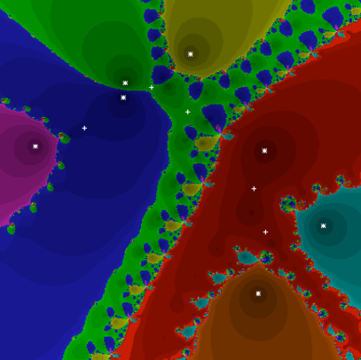
This article is a contribution towards a better understanding of the global properties of Newton’s method, applied to polynomials in a single complex variable. Even for polynomials over the reals, and even if all the roots are real, it is often preferable to use complex methods; see Figure 1.

Figure 1. Dynamical planes of Newton maps of two complex polynomials. Different colors illustrate basins of attraction of different roots; shades of color illustrate different speeds of convergence. It is clearly visible that all immediate basins are unbounded and have one or several channels to $\infty$ of different widths. Left: a polynomial of degree $7$. Right: a polynomial of degree $11$ with all roots real. Some of the roots are very close to each other; however, away from the disk containing all the roots, the basins and their channels all have almost uniform width, so that finding the real roots using complex methods is much easier.

Figure 2. The dynamical plane of the polynomial $p(z)=z(z^{10}-1)$: the ten roots of unity each have one “thick” channel, while the root $z=0$ has 10 channels (red) which are all rather “thin”. The deterministic method from [HSS] would search for the individual thin channels and thus requires more points, while our method searches for the union of all thin channels, which together are much bigger.

Among the difficulties with Newton’s method are the following:

• if an orbit under iteration comes close to a critical point of the polynomial, the Newton map sends the orbit far away near $\infty$, so that control of the dynamics is lost, and in any case a large number of iterations are required until the orbit comes back to where the roots are;

• there are polynomials with open sets of starting points that do not converge to any root (Smale [S1] asked, in 1984, for a classification of such polynomials; an answer has recently been given by Mikulich in current work [Mi]);

• the boundary of the basins of convergence for the roots may have positive planar Lebesgue measure (this follows from recent work by Buff and Chéritat on the existence of Julia sets with positive measure [BC], combined with Douady and Hubbard’s renormalization theory [DH]);

• even if almost every point in $\mathbb{C}$ converges to some root under the Newton iteration, our goal is to find all roots of the polynomial, and with bounded complexity. Finding some roots and deflating is usually not an option, because deflation is in general numerically unstable (unless the roots are found in a specific order), and because deflation might not be compatible with the way the polynomial may be specified, or evaluated efficiently (for instance, if the polynomial itself is given by an efficient iteration procedure).

See [Rü] for a recent survey of known results on Newton’s method.

This article is a contribution towards the goal of turning Newton’s method into an efficient algorithm. To achieve this goal, one should:

• select a finite set $\mathcal{S}_{d}$ of good starting points that are guaranteed to intersect the basins of all roots;

• specify a condition when to stop iterating any of these starting points, because the orbit is either sufficiently close to a root, or the orbit is discarded in favor of some other starting points;

• give a good bound on the complexity of Newton’s method to find all roots of the polynomial with prescribed precision.

This article is concerned with the first of these questions; we will not discuss the other two issues in detail (see for instance [S2, Rü]). Concerning efficiency of the Newton method, we mention the following recent result from [Sch1, Sch2, ABS]: roughly speaking, for “most” polynomials $p$ of degree $d$, properly normalized, our universal set $\mathcal{S}_{d}$ contains $d$ points that converge to the $d$ different roots of $p$ so that the total number of Newton iterations, for all $d$ roots combined, to achieve an accuracy of $\varepsilon$ is at most $O(d^{2}\log^{4}d)+d\log|\log\varepsilon|$. This makes it possible to turn Newton’s method into an efficient algorithm for the problem of finding all roots of a given polynomial.

To state our main result, let $\mathcal{P}_{d}$ be the space of polynomials of degree $d$, normalized so that all roots are contained in the complex unit disk $\mathbb{D}$.

Theorem 1 (Small Probabilistic Universal Set of Starting Points).

For every degree $d\geq 3$, there is an explicit universal probabilistic set $\mathcal{S}_{d}$ consisting of $O(d(\log\log d)^{2})$ starting points so that for every polynomial $p\in\mathcal{P}_{d}$, the probability is greater than $1/2$ that the immediate basin of each root of $p$ contains at least one point in $\mathcal{S}_{d}$ (in fact, this probability is greater than $1-1/d\geq 2/3$).

Remark 1.

The meaning of an “explicit and universal” probabilistic set is as follows: we give an explicit probability distribution of starting points that depends only on $d$ so that for any $p\in\mathcal{P}_{d}$, with probability at least $1-1/d$ all immediate basins contain at least one point in this set. (The probability $1-1/d$ may seem somewhat artificial; it is what we get naturally from of our estimates, and it is better than the uniform $2/3$.) Of course, enlarging this set of points appropriately, the probability of success can be increased (see Remark 7): For every probability $\rho\in(0,1)$, there is an explicit and universal set $\mathcal{S}_{d,\rho}$ of starting points with cardinality $O\big{(}d(\log\log d)^{2}+d|\log(1-\rho)|\big{)}$ such that the statement of Theorem 1 is true with probability $\rho$ instead of $1-1/d$.

This result is in a similar spirit as [HSS], where a similar explicit universal set of starting points is constructed. It consists of $\lceil 1.1d(\log d)^{2}\rceil$ points and is deterministic. Our new set is significantly smaller than the deterministic set, much closer to the “ideal lower bound” of $d$ points, but we can do so only using a probabilistic set. We believe that there is no deterministic explicit and universal set of starting points with $o(d\log d)$ points.

Construction of the set $\mathcal{S}_{d}$. Our set $\mathcal{S}_{d}$ is constructed as follows: firstly, we define a “fundamental annulus” $V:=\left\{z\in\mathbb{C}\colon R\sqrt{1-1/d}<z<R\right\}$ for some $R>1+\sqrt{2}$, and choose a “deterministic set” of approximately $(16/\pi)d(\log\log d)^{2}$ points that are distributed on $m=\lceil(2/\pi)\log\log d\rceil$ circles. These circles have radii $R_{k}=R(1-1/d)^{(k-1/2)/2m}$ for $k=0,1,,\dots,m-1$, and each circle contains $\lceil 4\pi d\lceil(2/\pi)\log\log d\rceil\rceil$ points at equal distances. This construction is in principle the same as in [HSS]. Secondly, we choose a “probabilistic set” of $\lceil(300/\pi)d\log\log d\rceil$ points randomly inside the annulus $A_{R}=\{z\in\mathbb{C}\colon R(d-1)/d-1/d<|z|<R\}$ for some $R\geq 11$. These deterministic and probabilistic sets of points will respectively find “thick” and “thin” roots, as defined below. Iterating Newton’s method starting at these points (in parallel or in any order), we will find all roots of $p$ with probability at least $1-1/d$ (or with any probability $\rho\in(0,1)$ when taking appropriately more points in the probabilistic set).

Historical Remark. This research has its origins at the 50th anniversary celebration of the International Mathematical Olympiad (IMO) held in 2009 in Bremen, Germany. One chief goal of this celebration was to bring together olympiad mathematics and research mathematics, and people involved in both. This paper was authored by a research mathematician who in his youth was one of the first contestants ever at IMOs and in 2009 was a guest of honor at the 50th IMO, together with one of the contestants there, and a research mathematician who was among the senior organizers of that IMO and its anniversary. This work is thus very much in the spirit of the IMO anniversary, and we are grateful to this anniversary celebration that has brought us together.

We gratefully acknowledge partial support through NSF grants DMS-0906634, CNS-0721983 and CCF-0728928, ARO grant W911NF-06-1-0076, and the TAMOP-4.2.2/08/1/2008-0008 program of the Hungarian National Development Agency (BB), as well as the European Research and Training network CODY, the ESF programme HCAA, and the German Research Council DFG (DS). We also gladly acknowledge useful feedback from an anonymous referee.

2. Channels and Their Moduli

Consider a complex polynomial $p(z)=c\prod_{j=1}^{d}(z-\alpha_{j})$ and let $N_{p}(z)=z-p(z)/p^{\prime}(z)$ be the associated Newton map. This is a rational map of degree $d$ if all roots of $p$ are distinct, and of lower degree otherwise. Without changing the Newton map, we may suppose that $c=1$, and after rescaling, we may suppose that all $\alpha_{j}\in\mathbb{D}$.

For any root $\alpha$ of $p$, let $U_{\alpha}$ be the immediate basin of $\alpha$: the basin is the set of all $z\in\mathbb{C}$ that converge to $\alpha$ under iteration of $N_{p}$, and the immediate basin is the connected component containing $\alpha$. It is known that each $U_{\alpha}$ is simply connected [Pr] and that the restriction of $N_{p}$ to $U_{\alpha}$ sends $U_{\alpha}$ to itself as a proper map of some degree $k+1\in\{2,3,\dots,d\}$. We will use the construction and some results from [HSS]. If $\varphi\colon U_{\alpha}\to\mathbb{D}$ is a Riemann map with $\varphi(\alpha)=0$, then $f:=\varphi\circ N_{p}\circ\varphi^{-1}$ is a proper holomorphic self-map of $\mathbb{D}$ of degree $k+1$ and thus extends, by Schwarz reflection, to a rational map of degree $k+1$, and the restriction of $f$ to $\partial\mathbb{D}$ is a covering of $\partial\mathbb{D}$, also of degree $k+1$. In particular, the restriction of $f$ to $\partial\mathbb{D}$ has $k\geq 1$ fixed points $q_{1},\dots,q_{k}$. Set $\lambda_{i}:=f^{\prime}(q_{i})$, for $i=1,2,\dots,k$.

The holomorphic fixed point formula (which essentially is the residue theorem for $1/(z-f(z))$; see [M]) implies that

(1) $$\sum_{i=1}^{k}\frac{1}{\lambda_{i}-1}\geq 1$$

(with equality if the root $\alpha$ is simple). Each of these $k$ fixed points gives rise to a channel to $\infty$ in the immediate basin $U_{\alpha}$: for our purposes, a channel is an unbounded component $B_{i}$ of $U_{\alpha}\setminus\overline{\mathbb{D}}$. Near $\infty$, each channel is mapped by $N_{p}$ conformally to itself, and it defines an access to $\infty$ within $U_{\alpha}$ that is fixed by $N_{p}$. The quotient of $B_{i}$ by the dynamics of $N_{p}$ is a conformal annulus with modulus $\mu_{i}=\pi/\log\lambda_{i}$.

Choose some positive real number $M<\pi/\log 4\approx 2.266$ that will be specified later (we will eventually use $M=\pi/\log\log d$ for large $d$).

We call a root $\alpha$ thick if it has a channel with modulus $\mu_{i}\geq M$, and thin if there is no such channel. We will treat these two cases separately.

• We will explicitly and deterministically construct a set of $\lceil 4\pi d\lceil 2/M\rceil^{2}\rceil$ points that is guaranteed to intersect each channel of a root with modulus greater than $M$. This set will thus suffice to “find” all thick roots.

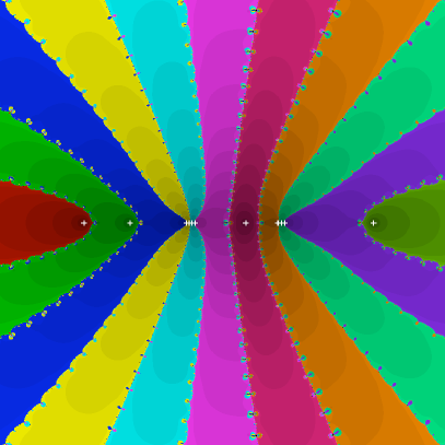
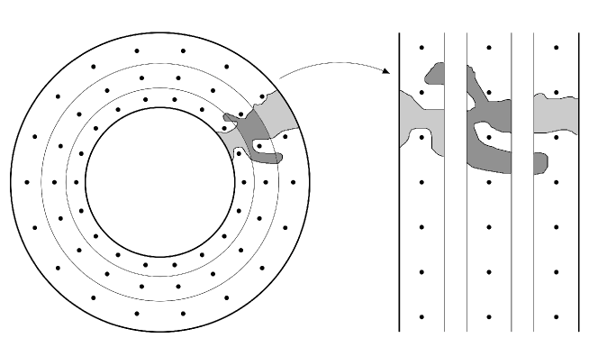
• The advantage of thin roots is that even though the individual channels have small moduli, the total area of these channels within any fundamental domain of the Newton dynamics is greater than in the thick case: each channel may have little area, but there are more channels in this case (see Figure 2). We show that if $\lceil 300\,d\log d/Me^{\pi/M}\rceil$ points are distributed randomly in a certain fundamental annulus of the Newton dynamics, then the probability that the immediate basins of all thin roots contain such a point is at least $1-1/d$.

Remark 2.

If $\alpha$ is a thin root, then all $\mu_{i}<M$, hence all $\lambda_{i}-1=e^{\pi/\mu_{i}}-1>e^{\pi/M}-1$, so by (1), the number $k$ of channels of a thin root is strictly greater than $e^{\pi/M}-1$. But the mapping degree of $U_{\alpha}$ equals $k+1$, so $U_{\alpha}$ must contain $k>e^{\pi/M}-1$ of the at most $2d-2$ critical points of $N_{p}$, and thus the number of thin roots is at most $(2d-2)/(e^{\pi/M}-1)$. In the end, we will use $M=\pi/\log\log d$, so the number of thin roots will be at most $(2d-2)/(\log d-1)$: most roots will be thick. It seems to be an interesting question (outside the scope of this paper) to estimate how likely it is for a given polynomial of degree $d$ to have all its roots thick.

If there are thin roots, then we can estimate

(2) $$e^{\pi/M}<k+1\leq d\;;$$

in particular, there are no thin roots at all if $M\leq\pi/\log d$.

A conformal quadrilateral is a Riemann domain $Q\subset\mathbb{C}$ with two distinguished connected and disjoint subsets of the boundary. In our setting, the boundary of $Q$ may not be a topological curve, but the two distinguished boundary subsets will be; we will call them distinguished boundary arcs. Then there is a unique $h>0$ so that the domain $Q_{h}:=\{z\in\mathbb{C}\colon 0<\text{\rm Im}\,z<1,0<\text{\rm Re}\,z<h\}$ has a Riemann map $\varphi\colon Q\to Q_{h}$ that maps the two distinguished boundary arcs onto the two horizontal sides of $Q_{h}$ (the Riemann map may not extend continuously to the boundary of $Q$, but it does so near the two distinguished boundary arcs; the general framework of extremal length using curve families works even if the boundaries are not curves). The value $h$ is defined as the conformal modulus of the quadrilateral $Q$ with respect to the two boundary subsets, and denoted $\operatorname*{mod}(Q)$; it is invariant for conformal homeomorphisms that respect the distinguished boundary subsets, in particular for Riemann maps with this property [A].

Identifying the two distinguished boundary arcs, we obtain a complex annulus (a doubly connected Riemann surface) with modulus $\operatorname*{mod}(Q)$ or less (the exact modulus depends on how the boundaries are identified).

3. Hitting thick roots

In this section, we will construct an explicit and deterministic set of starting points that is guaranteed to intersect the basins of all thick roots. Our arguments are essentially the same as in [HSS, Section 5], except that we no longer need to find all roots, but only the thick ones.

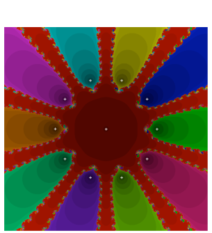
If $R>(d+1)/(d-1)$ and $C_{R}$ is the circle of radius $R$ centered at the origin, then $N_{p}$ maps $C_{R}$ homeomorphically onto some topological circle around $\mathbb{D}$, and there is some $\kappa>0$ so that the round annulus

$$V_{R,\kappa,d}=\left\{z\in\mathbb{C}\colon R\left(\frac{d-1}{d}\right)^{\kappa}<|z|<R\right\}$$

is contained in the topological annulus between $C_{R}$ and $N_{p}(C_{R})$; specifically, if $R\geq 1+\sqrt{2}$, then $\kappa\geq 1/2$ for all $d$. If $R$ tends to $\infty$, then $\kappa$ tends to $1$. All this is [HSS, Lemmas 4 and 12]; see also Figure 3.

Figure 3. Left: the dynamics of Newton’s method for some complex polynomial. Highlighted is the immediate basin of attraction of one root, with fundamental domains within the channels shaded. Also shown is the circle at radius $R$ and its image, which is a topological (but not geometric) circle. Right: the complex unit disk $\mathbb{D}$ provides a conformal model for the Newton dynamics of the immediate basin. (Picture taken from [HSS].)

We will use the round annulus $V=V_{R,\kappa,d}$ with $R\geq 1+\sqrt{2}$ and $\kappa=1/2$ (if we use larger values of $R$, then we can take larger values of $\kappa$, and our bounds will eventually be slightly better; however, in practice these starting points would be further away from the roots, and the iteration would take longer).

Remark 3.

The modulus of $V$ is $|\log((d-1)/d)|/4\pi>1/4\pi d$.

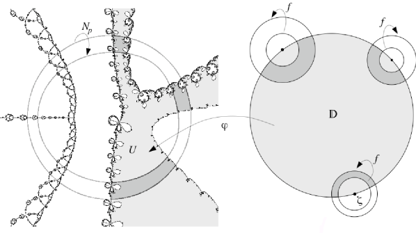
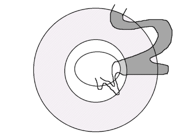
Consider some channel $B_{i}$. We want to define $Q_{i}$ as “the part of the channel $B_{i}$ within $V$”. If each of the two boundary circles of $V$ intersects $B_{i}$ in a single connected arc, we set $Q_{i}:=B_{i}\cap V$. However, if $B_{i}\setminus V$ has more than two connected components (see Figure 4), we need to be more careful. Consider the intersection of $B_{i}$ with $C_{R}$, the outer boundary of $V$. Let $\gamma$ be any connected component in this intersection. It separates $U_{\alpha}$ into two components, one of which contains the root $\alpha$; then $\gamma$ will be called an essential boundary arc of $B_{i}\cap C_{R}$ if the component of $U_{\alpha}\setminus\gamma$ not containing $\alpha$ is unbounded: this means that $\gamma$ separates the unbounded part of the channel $B_{i}$ from the root. At least one component of $B_{i}\cap C_{R}$ is essential; choose one such essential component $\gamma$, let $\gamma^{\prime}:=N_{p}(\gamma)$, and let $Q^{\prime}_{i}$ be the subset of $U_{\alpha}$ that is bounded by $\gamma$ and $\gamma^{\prime}$ (if $B_{i}$ intersects $C_{R}$ and equivalently $N_{p}(C_{R})$ in only one component, then $Q^{\prime}_{i}$ is the part of $B_{i}$ between $C_{R}$ and $N_{p}(C_{R})$; in general, the difference may consist of some number of bounded components). Then $Q^{\prime}_{i}$ is a fundamental domain of $B_{i}$ by the dynamics; when viewed as a quadrilateral with distinguished boundary arcs $\gamma$ and $\gamma^{\prime}$, then $\operatorname*{mod}(Q^{\prime}_{i})\geq\operatorname*{mod}(B_{i})=\mu_{i}$ ($Q^{\prime}_{i}$ is a quadrilateral, the modulus of $B_{i}$ is defined using the quotient annulus of $B_{i}$ by the dynamics).

Now let $C_{R^{\prime}}$ be the inner boundary circle of $V$ and consider all essential arcs of intersection of $B_{i}\cap C_{R^{\prime}}$. If there is only one, then let $\gamma^{\prime\prime}$ be this essential arc. If there are several, then they are totally ordered (because they all separate $\alpha$ in $U_{\alpha}$ from the unbounded component of $B_{i}\setminus V$). Let $\gamma^{\prime\prime}$ be the outermost component that separates $\alpha$ from $\gamma$ (i.e., the one closest to $\gamma$), and let $Q_{i}$ be the component of $B_{i}\setminus(\gamma\cup\gamma^{\prime\prime})$ that is bounded by $\gamma$ and $\gamma^{\prime\prime}$. This is a conformal quadrilateral with $Q_{i}\subset Q^{\prime}_{i}$, and with $\gamma$ and $\gamma^{\prime\prime}$ as distinguished boundary arcs, and we have $\operatorname*{mod}(Q_{i})\geq\operatorname*{mod}(Q^{\prime}_{i})\geq\mu_{i}$.

Figure 4. The annulus $V$ (hatched). Its outer boundary circle is $C_{R}$; the image $N_{p}(C_{r})$ is a topological circle within the bounded complementary component of $V$. Also shown is a channel $B_{i}$; it intersects $C_{R}$ in four arcs, three of which are essential. Shaded is the quadrilateral $Q^{\prime}_{i}$ which is bounded by two essential arcs, one on $C_{R}$ and one on $N_{p}(C_{R})$; it is a fundamental domain of $B_{i}$ modulo $N_{p}$. The quadrilateral $Q_{i}\subset Q^{\prime}_{i}$ is shaded darker: it is bounded by two essential arcs on $\partial V$, but may not be contained in $V$.

Our task will be to distribute sufficiently many points into $V$ so that we hit quadrilaterals $Q_{i}\subset V$ with moduli bounded below.

Lemma 2.

Let $S=\{z\in\mathbb{C}\colon-1/2<\text{\rm Re}\,z<1/2\}$ and let $Q\subset\mathbb{C}$ be a quadrilateral whose two distinguished boundary arcs are on the two vertical sides of $S$, one on each. Suppose that $Q$ is disjoint from the set $i\mathbb{Z}$. Then the modulus of $Q$ is at most $2$.

Proof.

This is an easy extremal length exercise [A]. There is an integer $n\in\mathbb{Z}$ so that any curve in $Q$ connecting the two distinguished boundary arcs must intersect the segment $[ni,(n+1)i]$. Without loss of generality, suppose that $n=0$.

Let $B:=\{z\in S\colon-1/2<\text{\rm Im}\,z<3/2\}$ and let $\rho$ be the characteristic function of $B$. Then for any curve $\gamma\subset Q$ connecting the two distinguished boundary arcs, its intersection with $B$ has length at least $1$. Since $\int_{\mathbb{C}}\rho^{2}\,dx\,dy=2$, it follows that $\operatorname*{mod}(Q)\leq 2$. ∎

Remark 4.

The bound of $2$ is not sharp. It is not hard to calculate the exact bound [A], but we are not optimizing constant factors here.

Lemma 3.

If $V$ is subdivided into at least $2/M$ concentric and conformally equivalent subannuli, and at least $4\pi d\lceil 2/M\rceil$ points are distributed onto the core circles of all subannuli, so that the points on all circles are equidistributed, then each quadrilateral $Q_{i}$ with modulus at least $M$ contains at least one of these points.

Proof.

Let $m:=\lceil 2/M\rceil$ and subdivide $V$ into $m$ concentric and conformally equivalent subannuli $V_{1},\dots,V_{m}$, ordered by decreasing radii (so that $V_{k}=\{z\in V\colon R\beta^{k}<|z|<R\beta^{k-1}\}$ for $\beta=(1-1/d)^{1/2m}$) . Write $Q$ for $Q_{i}$; this is a quadrilateral for which the two distinguished boundary arcs are on $\partial V$, one on each boundary component of $V$.

Subdivide $Q$ into quadrilaterals $Q^{\prime}_{1},\dots,Q^{\prime}_{m}$ as follows, similarly as above. The common boundary circle of $V_{j}$ and $V_{j+1}$ may intersect $Q$ in several arcs; such an arc is essential if it separates the root $\alpha$ from the unbounded component of $B_{i}\setminus V$. Use an essential arc to separate $Q^{\prime}_{j}$ from $Q^{\prime}_{j+1}$, for $j=1,2,\dots,m-1$. (In the special case that $B_{i}\cap\partial V_{j}$ only has two connected components, then simply $Q^{\prime}_{j}=B_{i}\cap V_{j}$.)

By the Grötzsch inequality, one of the quadrilaterals $Q^{\prime}_{j}$ has modulus $\operatorname*{mod}(Q^{\prime}_{j})\geq m\cdot\operatorname*{mod}(Q)\geq\lceil 2/M\rceil M\geq 2$. Supposing for now that $0\not\in Q^{\prime}_{j}$ and taking logarithms, the annulus $V_{j}$ becomes an infinite vertical strip of width $|\log((d-1)/d)|/2m>1/2md$, and $Q^{\prime}_{j}$ becomes a quadrilateral that connects the two boundary sides of the strip; see Figure 5.

Figure 5. The annulus $V$ is subdivided into $m=3$ concentric subannuli, all of equal moduli. The logarithm unfolds these annuli to vertical strips (moved apart to show them separately). Highlighted is the intersection of one channel with $V$. The quadrilateral in the channel corresponding to the middle subannulus is shown in a darker shade: notice that it intersects the other subannuli as well.

By Lemma 2, appropriately rescaled, each annulus of modulus $2$ intersects the central vertical line within this strip in a straight line segment of length at least $1/2md$. Therefore, placing an infinite sequence of points on any vertical line within the strip so that adjacent points have distance less than $1/2md$, one can be sure that at least one of these points intersects the annulus. The exponential map projects the strip back onto $V_{j}$ as a universal cover and has period $2\pi i$, so the required number of points on $V_{j}$ is $4\pi md=4\pi d\lceil 2/M\rceil$.

If $Q^{\prime}_{j}$ happens to contain the point $z=0$, then one cannot take the log of $Q^{\prime}_{j}$; but one can take the log of $Q^{\prime}_{j}\cap V_{j}$ and transport the function $\rho$ in the proof of Lemma 2 into $Q^{\prime}_{j}\cap V_{j}$. This suffices for the conclusion to remain valid. ∎

Corollary 4 (Deterministic Starting Points for Thick Roots).

For every $d$ there is an an explicit set consisting of $\big{\lceil}4\pi d\lceil 2/M\rceil\big{\rceil}\lceil 2/M\rceil\approx 16\pi d/M^{2}$ points in $V$ so that for each $p\in\mathcal{P}_{d}$ and each thick root of $p$, at least one point in $\mathcal{P}_{d}$ is contained in the immediate basin of this root.

Proof.

Using the construction described in Lemma 3, we have $m=\lceil 2/M\rceil$ circles, and each circle contains $\lceil 4\pi d\lceil 2/M\rceil\rceil$ points. Hence the total number of required points is as claimed. These points intersect each quadrilateral $Q_{i}$ and thus the immediate basin of each thick root. ∎

4. Hitting Thin Roots

Our goal in this case is to find a good lower bound for the area of the union of all channels of any root, guaranteeing us that we will hit one of the channels with high probability if we distribute sufficiently many points randomly on a specified annulus. The area of intersection of a channel with modulus $\mu_{i}$ with an annulus will be bounded below by some multiple of $\mu_{i}$, so the total area of intersection of an immediate basin with the annulus will be proportional to $\sum\mu_{i}$, summed over all channels of the root. We thus start with a lower bound for $\sum_{i=1}^{k}\mu_{i}$.

Set $a_{i}=\frac{1}{\lambda_{i}-1}$, so that $\sum_{i=1}^{k}a_{i}\geq 1$. We have

$$\mu_{i}=\frac{\pi}{\log\lambda_{i}}=\frac{\pi}{\log(1+\frac{1}{a_{i}})}\;.$$

Since $\mu_{i}<M$ for all $i$, we get that $a_{i}<1/(e^{\pi/M}-1)$ for all $i$.

We want to find a lower bound for

$$\sum_{i=1}^{k}\mu_{i}=\sum_{i=1}^{k}\frac{\pi}{\log(1+1/a_{i})}$$

subject to the conditions $\sum_{i=1}^{k}a_{i}\geq 1$ and $a_{i}<1/(e^{\pi/M}-1)$.

Lemma 5.

The function $f\colon\mathbb{R}^{+}\to\mathbb{R}^{+}$, $f(x)=\pi/\log(1+1/x)$ is strictly monotonically increasing and concave (i.e., its graph is above the line segment through any two points on it).

Proof.

It suffices to prove that $f^{\prime}$ is positive and monotonically decreasing. This is a straightforward exercise. ∎

Lemma 6.

If $\mu_{i}<M$ for all $i\in\{1,\ldots k\}$, then $\sum_{i=1}^{k}\mu_{i}>\frac{1}{2}Me^{\pi/M}$.

Proof.

Without loss of generality, assume that $a_{1}\geq a_{2}\geq\ldots\geq a_{k}$, and that $\sum a_{i}=1$. We now consider the sequence $(b_{1},\ldots b_{k})$ defined by

$$b_{i}=\left\{\begin{array}[]{cl}\frac{1}{e^{\pi/M}-1}&\text{if }i\leq\lfloor e^{\pi/M}-1\rfloor\\ 1-\frac{\lfloor e^{\pi/M}-1\rfloor}{e^{\pi/M}-1}&\text{if }i=\lfloor e^{\pi/M}-1\rfloor+1\\ 0&\text{if }i>\lfloor e^{\pi/M}-1\rfloor+1\;.\end{array}\right.$$

Then we also have $\sum b_{i}=1$, and since all $a_{i}<\frac{1}{e^{\pi/M}-1}$, it follows that the sequence $(b_{1},b_{2},\ldots b_{k})$ majorizes the sequence $(a_{1},a_{2},\ldots a_{k})$, in the sense that

$$\sum_{i=1}^{m}b_{i}\geq\sum_{i=1}^{m}a_{i}$$

for all $m\in\{1,2,\dots,k\}$, with equality for $m=k$. Since the function $f$ is concave by Lemma 5, we get from Karamata’s inequality (see [HLP, Thm. 108]) that $\sum f(a_{i})\geq\sum f(b_{i})$ and thus

$$\sum_{i=1}^{k}f(a_{i})\geq\sum_{i=1}^{\lfloor e^{\pi/M}-1\rfloor}f(b_{i})\\ =\lfloor e^{\pi/M}-1\rfloor\cdot f\left(\frac{1}{e^{\pi/M}-1}\right)>\left(e^{\pi/M}-2\right)M.$$

Since $M<\frac{\pi}{\log 4}$, we have $e^{\pi/M}>4$ and thus

$$\sum_{i=1}^{k}\mu_{i}=\sum_{i=1}^{k}f(a_{i})>M(e^{\pi/M}-2)>\frac{1}{2}Me^{\pi/M}$$

as claimed. ∎

Let $\psi\colon(\overline{\mathbb{C}}\setminus\overline{\mathbb{D}})\to\overline{\mathbb{C}}$ be a linearizing map near $\infty$ of $N_{p}$, i.e., $\psi(N_{p}(z))=\psi(z)(d-1)/d$ with $\psi(\infty)=\infty$, and normalize so that $\psi(z)/z\to 1$ as $z\to\infty$. Let

$$W_{R}:=\{w\in\mathbb{C}\colon R(d-1)/d<|w|<R\}$$

be a fundamental domain in linearizing coordinates.

Lemma 7.

For any channel $B_{i}$, we have

$$|\psi(B_{i})\cap W_{R}|\geq\operatorname*{mod}(B_{i})R^{2}/d^{2}\;.$$

Proof.

This is another elementary exercise using extremal length: fix a channel $B_{i}$ and let $B:=\psi(B_{i})\cap W_{R}$. By conformal invariance, the modulus of $B_{i}$ equals the modulus of $B$ where the boundaries are identified by multiplication by $(d-1)/d$, and this is

$$(\operatorname*{mod}B_{i})^{-1}=(\operatorname*{mod}B)^{-1}=\sup_{\rho}\inf_{\gamma}\frac{\ell^{2}(\gamma)}{\|\rho^{2}\|_{B}}\;,$$

where $\rho\colon B\to\mathbb{R}^{+}$ are measurable functions, $\gamma\colon[0,1]\to\overline{B}$ are smooth curves with $\gamma(1)=\gamma(0)(d-1)/d$, and $\ell(\gamma)=\int_{0}^{1}\rho(\gamma(t))\,|\gamma^{\prime}(t)|\,dt$.

We simply set $\rho\equiv 1|_{B}$ (the characteristic function of $B$). If $A$ denotes the Euclidean area of $B$, then $\|\rho^{2}\|_{B}=A$. The two boundary circles of $W_{R}$ have radii $R$ and $R{(d-1)/d}$, so $\ell(\gamma)\geq R/d$. Therefore, $1/\operatorname*{mod}B\geq R^{2}/d^{2}A$ or $A\geq\operatorname*{mod}(B)R^{2}/d^{2}=\operatorname*{mod}(B_{i})R^{2}/d^{2}$. ∎

Lemma 8.

For $R\geq 5$, the intersection of the annulus

$$A_{R}=\left\{z\in\mathbb{C}\colon\frac{d-1}{d}R-\frac{1}{d}<|z|<R\right\}$$

with a channel of modulus $\mu$ has area at least

$$\frac{\mu}{d^{2}}\cdot\frac{(R-1)^{2}(R-3)^{2}}{4(R+1)^{2}}\;.$$

Proof.

Consider the circle $C_{R}:=\{z\in\mathbb{C}\colon|z|=R\}$, and the image $C^{\prime}_{R}:=N_{p}(C_{R})$. Then $C^{\prime}_{R}$ is another topological circle with absolute values between $R(d-1)/d-1/d=R-(R+1)/d\geq(R-1)/2\geq 2$ and $R(d-1)/d+1/d=R-(R-1)/d<R$. Let $Z_{R}$ be the annulus bounded by $C_{R}$ and $C^{\prime}_{R}$; it is a fundamental domain for the Newton dynamics, and we have $Z_{R}\subset A_{R}$. Consider a channel $B$ and set $B_{R}:=B\cap Z_{R}$; this is a fundamental domain of the channel, but not necessarily connected.

Consider again the linearizing function $\psi\colon\overline{\mathbb{C}}\setminus\overline{\mathbb{D}}\to\overline{\mathbb{C}}$ of $N_{p}$, normalized as $\psi(\infty)=\infty$ and $\psi(z)/z\to 1$ as $z\to\infty$. The Koebe distortion theorem in this normalization yields

$$\frac{|z|-1}{|z|(|z|+1)}\leq\left|\frac{\psi^{\prime}(z)}{\psi(z)}\right|\leq\frac{|z|+1}{|z|(|z|-1)}\;.$$

Define the sets

$$B_{n}:=\left\{z\in B_{R}\colon R\left(\frac{d}{d-1}\right)^{n-1}<|\psi(z)|<R\left(\frac{d}{d-1}\right)^{n}\right\}$$

for $n\in\mathbb{Z}$. Each area element in $B_{n}$ is mapped into $W_{R}$ by the map $z\mapsto\psi(z)((d-1)/d)^{n}$ with derivative

$$|\psi^{\prime}(z)|\left(\frac{d-1}{d}\right)^{n}<R\frac{|\psi^{\prime}(z)|}{|\psi(z)|}<\frac{R}{|z|}\cdot\frac{|z|+1}{|z|-1}<\frac{2R}{R-1}\cdot\frac{R+1}{(R-3)}\;,$$

where we used the Koebe theorem in the second inequality and then $|z|\geq(R-1)/2$. This yields a diffeomorphism from $B_{R}$ to $\psi(B)\cap W_{R}$, except for discontinuities at the finitely many boundary arcs of the $B_{n}$.

The set $\psi(B)$ intersects $W_{R}$ in a set of area $R^{2}\operatorname*{mod}(B)/d^{2}$ by Lemma 7, and areas in $B_{n}$ are distorted by a factor of no more than the square of the derivative. This implies that

$$|B_{R}|>\frac{(R-1)^{2}(R-3)^{2}}{4d^{2}(R+1)^{2}}\operatorname*{mod}(B)$$

as claimed. ∎

Lemma 9.

Let $R\geq 5$ and consider the annulus $A_{R}$ defined as in Lemma 8. Choose a probability $\rho\in(0,1)$. If

$$\left\lceil 16\pi d\frac{|\log(1-\rho)|+\log d}{Me^{\pi/M}}\cdot\frac{R(R+1)^{3}}{(R-1)^{2}(R-3)^{2}}\right\rceil$$

points are randomly and independently distributed in $A_{R}$, then for any polynomial $p\in\mathcal{P}_{d}$, each thin root has at least one of these points in its immediate basin with probability at least $\rho$.

Proof.

The area of all channels within $A_{R}$ of any fixed thin root is at least $\left((R-1)^{2}(R-3)^{2}/4d^{2}(R+1)^{2}\right)\sum\mu_{i}$ by Lemma 8, and $\sum\mu_{i}>\frac{1}{2}Me^{\pi/M}$ by Lemma 6. A simple calculation shows that the area of $A_{R}$ is less than $2\pi R(R+1)/d$. Therefore, the probability that a point chosen randomly in $A_{R}$ will lie in one of the channels of this root is at least

$$q=\frac{Me^{\pi/M}}{16\pi d}\cdot\frac{(R-1)^{2}(R-3)^{2}}{R(R+1)^{3}}\;.$$

Now, suppose that we distribute some (large) number $K$ of points on the annulus $A_{R}$, randomly and independently. Then the probability that we do not hit one of the channels of some fixed thin root will be at most $(1-q)^{K}$. Since there are at most $d$ thin roots, the probability that there is some thin root the channels of which are not hit is at most $d(1-q)^{K}$. We need to make $K$ large enough so that $d\,(1-q)^{K}<1-\rho$, hence we need $K>\log\big{(}(1-\rho)/d\big{)}/\log(1-q)$.

Since $\log(1-q)<-q<0$, we have

$${\frac{\log\big{(}(1-\rho)/d\big{)}}{\log(1-q)}}<\frac{\log(1-\rho)-\log d}{-q}=\frac{|\log(1-\rho)|+\log d}{q}$$

$$=16\pi d{|\log(1-\rho)|+\log d\over Me^{\pi/M}}\cdot\frac{R(R+1)^{3}}{(R-1)^{2}(R-3)^{2}}\;,$$

so it suffices to distribute this number of points within the annulus at random so that, with probability at least $\rho$, at least one channel of each thin root is hit. ∎

Remark 5.

Increasing the radius $R$ will decrease the necessary number of points to asymptotically $16\pi d\big{(}|\log(1-\rho)|+\log d\big{)}/Me^{\pi/M}$ for large $R$. The disadvantage is that the required number of iterations will be very large until the roots are reached. In this article, we do not optimize the number of starting points vs. the number of iterations: indeed, it is possible to optimize all constants by refining several of our estimates (see below).

5. Conclusion

Proof of Theorem 1.

We have to distribute $16\pi d/{M^{2}}$ points within the annulus $V$ by the algorithm described in Section 3 to be sure that all thick roots are found. To hit the thin roots, we consider the annulus $A_{R}$ defined as in Lemma 8, where we choose $R=11$ (see Remark 5) so that $R(R+1)^{3}/(R-1)^{2}(R-3)^{2}=2.97$; in order to hit find all the thin roots with probability at least $\rho=1-1/d$, we thus have to randomly distribute

$$16\cdot 2.97\pi d\big{(}|\log(1-\rho)|+\log d\big{)}/Me^{\pi/M}<300d\log d/Me^{\pi/M}$$

points inside the annulus $A_{R}$ (in both statements, we ignored the condition that we need to round up certain numbers).

This gives us a total of

$$P(M)=\frac{16\pi d}{M^{2}}+\frac{300d\log d}{Me^{\pi/M}}$$

points to be chosen to hit the channels of all roots with probability at least $1-1/d$. In particular, setting $M=\pi/\log\log d$, it suffices to use at least

$$P\left(\frac{\pi}{\log\log d}\right)=\frac{16d}{\pi}(\log\log d)^{2}+\frac{300}{\pi}d\log\log d=O(d\,(\log\log d)^{2})$$

points. ∎

Remark 6.

Strictly speaking, this proof only works for $d>e^{4}\approx 54.6$ as we claimed in the beginning that $M<\pi/\log 4$ and finally chose $M=\pi/\log\log d.$ However, we only need this to simplify some term in the proof of Lemma 6; for $2\leq\log d<4$, by being a little bit more careful in the proof of Lemma 6 one can even get slightly better constants, whereas for $1\leq\log d\leq 2$ one has to choose another value for $M$ to get the same final upper bound.

Remark 7.

Of course, the probability $1-1/d$ can be replaced by any probability $\rho\in(0,1)$ by appropriately increasing the number of points. For $M=\pi/\log\log d$, the number of points to find the thin roots then becomes $O\big{(}d\log\log d(1+|\log(1-\rho)|/\log d\big{)}$. Including thick roots as well, and ignoring dominated terms, the total number of points becomes

$$O\left(d(\log\log d)^{2}+d\log\log d|\log(1-\rho)|/\log d\right)$$

$$<O\left(d(\log\log d)^{2}+d|\log(1-\rho)|\right)\;.$$

This will not even change the leading term of the number of points as long as $\rho\leq 1-1/d^{\log d\log\log d}$.

Remark 8.

At several places, we preferred the simple argument over optimal numerical values, as far as constant factors were concerned. If one were to optimize these factors, it would involve the following places. The thick roots have the higher complexity, so asymptotically it is most important to optimize constants here. In Lemma 2, the modulus of a quadrilateral is estimated only roughly using a simple argument. The precise value of this quadrilateral can be determined using elliptic integrals; this has been done in [HSS] in an analogous situation. One could then optimize the number of circles and the number of points on them: taking more (or fewer) circles would allow us to use fewer (more) points on each of them, and there is an optimal value of circles that minimizes the total number of points.

For thin roots, we used the estimate $e^{\pi/M}-2>e^{\pi/M}/2$ at the end of the proof of Lemma 6, and for large $d$ this loses a factor of $2$. Moreover, in the proof of Lemma 9 one could gain a factor of $2$ by using a fixed probability $\rho$, rather than $\rho=1-1/d$. Finally, there is a certain loss in the estimation of probabilities of hitting the $d$ different basins; these probabilities are not quite additive as estimated. Our estimates in the thin case are roughly a factor $4$ away from being optimal. And of course, one can reduce the radius $R$ of the starting points, and thus the required number of iterations, at the expense of increasing the number of starting points.

Remark 9.

Since the complexities of the deterministic and the probabilistic parts are different, it is tempting to reduce the total complexity by choosing a value of $M$ different from $\pi/\log\log d$ so that both partial complexities become closer to each other. Slight improvements are indeed possible that way, but the gain seems to be minimal. For example, one has

$$P\left(\frac{\pi}{(\log\log d)^{1-1/(1+\log\log d)}}\right)=O\left(d\,(\log\log d)^{2-2/(1+\log\log d)}\right).$$

In this case, the deterministic term is still much bigger than the probabilistic one. Such calculations seem to become much more complicated with relatively little gain.

Moreover, we have not used the condition $\sum_{\alpha_{i}}k_{i}\leq 2d-2$ coming from the total number of “free” critical points. We believe that the effect of incorporating this condition will be marginal.

References

- [A] Lars Ahlfors, Lectures on quasiconformal mappings, Second edition. University Lecture Series 38. American Mathematical Society, Providence, RI, 2006.
- [ABS] Magnus Aspenberg, Todor Bilarev, Dierk Schleicher: On the speed of convergence of Newton’s method for complex polynomials. Manuscript, in preparation.
- [BC] Xavier Buff, Arnaud Chéritat, Ensembles de Julia quadratiques de mesure de Lebesgue strictement positive. C. R. Acad. Sci. Paris 341 11 (2005), 669–674.
- [DH] Adrien Douady, John Hubbard, On the dynamics of polynomial-like maps. Ann. Sci. Ec. Norm. (4) 18 2 (1985), 277–343.
- [HLP] Godfrey H. Hardy, John E. Littlewood, George Pólya, Inequalities, Second edition. Cambridge University Press, Cambridge 1952.
- [HSS] John Hubbard, Dierk Schleicher, Scott Sutherland, How to find all roots of complex polynomials by Newton’s method. Inventiones Mathematicae 146 (2001), 1–33.
- [Mi] Yauhen Mikulich, Newton’s Method as a Dynamical System. Thesis, Jacobs University Bremen, 2011.
- [M] John Milnor, Dynamics in one complex variable, third edition. Annals of Mathematics Studies 160, Princeton University Press, Princeton, NJ, 2006.
- [Pr] Feliks Przytycki, Remarks on the simple connectedness of basins of sinks for iterations of rational maps. In: Dynamical Systems and Ergodic Theory, ed. by K. Krzyzewski, Polish Scientific Publishers, Warszawa (1989), 229–235.
- [Rü] Johannes Rückert, Rational and transcendental Newton maps. In: Holomorphic dynamics and renormalization, Fields Inst. Commun. 53, Amer. Math. Soc., Providence, RI, 2008, pp. 197–211.
- [Sch1] Dierk Schleicher, Newton’s method as a dynamical system: efficient root finding of polynomials and the Riemann function. In: Holomorphic dynamics and renormalization, M. Lyubich and M. Yampolski (eds,) Fields Inst. Commun. 53, Amer. Math. Soc., Providence, RI, 2008, pp. 213–224.
- [Sch2] Dierk Schleicher, On the efficient global dynamics of Newton’s method for complex polynomials. Manuscript, submitted.
- [S1] Stephen Smale, On the efficiency of algorithms of analysis. Bulletin of the American Mathematical Society (New Series) 13 2 (1985), 87–121.
- [S2] Stephen Smale, Newton’s method estimates from data at one point, in: The Merging Disciplines: New Directions in Pure, Applied and Computational Mathematics, Springer-Verlag, Berlin, New York (1986), 185–196.