The Scale Dependence of the Molecular Gas Depletion Time in M33

Abstract

We study the Local Group spiral galaxy M33 to investigate how the observed scaling between the (kpc-averaged) surface density of molecular gas ($\Sigma_{\rm H2}$) and recent star formation rate ($\Sigma_{\rm SFR}$) relates to individual star-forming regions. To do this, we measure the ratio of CO emission to extinction-corrected H$\alpha$ emission in apertures of varying sizes centered both on peaks of CO and H$\alpha$ emission. We parameterize this ratio as a molecular gas (H₂) depletion time ($\tau_{\rm dep}$). On large (kpc) scales, our results are consistent with a molecular star formation law ($\mbox{$\Sigma_{\rm SFR}$}\sim\Sigma_{\rm H2}^{b}$) with $b\sim 1.1-1.5$ and a median $\tau_{\rm dep}\sim 1$ Gyr, with no dependence on type of region targeted. Below these scales, $\tau_{\rm dep}$ is a strong function of adopted angular scale and the type of region that is targeted. Small ($\lesssim 300$ pc) apertures centered on CO peaks have very long $\tau_{\rm dep}$ (i.e., high CO-to-H$\alpha$ flux ratio) and small apertures targeted toward H$\alpha$ peaks have very short $\tau_{\rm dep}$. This implies that the star formation law observed on kpc scales breaks down once one reaches aperture sizes of $\lesssim 300$ pc. For our smallest apertures ($75$ pc), the difference in $\tau_{\rm dep}$ between the two types of regions is more than one order of magnitude. This scale behavior emerges from averaging over star-forming regions with a wide range of CO-to-H$\alpha$ ratios with the natural consquence that the breakdown in the star formation law is a function of the surface density of the regions studied. We consider the evolution of individual regions the most likely driver for region-to-region differences in $\tau_{\rm dep}$ (and thus the CO-to-H$\alpha$ ratio).

1. Introduction

The observed correlation between gas and star formation rate surface densities (the ‘star formation law’) is one of the most widely used scaling relations in extragalactic astronomy (e.g., Schmidt, 1959; Kennicutt, 1998). However, its connection to the fundamental units of star formation, molecular clouds and young stellar clusters, remains poorly understood. On the one hand, averaged over substantial areas of a galaxy, the surface density of gas correlates well with the amount of recently formed stars (e.g., Kennicutt, 1998). On the other hand, in the Milky Way giant molecular clouds (GMCs), the birthplace of most stars, and H II regions, the ionized ISM regions around (young) massive stars, are observed to be distinct objects. While they are often found near one another, the radiation fields, stellar winds, and ultimately supernovae make H II regions and young clusters hostile to their parent clouds on small ($\sim$$10$ pc) scales. Thus, while correlated on galactic scales, young stars and molecular gas are in fact anti-correlated on very small scales. The details of the transition between these two regimes remain largely unexplored (though see Evans et al., 2009).

Recent observations of nearby galaxies have identified a particularly tight correlation between the distributions of molecular gas (H₂) and recent star formation on $\sim$kpc scales (Murgia et al., 2002; Wong & Blitz, 2002; Kennicutt et al., 2007; Bigiel et al., 2008; Leroy et al., 2008; Wilson et al., 2008). While the exact details of the relation are still somewhat uncertain, in the disks of spiral galaxies the parametrization seems to be a power law, $\Sigma_{\rm SFR}=a\Sigma_{\rm H2}^{b}$, with power law index $b\approx 1-1.7$ and coefficient $a$ corresponding to H₂ depletion times of $\sim$$2$ Gyr in normal spirals.

Both parts of this relation, the surface densities of H₂ and recent star formation, resolve into discrete objects: GMCs and H II regions, young associations, and clusters. In this paper, we investigate whether the $\sim$kpc H₂-SFR relation is a property of these individual regions or a consequence of averaging over large portions of a galactic disk (and the accompanying range of evolutionary states and physical properties). To do so, we compare CO and extinction-corrected H$\alpha$ at high spatial resolution in the nearby spiral galaxy M33. We examine how the ratio of CO-to-H$\alpha$ changes as a function of region targeted and spatial scale. M33 is a natural target for this experiment: it has favorable orientation and is close enough that peaks in the CO and H$\alpha$ maps approximately correspond to individual massive GMCs (Rosolowsky et al., 2007) and H II regions (Hodge et al., 2002).

Perhaps not surprisingly, we find that the ratio of CO luminosity (a measure of the molecular gas mass) to extinction-corrected H$\alpha$ flux (a measure of the star formation rate) depends on the choice of aperture and spatial scale of the observations. After describing how we estimate H₂ masses and the recent star formation rate (Section 2) and outlining our methodology (Section 3), we show the dependence of the depletion times on spatial scale and region targeted (Section 4). Then we explore physical explanations for these results (Section 5).

2. Data

We require the distributions of H₂ and recently formed stars which we trace via CO emission and a combination of H$\alpha$ and IR emission, respectively.

2.1. Molecular Gas from CO Data

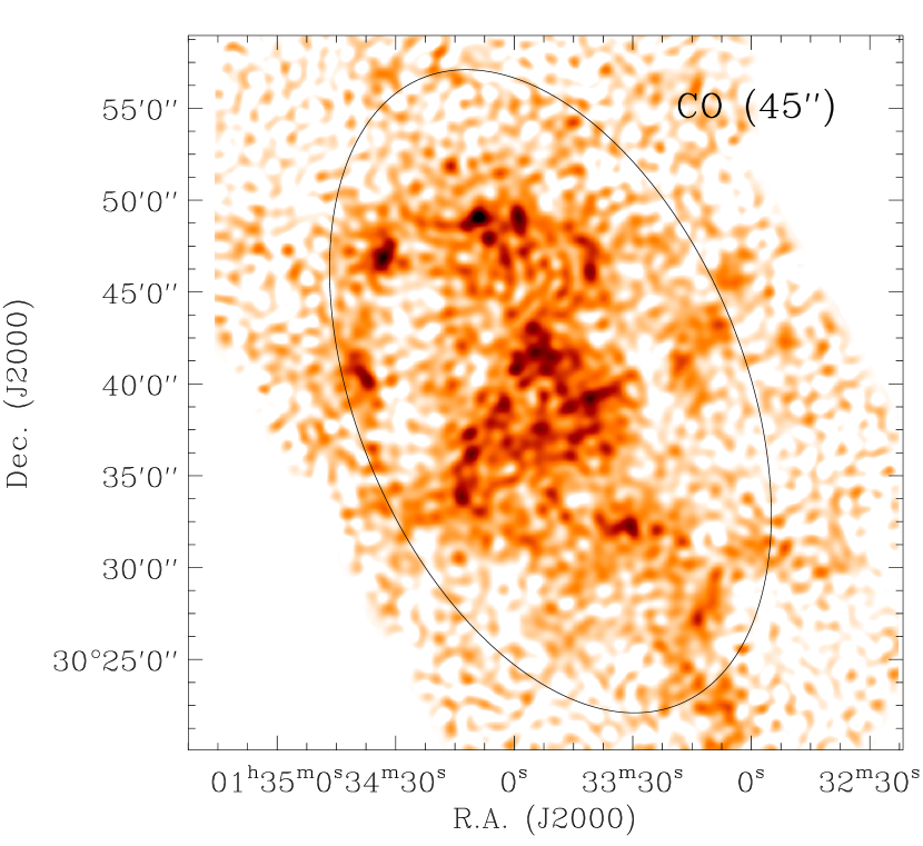
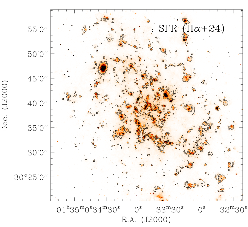
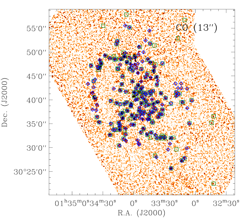
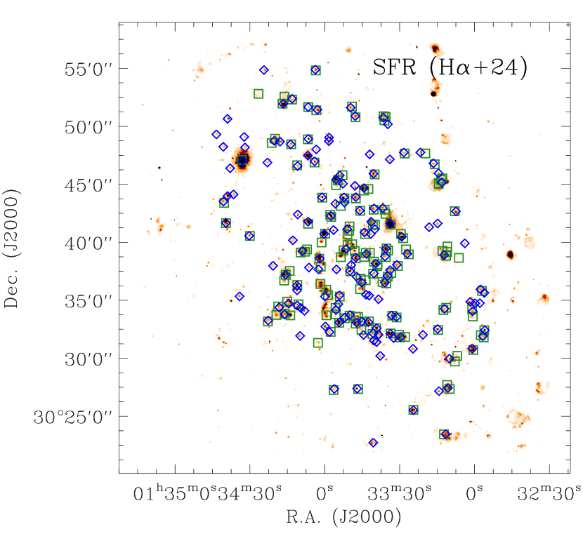
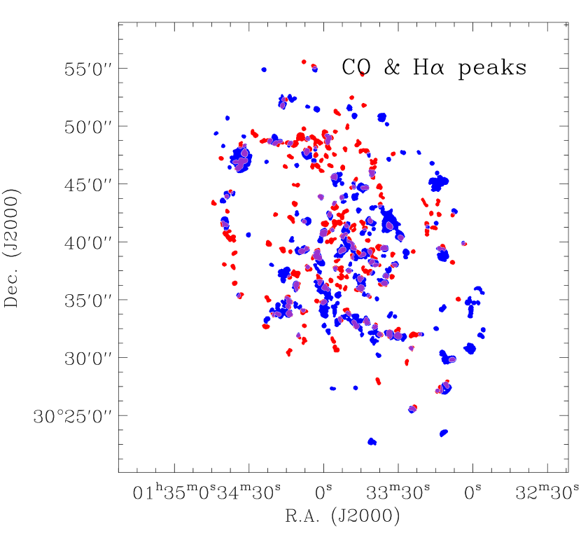
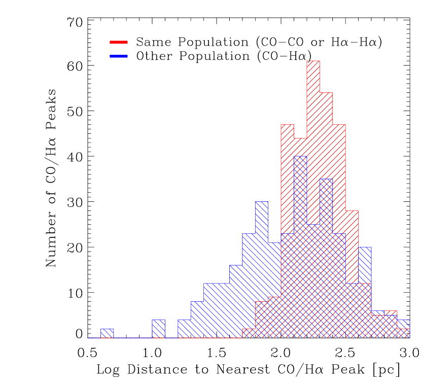
Figure 1.— CO and recent star formation in M33. Top left: Masked, integrated CO intensity smoothed to $\sim$$45\arcsec$ resolution to enhance the SNR. The black ellipse shows $R_{\rm gal}=4.5$ kpc ($\sim$$0.6~{}r_{25}$); we carry out our analysis inside this radius. Top right: H$\alpha$ emission corrected for extinction via combination with mid-IR emission. A black contour outlines regions that remain after the subtraction of the diffuse ionized gas (see text). Middle left: Positions of our CO peaks (blue diamonds) plotted on the full resolution CO map along with the cataloged positions of GMCs from Rosolowsky et al. (2007, green squares). Middle Right: Positions of our H$\alpha$ peaks (blue diamonds) along with the $150$ most luminous H II regions cataloged by Hodge et al. (2002, green squares). Bottom left: Relative distributions of bright CO (red) and H$\alpha$ (blue) emission and the area of overlap (purple), inflated by $6$″ for display reasons. Bottom right: Histograms of distance from each peak to the nearest peak of the same type (red, i.e., H$\alpha$ to H$\alpha$ or CO to CO) and of the other type (blue, CO to H$\alpha$ and vice versa).

Star-forming clouds consist mainly of H₂, which cannot be directly observed under typical conditions. Instead, H₂ is usually traced via emission from the second most common molecule, CO. We follow this approach, estimating H₂ masses from the CO $J=1-0$ data of Rosolowsky et al. (2007), which combines the BIMA (interferometric) data of Engargiola et al. (2003) and the FCRAO $14$ m (single-dish) data of Heyer et al. (2004). The resolution of the merged data cube is $13\arcsec\times 2.03$ km s^-1 with a median $1\sigma$ noise of $240$ mK ($\sim$$2.1$ M_⊙ pc^-2 for our adopted $X_{\rm CO}$). Rosolowsky et al. (2007) showed that this combined cube recovers the flux of the Heyer et al. (2004) FCRAO data.

We convert integrated CO intensities into molecular gas surface densities assuming $X_{\rm CO}$= $2.0\times 10^{20}$ cm^-2 (K km s^-1)^-1. This is approximately the Milky Way conversion factor and agrees well with work on M33 by Rosolowsky et al. (2003). For this $X_{\rm CO}$:

$$\Sigma_{\rm H2}\left[{\rm M}_{\odot}~{}{\rm pc}^{-2}\right]=4.4~{}I_{\rm CO}\left[{\rm K}~{}{\rm km~{}s}^{-1}\right]~{},$$ (1)

where $I_{\rm CO}$ is the integrated CO intensity over the line of sight and $\Sigma_{\rm H2}$ is the mass surface density of molecular gas, including helium.

The data cover a wide bandpass, only a small portion of which contains the CO line. As a result, direct integration of the cube over all velocities produces an unnecessarily noisy map. Therefore, we “mask” the data, identifying the velocity range likely to contain the CO line along each line of sight. We integrate over all channels with $\pm 25$ km s^-1 of the local mean H I velocity (using the data from Deul & van der Hulst, 1987). To ensure that this does not miss any significant emission, we also convolve the original CO cube to $30$″ resolution and then identify all regions above $3\sigma$ in $2$ consecutive channels. Any region within or near such a region is also included in the mask. We blank all parts of the data cube that do not meet either criteria and then integrate along the velocity axis to produce an integrated CO intensity map. Figure 1 shows this map at full resolution (middle left) and smoothed to $\sim$$45\arcsec$ resolution (top left) to increase the SNR and highlight extended emission. The noise in the integrated intensity map varies with position but typical $1\sigma$ values are $8-10$ M_⊙ pc^-2; the dynamic range (peak SNR) is $\sim$$20$. The $3\sigma$ mass sensitivity in an individual resolution element is $\sim$$10^{5}$ M_☉.

2.2. Recent Star Formation from H$\alpha$ and IR Data

We trace the distribution of recent star formation using H$\alpha$ emission, which is driven by ionizing photons produced almost exclusively in very young (massive) stars. We account for extinction by combining H$\alpha$ and infrared (24$\mu$m) emission, a powerful technique demonstrated by Calzetti et al. (2007) and Kennicutt et al. (2007, 2009). Assuming continuous star formation over the past $100$ Myr and studying a set of extragalactic star-forming regions, Calzetti et al. (2007) found the recent star formation rate (SFR) to be

$${\rm SFR}\left[{\rm M}_{\odot}~{}{\rm yr}^{-1}\right]=5.3\times 10^{-42}\left[L\left({\rm H}\alpha\right)+0.031\ L\left(24\mu{\rm m}\right)\right]~{},$$ (2)

where $L$(H$\alpha$) and $L(24\mu{\rm m})=\nu L_{\nu}(24\mu{\rm m})$ are the luminosities of a region in H$\alpha$ emission and at $24$µm, measured in erg s^-1.

The assumption of continuous star formation is certainly inapplicable to individual regions, which are better described by instantaneous bursts (e.g., Relaño & Kennicutt, 2009). We only report averages of a large set ($\sim$$150$) of regions, which together constitute a large part of M33’s total H$\alpha$, and argue that this justifies the application of Equation 2 (see Section 3.2). In any case SFR units allow ready comparison to previous work.

2.2.1 H$\alpha$ Data

We use the narrow-band H$\alpha$ image obtained by Greenawalt (1998) with the KPNO $0.6$ m telescope. The reduction, continuum subtraction, and other details of these data are described by Hoopes & Walterbos (2000). Before combination with the IR map, we correct the H$\alpha$ map for Galactic extinction using a reddening of $\mbox{E(B-V)}=0.042$ (Schlegel et al., 1998) and a ratio of H$\alpha$ narrow band extinction to reddening of $\mbox{R(\mbox{\rm H$\alpha$})}=2.33$.

Studies of M33 and other nearby galaxies find typically $\sim$$40$% of the H$\alpha$ emission to come from “diffuse ionized gas” (DIG, Hoopes & Walterbos, 2000; Thilker et al., 2002; Hoopes & Walterbos, 2003; Thilker et al., 2005). The origin of this emission is still debated; it may be powered by leaked photons from bright H II regions or it may arise “in situ” from isolated massive stars. We choose to remove this diffuse component from the H$\alpha$ map and any discussion of H$\alpha$ emission in the following analysis refers to this DIG-subtracted map (we assess the impact of this step in the Appendix). We do so using the following method from Greenawalt (1998). We begin by median filtering the H$\alpha$ map with a $900$ pc kernel. We then identify H II regions as areas in the original map that exceed the median-filtered map by an emission measure of $50$ pc cm^-6 (outlined by black contours in the top right panel of Figure 1). We blank these regions in the original map and smooth to get an estimate of DIG emission towards the H II regions. Our working map consists of only emission from the H II regions after the DIG foreground has been subtracted. The integrated H$\alpha$ flux (inside $R_{\rm gal}=4.5$ kpc) allocated to the diffuse map is $1.05\times 10^{40}$ erg s^-1 ($44$%) while the part allocated to the DIG-subtracted, H II-region map is $1.35\times 10^{40}$ erg s^-1 ($56$%), in good agreement with previous results on M33 and other nearby galaxies.

2.2.2 IR Data

We measure IR intensities from $24$ µm maps obtained by the Spitzer Space Telescope (PI: Gehrz et al. 2005, see also Verley et al. 2007). The data were reduced by K. Gordon (2009, private communication) following Gordon et al. (2005). Spitzer’s point spread function at $24$ µm is $\sim$$6$″, well below our smallest aperture size ($\sim$$18$″) and so is not a large concern.

As with the H$\alpha$ image, the $24$ µm map includes a substantial fraction of diffuse emission — infrared cirrus heated by an older population, emission from low-mass star-forming regions, and dust heated leakage from nearby H II regions, with a minor contribution from photospheric emission of old stars. Verley et al. (2007) argue that this diffuse emission accounts for $\sim$$2/3$ of all $24$ µm emission in M33. To isolate $24$ µm emission originating directly from H II regions, we follow a similar approach to that used to remove DIG from the H$\alpha$ map. The key difference is that instead of trying to identify all $24$ µm bright sources by filtering and applying a cut-off to the $24$ µm emission, we use the existing locations of H II regions to isolate any local $24$ µm excess associated with H II regions. We extinction-correct the DIG-subtracted H$\alpha$ emission using only this local excess in $24$ µm emission. The total integrated flux at $24$ µm ($R_{\rm gal}\leq 4.5$ kpc) is $3.92\times 10^{41}$ erg s^-1, the fraction of DIG-subtraced $24$ µm inside the H II region mask is $1.63\times 10^{41}$ erg s^-1 ($42$%). The the $24$ µm correction implies H$\alpha$ extinctions of $A_{\rm H\alpha}\sim 0.3-0.4$ magnitudes.

3. Methodology

To quantify the scale-dependence of the molecular star formation law, we measure the H₂ depletion time, $\tau_{\rm dep}=\mbox{$\Sigma_{\rm H2}$}/\mbox{$\Sigma_{\rm SFR}$}$, for apertures centered on bright CO and H$\alpha$ peaks. We treat the two types of peaks separately and vary the sizes of the apertures used. In this way we simulate a continuum of observations ranging from nearly an entire galaxy ( $>1$ kpc apertures) to studies of (almost) individual GMCs or H II regions ($75$ pc apertures). The CO data limit this analysis to galactocentric radius $<4.5$ kpc ($\sim$$0.6$ r₂₅).

3.1. Identifying CO and H$\alpha$ Peaks

We employ a simple algorithm to identify bright regions in the DIG-subtracted, extinction-corrected H$\alpha$ map and the integrated CO intensity map. This automated approach allows us to use the same technique on both maps to find peaks matched in scale to our smallest aperture ($75$ pc). It is also easily reproducible and extensible to other galaxies.

This algorithm operates as follows: We identify all contiguous regions above a certain intensity — the local $3\sigma$ in the CO map and $\sim$$1.9\times 10^{40}$ erg s^-1 kpc^-2 in the corrected H$\alpha$ map ($\sim$$0.1$ M_⊙ yr^-1 kpc^-2 following Equation 2). We reject small regions (area less than $\sim$$110$ arcsec², which correspond to $\sim$$1800$ pc² at the distance of M33) as potentially spurious; the remaining regions are expanded by $20$″ ($\sim$$80$ pc) in radius to include any low intensity envelopes. The positions on which we center our apertures are then the intensity-weighted average position of each distinct region.

We find $172$ CO regions and $154$ H$\alpha$ regions. Strictly speaking, these are discrete, significant emission features at $\sim$$50$ pc resolution. At this resolution, there is a close but not perfect match between these peaks and the real physical structures in the two maps — GMCs and H II regions. Figure 1 (middle panels) shows our peaks along with the cataloged positions of GMCs (Rosolowsky et al., 2007) and H II regions (Hodge et al., 2002). There is a good correspondence, with $>80\%$ of the $149$ known GMCs and the 150 brightest H II regions lying within $\sim$$6$″ (3 pixels) of one of our regions.

3.2. Measuring Depletion Times

For a series of scales $d$, we center an aperture of diameter $d$ on each CO and H$\alpha$ peak and then measure fluxes within that aperture to obtain a mass of H₂ ($M_{\rm H2}$) and a star formation rate (SFR). We then compute the median H₂ depletion time for the whole set of apertures. We do this for scales $d=1200$, $600$, $300$, $150$ and $75$ pc and record results separately for apertures centered on CO and H$\alpha$ peaks.

At larger spatial scales, apertures centered on different peaks overlap (because the average spacing between CO and H$\alpha$ peaks is less than the aperture size). To account for this, we measure only a subset of apertures chosen so that at least $80$% of the selected area belongs only to one aperture targeting a given peak type (CO or H$\alpha$) at one time.

While we center on particular peaks, we integrate over all emission in our maps within the aperture. At the smallest scales we probe ($75$ pc), this emission will arise mostly — but not exclusively — from the target region. At progressively larger scales, we will integrate over an increasing number of other regions.

Table 1$\tau_{\rm dep}$ as Function of Peak and Scale

Scale	Depletion Time (Gyr)
(pc)	centered on CO	centered on H$\alpha$	$\left<N\right>$
1200	$1.1\pm 0.1$	$0.9\pm 0.1$	16.2
600	$1.2\pm 0.3$	$1.0\pm 0.1$	5.2
300	$2.5\pm 0.5$	$0.64\pm 0.05$	2.1
150	$4.9\pm 0.9$	$0.41\pm 0.04$	1.4
75	$8.6\pm 2.1$	$0.25\pm 0.02$	1.1

3.3. Uncertainties

We estimate the uncertainty in our measurements using a Monte-Carlo analysis. For the high-SNR H$\alpha$ and $24$ µm maps, we add realistic noise maps to the observed “true” maps and repeat the identification and removal of DIG emission using smoothing kernels and emission measure cuts perturbed from the values in Section 2.2.1 by $\pm 25$%. The low SNR of the CO data requires a more complex analysis. We assume that all regions with surface densities above $10$ M_⊙ pc^-2 ($\sim$$1.5$ $\sigma$) in the integrated CO map contain true signal. We generate a noise map correlated on the ($13\arcsec$) spatial scale of our CO data and scale this noise map according to the square root of the number of channels along each line of sight in our masked CO cube (typically $5-7$). Then we add all emission from the pixels above $10$ M_⊙ pc^-2. Finally, we re-identify peaks in the new maps and re-measure $M_{\rm H2}$ and SFR in each region. We repeat this process $100$ times; the scatter in $\tau_{\rm dep}$ across these repetitions is our uncertainty estimate.

4. Results

Figure 2 shows a well-known result for M33. There is a strong correlation (rank correlation coefficient of $r\approx 0.8$) between the surface densities of SFR and H₂ at 1200 pc scales. Power law fits to the different samples (types of peaks) and Monte Carlo iterations yield H₂ depletion times, $\tau_{\rm dep}=M_{\rm H2}/{\rm SFR}$, of $\sim$$1$ Gyr (at H₂ surface densities of $3$ M_⊙ pc^-2) and power law indices of $\sim$$1.1-1.5$. These results (modulo some renormalization due to different assumptions) match those of Heyer et al. (2004) and Verley et al. (2010) in their studies of the star formation law in M33. The important point here is that there is good evidence for an internal H₂-SFR surface density relation in M33.

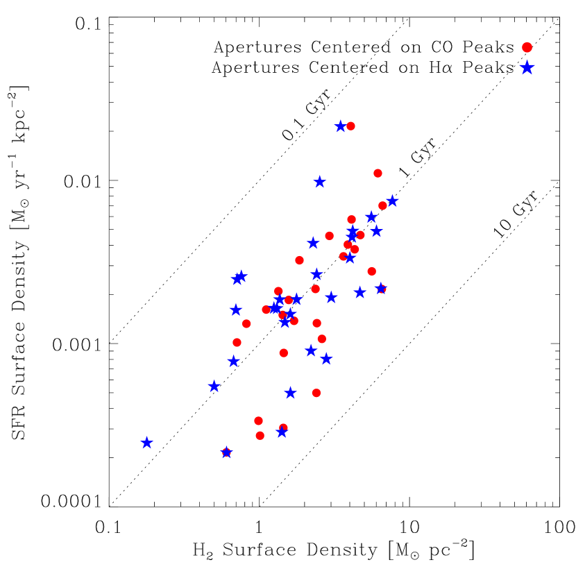
Figure 2.— The relationship between SFR surface density ($y$-axis) and H₂ surface density ($x$-axis) at large spatial scales. Red points show measurements integrated over (one independent subset of) 1200 pc apertures centered on CO peaks. Blue points show similar measurements centered on H$\alpha$ peaks. Dashed lines indicate fixed H₂ depletion times ranging from $0.1$ Gyr in the upper left to $10$ Gyr in the lower right.

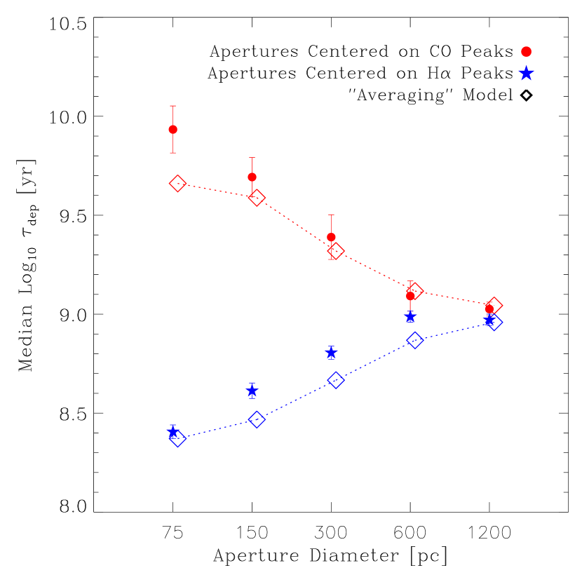
Figure 3.— Scale dependence of the H₂ depletion time, $\tau_{\rm dep}$, in M33. The $y$-axis shows the logarithm of the median H₂ depletion time for apertures of different diameters ($x$-axis) centered on CO peaks (red) and H$\alpha$ peaks (blue). Error bars correspond to uncertainty in the median estimated via a Monte-Carlo analysis. Dashed lines show expectation for simply averaging together two populations of regions in different states (Section 5).

We plot the median $\tau_{\rm dep}$ as a function of scale (aperture size) in Figure 3, giving results for apertures centered on CO (red circles) and H$\alpha$ (blue stars) peaks seperately. For the largest scales, we find a similar $\tau_{\rm dep}$ for both sets of apertures (as was evident from Figure 2). Going to smaller aperture sizes, $\tau_{\rm dep}$ becomes a strong function of scale and type of peak targeted. Small apertures centered on CO peaks have very long $\tau_{\rm dep}$ (up to 10 Gyr). Small apertures targeted toward H$\alpha$ peaks have very short $\tau_{\rm dep}$ ($0.3$ Gyr). This may not be surprising, given the expectations that we outlined in Section 1 and the distinctness of the bright H$\alpha$ and CO distributions seen in the lower left panel of Figure 1, but the dramatic difference as one goes from $\sim$kpc to $\sim$$100$ pc scales is nonetheless striking.

A few caveats apply to Figure 3. First, in subtracting the diffuse emission (DIG) from the H$\alpha$ map, we removed $\sim$$40\%$ of the flux. This could easily include faint regions associated with CO peaks, which instead show up as zeros in our map. Perhaps more importantly, we use the $24$ µm map only to correct the DIG-subtraced H$\alpha$ map for extinction. Any completely embedded star formation will therefore be missed. For both of these reasons, the SFR associated with the red points, while it represents our best guess, may be biased somewhat low and certainly reflects emission from relatively evolved regions — those regions that have H$\alpha$ fluxes above our DIG-cutoff value. There is no similar effect for the CO map.

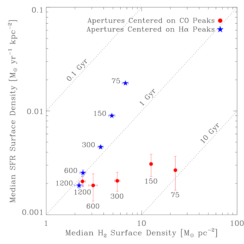
Figure 4.— Scale dependence of the location of data in the star formation law parameter space. Red points show the median $\Sigma_{\rm SFR}$ ($y$-axis) and $\Sigma_{\rm H2}$ ($x$-axis) for apertures centered on CO peaks. Blue stars show the same for apertures centered on H$\alpha$ peaks. Dashed lines as in Figure 2.

Figure 3 implies that there is substantial movement of points in the star formation law parameter space as we zoom in to higher resolution on one set of peaks or another. Figure 4 shows this behavior, plotting the median $\Sigma_{\rm SFR}$ and median $\Sigma_{\rm H2}$ for each set of apertures (N.B., the ratio of median $\Sigma_{\rm H2}$ to median $\Sigma_{\rm SFR}$ does not have to be identical to the median $\tau_{\rm dep}$; the difference is usually $\lesssim 30\%$). We plot only medians because individual data are extremely uncertain, include many upper limits, and because we are primarily interested in the systematic effects of resolution on data in this parameter space.

Apertures centered on CO peaks (red points) have approximately constant $\Sigma_{\rm SFR}$, regardless of resolution. This can be explained if emission in the H$\alpha$ map is homogeneously distributed as compared to the position of CO peaks. Meanwhile there is a strong change in $\Sigma_{\rm H2}$ for decreasing aperture sizes on the same peaks; $\Sigma_{\rm H2}$ goes up as the bright region fills more and more of the aperture. A similar effect can be seen for the H$\alpha$ (blue stars), though there is more evolution in $\Sigma_{\rm H2}$ with increasing resolution because most bright H$\alpha$ regions also show some excess in CO emission.

5. Discussion

Figure 3 shows that by zooming in on an individual star-forming region, one loses the ability to recover the star formation law observed on large scales. For apertures $\lesssim 300$ pc in size, the relative amounts of CO emission and H$\alpha$ intensity vary systematically as a function of scale and what type of region one focuses on. Another simple way to put this, demonstrated in Figure 4, is that scatter orthogonal to the SFR-H₂ relation increases with increasing resolution. Eventually this washes out the scaling seen on large scales and the star formation law may be said to “break down”.

What is the origin of this scale dependence? In principle one can imagine at least six sources of scale dependence in the star formation law:

1. Statistical fluctuations due to noise in the maps.

2. Feedback effects of stars on their parent clouds.

3. Drift of young stars from their parent clouds.

4. Region-to-region variations in the efficiency of star formation.

5. Time-evolution of individual regions.

6. Region-to-region variations in how observables map to physical quantities.

Our observations are unlikely to be driven by any of the first three effects. In principle, statistical fluctuations could drive the identification of H$\alpha$ and CO peaks leading to a signal similar to Figure 3 purely from noise. However, our Monte Carlo calculations, the overall SNR in the maps, and the match to previous region identifications make it clear that this is not the case.

Photoionization by young stars can produce CO shells around H II regions inside of a larger cloud or complex. This is a clear case of a small-scale offset between H$\alpha$ and CO. However, the physical scales in Figure 3 are too large for this effect to have much impact, it should occur on scales more like $\sim$$10$ pc.

Similarly, the scales over which $\tau_{\rm dep}$ diverges between CO and H$\alpha$ peaks ($75-300$ pc) are probably too large to be produced by drift between young stars and their parent cloud. A typical internal GMC velocity dispersion in M33 is a few km s^-1 ($1\sigma$; Rosolowsky et al., 2003). Over an average cloud lifetime ($\sim$$30$ Myr; Blitz et al., 2007; Kawamura et al., 2009), this implies a drift of at most $100$ pc. This extreme case is just large enough to register in our plot but unlikely to drive the signal we see at scales of $150-300$ pc. See Engargiola et al. (2003) for a similar consideration of GMCs and H I filaments.

Instead of drifts or offsets, what we observe is simply a lack of direct correspondence between the CO and H$\alpha$ luminosities of individual star-forming regions. The brightest $150$ CO peaks are simply not identical to the brightest $150$ H$\alpha$ peaks. The bottom right panel of Figure 1 shows this clearly; about a third of the peaks in M33 are nearer to another peak of their own type (i.e., CO to CO or H$\alpha$ to H$\alpha$) than to a peak of the other type. Thus Figure 3 shows that the ratio of CO to H$\alpha$ emission varies dramatically among star-forming regions. In this case the size scale on the $x$-axis in Figure 3 is actually a proxy for the number of regions inside the aperture. In M33, apertures of $75$ pc diameter usually contain a single peak. At $150$ pc, this is still the case $\sim$$70\%$ of the time, and at $300$ pc only a few regions are included in each aperture.

Why does the ratio of CO-to-H$\alpha$ vary so strongly from region-to-region? The efficiency with which gas form stars may vary systematically from region to region (with high H$\alpha$ peaks being high-efficiency regions), star-forming regions may undergo dramatic changes in their properties as they evolve (with H$\alpha$ peaks being evolved regions), or the mapping of observables to physical quantities (Equations 1 and 2) may vary from region to region.

It is difficult to rule out region-to-region efficiency variations, but there is also no strong evidence for them. Leroy et al. (2008) looked for systematic variations in $\tau_{\rm dep}$ as a function of a number of environmental factors and found little evidence for any systematic trends. Krumholz & McKee (2005); Krumholz & Tan (2007) suggested that the cloud free-fall time determines $\tau_{\rm dep}$ to first order, but based on Rosolowsky et al. (2003), the dynamic range in free-fall times for M33 clouds is low. On the other hand, Gardan et al. (2007) found unusually low values of $\tau_{\rm dep}$ in the outer disk of M33.

There is strong evidence for evolution of star-forming regions. Fukui et al. (1999), Blitz et al. (2007), Kawamura et al. (2009), and Chen et al. (2010) showed that in the LMC, the amount of H$\alpha$ and young stars associated with a GMC evolves significantly across its lifetime. In our opinion this is the most likely explanation for the behavior in Figure 3. Star-forming regions undergo a very strong evolution from quiescent cloud, to cloud being destroyed by H II region, to exposed cluster or association. When an aperture contains only a few regions, $\tau_{\rm dep}$ for that aperture will be set by the evolutionary state of the regions inside it. That state will in turn determine whether the aperture is identified as a CO peak or an H$\alpha$ peak. CO peaks will preferentially select sites of heavily embedded or future star formation while H$\alpha$ peaks are relatively old regions that formed massive stars a few Myr ago.

Region-to-region variations in the mapping of observables (CO and H$\alpha$) to physical quantities (H₂ mass and SFR) are expected. Let us assume for the moment that the ratio of H₂ to SFR is constant and independent of scale. Then to explain the strong scale dependence of the ratio of CO to H$\alpha$ in Figure 3 there would need to be much more H₂ per unit CO near H$\alpha$ peaks and many more recently formed stars per ionizing photon near the CO peaks. At least some of these effects have been claimed: e.g., Israel (1997) find a strong dependence of $X_{\rm CO}$ on radiation field and Verley et al. (2010) suggest that incomplete sampling of the IMF in regions with low SFRs drive the differences they observe between star formation tracers. However, both claims are controversial and it seems very contrived to invoke a scenario where only this effect drives the breakdown in Figure 3. It seems more plausible that the mapping of observables to physical quantities represents a secondary source of scatter correlated with the evolutionary state of a region (e.g., the age of the stellar population).

5.1. Comparison to a Simple Model

We argue that the behavior seen in Figures 3 and 4 comes from averaging together regions in different states. Here we implement a simple model to demonstrate that such an effect can reproduce the observed behavior.

The model is as follows: we consider a population of regions. We randomly assign each region to be an “H$\alpha$ peak” or a “CO peak” with equal chance of each. CO peaks have $5$ times as much CO as H$\alpha$ and H$\alpha$ peaks have $5$ times as much H$\alpha$ as CO (roughly driven by the difference between the results for $75$ pc apertures in Table 1). Physically, the idea is simply to build a population of regions that is an equal mix “young” (high CO-to-H$\alpha$) and “old” (low CO-to-H$\alpha$). Dropping an aperture to contain only a young (CO peak) or old (H$\alpha$ peak) region will recover our results at $75$ pc scales by construction. Next we average each of our original region with another, new region (again randomly determined to be either a CO or H$\alpha$ peak). We add the CO and H$\alpha$ emission of the two region together, record the results. We then add a third region (again randomly young or old), and so on.

The result is a prediction for the ratio of CO to H$\alpha$ as a function of two quantities: 1) the number of regions added together and 2) the type of the first region (CO or H$\alpha$ peak). Using the average number of regions per aperture listed in Table 1 and normalizing to an average depletion time of 1 Gyr, we then have a prediction for $\tau_{\rm dep}$ as a function of scale. This appears as the diamond symbols and dashed lines in Figure 3.

Given the simplicity of the model, the agreement between observations and model in Figure 3 is good. Our observations can apparently be explained largely as the result of averaging together star-forming regions in distinct evolutionary states. At scales where a single region dominates, the observed $\tau_{\rm dep}$ is a function of the state of that region. As more regions are included, $\tau_{\rm dep}$ just approaches the median value for the system.

5.2. $\tau_{\rm dep}$ vs. Scale at Different Radii

The star formation law apparently breaks down (or at least includes a large amount of scatter) on scales where one resolution element corresponds to an individual star-forming region. The spatial resolution at which this occurs will vary from system to system according to the space density of star-forming regions in the system.

The surface densities of star formation and H₂ vary with radius in M33 (Heyer et al., 2004). This allows us to break the galaxy into two regions, a high surface density inner part ($r_{\rm gal}=0-2.2$ kpc) and a low surface density outer part ( $r_{\rm gal}=2.2-4.5$ kpc). We measure the scale dependence of $\tau_{\rm dep}$ for each region in the same way that we did for all data. An important caveat is that the DIG subtraction becomes problematic for the outer region, removing a number of apparently real but low-brightness H II regions from the map. We achieve the best results for large radii with the DIG subtraction is turned off and report those numbers here. The basic result of a larger-scale of divergence in the outer disk remains the same with the DIG subtraction on or off.

We find the expected result, that $\tau_{\rm dep}$ for CO and H$\alpha$ peaks diverges at larger spatial scales in the outer disk than the inner disk. In both cases the ratio of $\tau_{\rm dep}$ at CO peaks to $\tau_{\rm dep}$ at H$\alpha$ peaks is $\sim$$1$ for $1200$ pc apertures. For $600$ pc apertures that ratio remains $\sim$$1$ in the inner disk but climbs to $\sim$$2$ in the outer disk, suggesting that by this time there is already some breakdown in the SFR-H₂ relation. For $300$ pc apertures, the same ratio is $\sim$$1.7$ in the inner disk and $\sim$$3$ in the outer disk. It thus appears that at large radii in M33 the star formation law breaks down on scales about twice that of the inner disk, though the need to treat the DIG inhomogeneously means that this comparison should not be overinterpreted.

6. Conclusions

Our main conclusion is that the molecular star formation law observed in M33 at large scales (e.g., Heyer et al., 2004; Verley et al., 2010) shows substantial scale dependence if one focuses on either CO or H$\alpha$ peaks. The median depletion time (or CO-to-H$\alpha$ ratio) measured in a $75$ pc diameter aperture (derived from averaging $\sim$$150$ such apertures) varies by more than an order of magnitude between CO and H$\alpha$ peaks. At large ($\sim$kpc) scales this difference mostly vanishes. We argue that the scale for the breakdown is set by the spatial separation of high-mass star-forming regions, with the breakdown occurring when an aperture includes only a few such regions in specific evolutionary states (a scale that corresponds to $\sim$$300$ pc in M33).

In this case the scaling relation between gas and star formation rate surface density observed at large scales does not have its direct origin in an instantaneous cloud-scale relation. Individual GMCs and H II regions will exhibit a CO-to-H$\alpha$ ratio that depends on their evolutionary state (likely with significant additional stochasticity) and as a result the $\sim$$150$ brightest objects at a given wavelength will be a function of what evolutionary state that observation probes. This divergence is consistent with recent results from the LMC (Kawamura et al., 2009) indicating that individual GMCs exhibit a range of evolutionary states over their $20-30$ Myr lifetime.

This does not mean that comparisons of tracers of recent and future star formation on small scales are useless. To the contrary, such observations contain critical information about the evolution of individual clouds as a function of time and location that is washed out at large scales ($\gtrsim 300$ pc in M33). However, once one moves into the regime where a single object contributes heavily to each measurement, it is critical to interpret the results in light of the evolution of individual clouds.

Here we test how our method of selecting peaks and the removal of a diffuse ionized component affect our results.

First, we repeating the analysis on the original maps without any DIG subtraction. We show the results in the left panel of Figure 5, along with the original measurements (in gray) from Figure 3. To first order, the scale-dependence of $\tau_{\rm dep}$ is unchanged, but the H₂ depletion are offset; $\tau_{\rm dep}$ derived from maps with no DIG subtraction is a factor of $\sim$$2$ smaller from the DIG-subtracted maps.

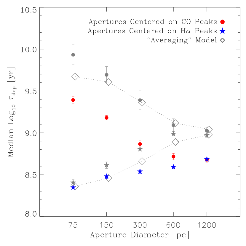
Figure 5.— Tests of systematics. We repeat the measurement of $\tau_{\rm dep}$ and remake Figure 3 varying our methodology. Left: Results if we perform no DIG-subtraction on the H$\alpha$ maps. Right: Results if we use the known positions of GMCs and H II regions from Rosolowsky et al. (2007) and Hodge et al. (2002). In both panels, our original results using the DIG-subtracted maps and an automated peak finder appear as gray points. Our qualitative conclusions are largely robust to these changes in methodology, though the overall normalization of CO-to-H$\alpha$ ratio does depend on the DIG subtraction.

As a second test we assess the impact of the particular choice of aperture positions. In main text we used a peak-finding algorithm. Here we test the effect of using published positions of GMCs and H II regions instead. The right panel in Figure 5 shows our original data in gray while the red and blue points are $\tau_{\rm dep}$ derived using the Rosolowsky et al. (2007) and Hodge et al. (2002) catalogs. The median $\tau_{\rm dep}$ at large scale is unchanged from Figure 3 (gray values). However, for apertures centered on GMCs, $\tau_{\rm dep}$ on small scales does change from our analysis. This difference originates in different numbers and locations of the positions that are studied. In our original analysis, we study $172$ positions which have CO emission peaks above $3\sigma$. The Rosolowsky catalog, on the other hand, consists of only $140$ positions inside a galactocentric radius of $4.5$ kpc. In addition, a subset of the two samples targets different regions in M33: First, the catalog positions tend to be more clustered than the “peak” positions which leads to a somewhat larger number ($5-15\%$) of objects in the smaller apertures and a smaller deviation in depletion times for CO or H II centered apertures. Second, while the molecular gas surface densities at the positions of the two samples do not differ significantly, the star formation rate surface densities are a factor of $\sim$$3$ higher for the catalog positions as compared to the (more numerous) “peak” positions. This leads to shorter H₂ depletion times on small scales for the catalog sample.

Both tests show that the analyzed scale dependence of the star formation relation and the determination of its origin is not strongly dependent on the particular methodology chosen in this paper. While global shifts in the derived depletion times can arise due to the subtraction of diffuse H$\alpha$ emission, we find only small variations in the scale dependence due to different selection of positions where we perform our study.

References

- Bigiel et al. (2008) Bigiel, F., Leroy, A., Walter, F., Brinks, E., de Blok, W. J. G., Madore, B., & Thornley, M. D. 2008, AJ, 136, 2846
- Blitz et al. (2007) Blitz, L., Fukui, Y., Kawamura, A., Leroy, A., Mizuno, N., & Rosolowsky, E. 2007, Protostars and Planets V, 81
- Calzetti et al. (2007) Calzetti, D., Kennicutt, R. C., Engelbracht, C. W., Leitherer, C., Draine, B. T., Kewley, L., Moustakas, J., Sosey, M., Dale, D. A., Gordon, K. D., Helou, G. X., Hollenbach, D. J., Armus, L., Bendo, G., Bot, C., Buckalew, B., Jarrett, T., Li, A., Meyer, M., Murphy, E. J., Prescott, M., Regan, M. W., Rieke, G. H., Roussel, H., Sheth, K., Smith, J. D. T., Thornley, M. D., & Walter, F. 2007, ApJ, 666, 870
- Chen et al. (2010) Chen, C., Indebetouw, R., Chu, Y., Gruendl, R. A., Testor, G., Heitsch, F., Seale, J. P., Meixner, M., & Sewilo, M. 2010, ArXiv e-prints
- Deul & van der Hulst (1987) Deul, E. R., & van der Hulst, J. M. 1987, A&AS, 67, 509
- Engargiola et al. (2003) Engargiola, G., Plambeck, R. L., Rosolowsky, E., & Blitz, L. 2003, ApJS, 149, 343
- Evans et al. (2009) Evans, N. J., Dunham, M. M., Jørgensen, J. K., Enoch, M. L., Merín, B., van Dishoeck, E. F., Alcalá, J. M., Myers, P. C., Stapelfeldt, K. R., Huard, T. L., Allen, L. E., Harvey, P. M., van Kempen, T., Blake, G. A., Koerner, D. W., Mundy, L. G., Padgett, D. L., & Sargent, A. I. 2009, ApJS, 181, 321
- Fukui et al. (1999) Fukui, Y., Mizuno, N., Yamaguchi, R., Mizuno, A., Onishi, T., Ogawa, H., Yonekura, Y., Kawamura, A., Tachihara, K., Xiao, K., Yamaguchi, N., Hara, A., Hayakawa, T., Kato, S., Abe, R., Saito, H., Mano, S., Matsunaga, K., Mine, Y., Moriguchi, Y., Aoyama, H., Asayama, S., Yoshikawa, N., & Rubio, M. 1999, PASJ, 51, 745
- Gardan et al. (2007) Gardan, E., Braine, J., Schuster, K. F., Brouillet, N., & Sievers, A. 2007, A&A, 473, 91
- Gehrz et al. (2005) Gehrz, R. D., Polomski, E., Woodward, C. E., McQuinn, K., Boyer, M., Humphreys, R. M., Brandl, B., van Loon, J. T., Fazio, G., Willner, S. P., Barmby, P., Ashby, M., Pahre, M., Rieke, G., Gordon, K., Hinz, J., Engelbracht, C., Alonso-Herrero, A., Misselt, K., Pérez-González, P. G., & Roellig, T. 2005, in Bulletin of the American Astronomical Society, Vol. 37, Bulletin of the American Astronomical Society, 451–+
- Gordon et al. (2005) Gordon, K. D., Rieke, G. H., Engelbracht, C. W., Muzerolle, J., Stansberry, J. A., Misselt, K. A., Morrison, J. E., Cadien, J., Young, E. T., Dole, H., Kelly, D. M., Alonso-Herrero, A., Egami, E., Su, K. Y. L., Papovich, C., Smith, P. S., Hines, D. C., Rieke, M. J., Blaylock, M., Pérez-González, P. G., Le Floc’h, E., Hinz, J. L., Latter, W. B., Hesselroth, T., Frayer, D. T., Noriega-Crespo, A., Masci, F. J., Padgett, D. L., Smylie, M. P., & Haegel, N. M. 2005, PASP, 117, 503
- Greenawalt (1998) Greenawalt, B. E. 1998, PhD thesis, AA(New Mexico State University)
- Heyer et al. (2004) Heyer, M. H., Corbelli, E., Schneider, S. E., & Young, J. S. 2004, ApJ, 602, 723
- Hodge et al. (2002) Hodge, P. W., Skelton, B. P., & Ashizawa, J., eds. 2002, Astrophysics and Space Science Library, Vol. 221, An Atlas of Local Group Galaxies
- Hoopes & Walterbos (2000) Hoopes, C. G., & Walterbos, R. A. M. 2000, ApJ, 541, 597
- Hoopes & Walterbos (2003) —. 2003, ApJ, 586, 902
- Israel (1997) Israel, F. P. 1997, A&A, 328, 471
- Kawamura et al. (2009) Kawamura, A., Mizuno, Y., Minamidani, T., Filipović, M. D., Staveley-Smith, L., Kim, S., Mizuno, N., Onishi, T., Mizuno, A., & Fukui, Y. 2009, ApJS, 184, 1
- Kennicutt et al. (2009) Kennicutt, R. C., Hao, C., Calzetti, D., Moustakas, J., Dale, D. A., Bendo, G., Engelbracht, C. W., Johnson, B. D., & Lee, J. C. 2009, ApJ, 703, 1672
- Kennicutt (1998) Kennicutt, Jr., R. C. 1998, ARA&A, 36, 189
- Kennicutt et al. (2007) Kennicutt, Jr., R. C., Calzetti, D., Walter, F., Helou, G., Hollenbach, D. J., Armus, L., Bendo, G., Dale, D. A., Draine, B. T., Engelbracht, C. W., Gordon, K. D., Prescott, M. K. M., Regan, M. W., Thornley, M. D., Bot, C., Brinks, E., de Blok, E., de Mello, D., Meyer, M., Moustakas, J., Murphy, E. J., Sheth, K., & Smith, J. D. T. 2007, ApJ, 671, 333
- Krumholz & McKee (2005) Krumholz, M. R., & McKee, C. F. 2005, ApJ, 630, 250
- Krumholz & Tan (2007) Krumholz, M. R., & Tan, J. C. 2007, ApJ, 654, 304
- Leroy et al. (2008) Leroy, A. K., Walter, F., Brinks, E., Bigiel, F., de Blok, W. J. G., Madore, B., & Thornley, M. D. 2008, AJ, 136, 2782
- Murgia et al. (2002) Murgia, M., Crapsi, A., Moscadelli, L., & Gregorini, L. 2002, A&A, 385, 412
- Relaño & Kennicutt (2009) Relaño, M., & Kennicutt, R. C. 2009, ApJ, 699, 1125
- Rosolowsky et al. (2003) Rosolowsky, E., Engargiola, G., Plambeck, R., & Blitz, L. 2003, ApJ, 599, 258
- Rosolowsky et al. (2007) Rosolowsky, E., Keto, E., Matsushita, S., & Willner, S. P. 2007, ApJ, 661, 830
- Schlegel et al. (1998) Schlegel, D. J., Finkbeiner, D. P., & Davis, M. 1998, ApJ, 500, 525
- Schmidt (1959) Schmidt, M. 1959, ApJ, 129, 243
- Thilker et al. (2005) Thilker, D. A., Hoopes, C. G., Bianchi, L., Boissier, S., Rich, R. M., Seibert, M., Friedman, P. G., Rey, S.-C., Buat, V., Barlow, T. A., Byun, Y.-I., Donas, J., Forster, K., Heckman, T. M., Jelinsky, P. N., Lee, Y.-W., Madore, B. F., Malina, R. F., Martin, D. C., Milliard, B., Morrissey, P. F., Neff, S. G., Schiminovich, D., Siegmund, O. H. W., Small, T., Szalay, A. S., Welsh, B. Y., & Wyder, T. K. 2005, ApJ, 619, L67
- Thilker et al. (2002) Thilker, D. A., Walterbos, R. A. M., Braun, R., & Hoopes, C. G. 2002, AJ, 124, 3118
- Verley et al. (2010) Verley, S., Corbelli, E., Giovanardi, C., & Hunt, L. K. 2010, A&A, 510, A64+
- Verley et al. (2007) Verley, S., Hunt, L. K., Corbelli, E., & Giovanardi, C. 2007, A&A, 476, 1161
- Wilson et al. (2008) Wilson, C. D., Petitpas, G. R., Iono, D., Baker, A. J., Peck, A. B., Krips, M., Warren, B., Golding, J., Atkinson, A., Armus, L., Cox, T. J., Ho, P., Juvela, M., Matsushita, S., Mihos, J. C., Pihlstrom, Y., & Yun, M. S. 2008, ApJS, 178, 189
- Wong & Blitz (2002) Wong, T., & Blitz, L. 2002, ApJ, 569, 157