Additional Corrections to the Gross-Llewellyn Smith Sum Rule

Abstract

We investigate some QCD corrections that contribute to the Gross–Llewellyn Smith (GLS) sum rule, but have not been included in previous analyses of it. We first review the techniques by which the $xF_{3}$ structure function is extracted from combinations of neutrino and antineutrino cross sections. Next we investigate corrections to the GLS sum rule, with particular attention to contributions arising from strange quark distributions and from charge symmetry violating (CSV) parton distributions. We find that additional corrections from strange quarks and parton CSV are likely to have a small but potentially significant role in decreasing the current discrepancy between the experimental and theoretical estimates of the Gross Llewellyn Smith sum rule.

I Introduction

The Gross Llewellyn Smith (GLS) sum rule (sometimes referred to as the baryon sum rule) is obtained from an integral of the $xF_{3}$ structure function obtained in charged-current deep inelastic scattering (DIS) from neutrinos and antineutrinos on nucleon or nuclear targets GLS ; Hin96 . In recent years the most precise neutrino data has been obtained by the CCFR and NuTeV collaborations, from interactions of neutrinos and antineutrinos with an iron target Con98 . From measurements by the CCFR group CCFR , values have been obtained for the GLS sum rule. At the value $Q^{2}=3$ GeV², the CCFR analysis claimed a precision of roughly 3%. The CCFR data could also be used to obtain the GLS sum rule as a function of $Q^{2}$; this allows one to test contributions from higher-order QCD corrections larin and from higher-twist terms braun . The current status of various DIS sum rules has been summarized in a review article by Hinchliffe and Kwiatkowski Hin96 .

In this paper, we point out that some additional QCD effects, particularly contributions from strange quarks and parton charge symmetry violation (CSV), have not been included to date in estimates of the GLS sum rule. One now has recent experimental data on strange quark parton distributions, in particular on the asymmetry between strange and antistrange quarks, which is relevant for the GLS sum rule. In addition, there is much interest in the possibility of CSV in the parton distributions Londergan:2009kj ; Londergan:1998ai ; MRST03 ; Bentz:2009yy .

We examine the possible contributions of these terms to the Gross-Llewellyn Smith sum rule, finding that such corrections are likely to produce small but potentially significant effects. At present, theoretical estimates of the GLS sum rule lie one or two standard deviations below the data Hin96 . We point out that contributions from strange quarks and partonic CSV are likely to improve the agreement between theory and experiment.

Our paper is organized as follows. In Sect. II we review the form of neutrino cross sections and the derivation of the GLS sum rule. The experimental results of the CCFR group CCFR are summarized and compared with the theoretical calculations of Hinchliffe and Kwiatkowski Hin96 . In Sect. III we review how the structure functions, particularly $xF_{3}$, are extracted from experimental data. We pay special attention to contributions from strange quarks and partonic CSV. In Sect. IV, we make estimates of these contributions to the GLS sum rule.

In Sect. IV.4, we review isoscalar corrections to the data, which arise because iron is not an isoscalar target. Because of the way in which isoscalar corrections have been implemented in previous analyses, it is difficult for us to give a definitive, quantitative estimate of the contribution of strange quarks and partonic charge symmetry violation in the GLS sum rule. Nevertheless, our analysis clearly establishes that these corrections can be as large as the quoted errors on the GLS sum rule and that they tend to improve the agreement between theory and experiment. Our results show that these corrections should be included in future analyses.

II Neutrino Cross Sections and the Gross-Llewellyn Smith Sum Rule

The cross section for charged current (CC) interactions initiated by neutrinos or antineutrinos on nucleons on a proton is shown schematically in Fig. 1. It has the form Con98 ; Londergan:2009kj

$$\frac{d^{2}\sigma^{\nu(\bar{\nu})\,p}_{{\scriptscriptstyle CC}}}{dx\,dy} = \frac{{{G_{{\scriptscriptstyle F}}}^{2}}ME_{\nu}}{\pi}\bigl{[}f_{1}(y)F_{2}^{W^{\pm}p}(x,Q^{2})$$

$$\pm f_{2}(y)xF_{3}^{W^{\pm}p}(x,Q^{2})\bigr{]}\ ;$$

$$f_{1}(y) = 1-y-\frac{xyM^{2}}{s}+\frac{y^{2}}{2}\frac{1+4M^{2}x^{2}/Q^{2}}{1+R_{L}^{\nu}(x,Q^{2})}$$

$$\approx 1-y+\frac{y^{2}}{2(1+R_{L}^{\nu})}\ ;$$

$$f_{2}(y) = y-\frac{y^{2}}{2}\ .$$ (1)

The relativistic invariants in Eq. (1) are $Q^{2}=-q^{2}$, the square of the four momentum transfer for the reaction, $x$ and $y$. For four momentum $k$ ($p$) for the initial state lepton (nucleon), we have the relations

$$x={Q^{2}\over 2p\cdot q};\qquad y={p\cdot q\over p\cdot k};\qquad s=(k+p)^{2}\ .$$ (2)

Eq. (1) applies in the limit $Q^{2}<<{M_{{\scriptscriptstyle W}}^{2}}$. We have introduced the Fermi coupling constant, ${G_{{\scriptscriptstyle F}}}$, in terms of the electromagnetic coupling constant $\alpha$, the $W$ boson mass $M_{{\scriptscriptstyle W}}$, and the weak mixing angle $\theta_{{\scriptscriptstyle W}}$,

$${G_{{\scriptscriptstyle F}}}=\frac{\pi\alpha}{\sqrt{2}{\sin^{2}\theta_{{\scriptscriptstyle W}}}{M_{{\scriptscriptstyle W}}^{2}}}\ .$$ (3)

Figure 1: Schematic picture of charged-current amplitudes in DIS induced by neutrinos or antineutrinos.

For neutrino-induced interactions, $F_{2}^{W^{+}p}(x,Q^{2})$ represents the $F_{2}$ structure function corresponding to a $W^{+}$ being absorbed on the proton. In Eq. (1) we have written the structure function $F_{1}$ in terms of the structure function $F_{2}$ and the longitudinal to transverse cross section ratio $R_{L}^{\nu}$, i.e.

$$2x\,F_{1}^{W^{+}p}(x,Q^{2})=\frac{1+4M^{2}x^{2}/Q^{2}}{1+R^{\nu}_{L}(x,Q^{2})}F_{2}^{W^{+}p}(x,Q^{2}).$$ (4)

For the CC reactions initiated by neutrinos, the experimental values for $R^{\nu}_{L}$ are summarized in the review article by Conrad, Shaevitz and Bolton Con98 .

The most accurate neutrino and antineutrino cross sections are on nuclear targets, particularly (in the case of the CCFR and NuTeV measurements) on iron targets. The structure functions are typically described in terms of nuclear parton distributions. At sufficiently high values of $Q^{2}$, the structure functions per nucleon for a nucleus with $Z$ protons and $N=A-Z$ neutrons can be written in terms of averages and differences of structure functions for neutrinos and antineutrinos.

Therefore we define

$$\overline{F}_{2}^{WA}(x) = {\frac{Z}{2A}}\left(F_{2}^{W^{+}p}(x)+F_{2}^{W^{+}p}(x)\right)$$

$$+ {\frac{N}{2A}}\left(F_{2}^{W^{+}n}(x)+F_{2}^{W^{-}n}(x)\right)\ ;$$

$$x\overline{F}_{3}^{WA}(x) = {\frac{Z}{2A}}\left(xF_{3}^{W^{+}p}(x)+xF_{3}^{W^{-}p}(x)\right)$$

$$+ {\frac{N}{2A}}\left(xF_{3}^{W^{+}n}(x)+xF_{3}^{W^{-}n}(x)\right)\ ;$$

$$\Delta F_{2}^{WA}(x) = {\frac{Z}{A}}(F_{2}^{W^{+}p}(x)-F_{2}^{W^{-}p}(x))$$

$$+ {\frac{N}{A}}(F_{2}^{W^{+}n}(x)-F_{2}^{W^{-}n}(x))\ ;$$

$$\Delta xF_{3}^{WA}(x) = {\frac{Z}{A}}(xF_{3}^{W^{+}p}(x)-xF_{3}^{W^{+}p}(x))$$

$$+ {\frac{N}{A}}(xF_{3}^{W^{+}n}(x)-xF_{3}^{W^{+}n}(x))\ .$$

In terms of parton distribution functions it is straightforward to show that

$$\overline{F}_{2}^{WA}(x) = x(u^{+}(x)+d^{+}(x)+s^{+}(x)+c^{+}(x))$$

$$- x{\frac{N}{A}}(\delta u^{+}(x)+\delta d^{+}(x))\ ;$$

$$x\overline{F}_{3}^{WA}(x) = x(u^{-}(x)+d^{-}(x)+s^{-}(x)+c^{-}(x))$$

$$- x{\frac{N}{A}}(\delta u^{-}(x)+\delta d^{-}(x))\ ;$$

$$\Delta F_{2}^{WA}(x) = 2x[s^{-}(x)-c^{-}(x)+{\nu_{f}}(u^{-}(x)$$

$$- d^{-}(x))+{\frac{N}{A}}(-\delta u^{-}(x)+\delta d^{-}(x))]\ ;$$

$$\Delta xF_{3}^{WA}(x) = 2x[s^{+}(x)-c^{+}(x)+{\nu_{f}}(u^{+}(x)$$

$$- d^{+}(x))+{\frac{N}{A}}(-\delta u^{+}(x)+\delta d^{+}(x))]\ .$$

In Eq. (LABEL:eq:FApdf) we have assumed the impulse approximation, i.e. that the nuclear structure functions are simply given as the sum of free nucleon parton distributions. Nuclear modifications of the parton distributions have been considered by various groups Kum02 ; Hir04 ; Hir05 ; Kul06 ; Kul07 ; Kul07b , and we note particularly the recent discovery of an isovector EMC effect Cloet:2009qs . In Eq. (LABEL:eq:FApdf) we use the notation

$$q^{\pm}(x)\equiv q(x)\pm\bar{q}(x)\ .$$ (7)

We have introduced the neutron asymmetry parameter ${\nu_{f}}=(N-Z)/A$. For the CCFR and NuTeV iron targets the average value is ${\nu_{f}}=0.0567$ Sel97 ; Sel97a . We also include possible parton charge symmetry violation (CSV), with the notation

$$\delta u(x) = u^{p}(x)-d^{n}(x);$$

$$\delta d(x) = d^{p}(x)-u^{n}(x),$$ (8)

and an analogous equation for antiquarks.

The neutrino/antineutrino average structure functions contain contributions from light quarks including the relatively large light valence quark contributions. The structure function differences on a nuclear target contain contributions from heavy quarks, partonic CSV contributions, and light quark contributions proportional to the neutron asymmetry ${\nu_{f}}$. In previous work the term $\Delta xF_{3}^{WA}(x)$ has been treated as a small perturbation, while the term $\Delta F_{2}^{WA}(x)$ has been neglected. In this paper we will examine the possible effects of the term $\Delta F_{2}^{WA}(x)$ on the Gross-Llewellyn Smith sum rule.

II.1 The Gross-Llewellyn Smith Sum Rule

The Gross-Llewellyn Smith (GLS) Sum Rule GLS is derived from the first moment of the $F_{3}$ structure functions for neutrinos and antineutrinos. The easiest derivation of the Gross-Llewellyn Smith sum rule results from summing the $xF_{3}$ structure functions for neutrinos and antineutrinos on a proton. Using Eq. (LABEL:eq:FApdf) for the case of a proton ($Z=1,N=0$) we obtain

$$S_{{\scriptscriptstyle GLS}} \equiv \int_{0}^{1}\frac{dx}{x}\,x\overline{F}_{3}^{Wp}(x)=\int_{0}^{1}[u^{-}(x)+d^{-}(x)$$ (9)

$$+ s^{-}(x)+c^{-}(x)]\,dx=3$$

In Eq. (9) we have neglected various QCD corrections and higher twist contributions. Without these corrections, the GLS sum rule is equal to three because the first moment of the light quark parton distributions gives the total number of valence quarks in the nucleon. From valence quark normalization, the first moments of the strange and charm quark asymmetries, $s^{-}(x)$ and $c^{-}(x)$ respectively, vanish when integrated over all $x$.

In order to compare the Gross-Llewellyn Smith sum rule with experimental data, we must consider a number of corrections. For pedagogical purposes we will discuss the GLS sum rule for an isoscalar target. At the end of this article we will review the corrections that are made for non-isoscalar targets such as iron. After applying a series of QCD corrections one obtains

$$S_{{\scriptscriptstyle GLS}}^{iso}\equiv\int_{0}^{1}\frac{dx}{x}\,x\overline{F}_{3}^{WA}(x)$$ (10)

$$= 3\,\biggl{[}1-\frac{{\alpha_{{\scriptscriptstyle S}}}(Q^{2})}{\pi}-a(n_{f})\left(\frac{{\alpha_{{\scriptscriptstyle S}}}(Q^{2})}{\pi}\right)^{2}$$

$$- b(n_{f})\left(\frac{{\alpha_{{\scriptscriptstyle S}}}(Q^{2})}{\pi}\right)^{3}\biggr{]}+\Delta HT.$$

The naive Gross-Llewellyn Smith sum rule is correct only in leading twist approximation, and only to lowest order in the strong coupling constant ${\alpha_{{\scriptscriptstyle S}}}$. Our expression for the GLS sum rule thus includes a QCD correction (the term in square brackets in Eq. (10)), which was derived by Larin and Vermaseren larin using a QCD scale parameter $\Lambda_{QCD}=213\pm 50$ MeV, and the quantity $\Delta HT$ represents a higher twist contribution braun . This is summarized in the review article on QCD sum rules by Hinchliffe and Kwiatkowski Hin96 .

As is the case for the Adler Adl66 and Gottfried Got67 sum rules, the Gross-Llewellyn Smith sum rule requires that the structure function be divided by $x$ in performing the integral. This gives a strong weighting to the small-$x$ region, such that as much as 90% of the sum rule comes from the region $x\leq 0.1$. The most precise value has been obtained by the CCFR collaboration CCFR , which measured neutrino and antineutrino cross sections on an iron target, using the quadrupole triplet beam (QTB) at Fermilab. A summary of experimental details for precision measurements using high-energy neutrino beams is given in the review article by Conrad, Shaevitz and Bolton Con98 , and a detailed description of the experimental details and analysis procedure used by the CCFR collaboration is given in the thesis of Seligman Sel97a .

Because of the large contribution to the GLS sum rule from small $x$, one measures $xF_{3}$ at various values of $x$, and evaluates the integral

$$S_{{\scriptscriptstyle GLS}}(x)=\int_{x}^{1}\frac{dy}{y}\,y\overline{F}_{3}^{WA}(y).$$ (11)

The Gross-Llewellyn Smith sum rule is then obtained by taking the limit

$$S_{{\scriptscriptstyle GLS}}={\rm lim}_{x\rightarrow 0}\ S_{{\scriptscriptstyle GLS}}(x)\ .$$ (12)

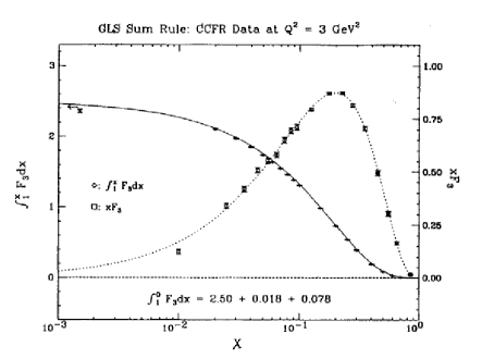
Figure 2: Experimental results for Gross-Llewellyn Smith sum rule, Eq. 10, from the CCFR group, Ref. CCFR . Squares: $x\overline{F}_{3}(x)$, sum of neutrinos plus antineutrinos, at $Q^{2}=3$ GeV². Dashed curve: analytic fit to $x\overline{F}_{3}$. Diamonds: approximation to the integral $S_{{\scriptscriptstyle GLS}}(x)$ of Eq. 11. Solid line: fit to the integral $S_{{\scriptscriptstyle GLS}}(x)$.

Fig. 2 shows the CCFR measurements on iron and the experimental values of $x\overline{F}_{3}^{WA}(x)$ (the sum of the nuclear $xF_{3}$ structure function for neutrinos plus that for antineutrinos) vs. $x$. The CCFR group measured cross sections at several values of $x$ and $Q^{2}$. The squares give the value of $x\overline{F}_{3}(x)$ interpolated to an average momentum transfer $Q^{2}=3$ GeV² (this is the mean $Q^{2}$ for the lowest $x$-bin in the CCFR experiment, since the lowest $x$ values contribute the greatest amount to the GLS sum rule). The dashed curve is the best fit to $x\overline{F}_{3}(x)$ of the form $Ax^{b}(1-x)^{c}$. This form was used to extrapolate the first moment to $x=0$. The CCFR reported value for the sum rule CCFR at this $Q^{2}$ value is $S_{GLS}=2.50\pm 0.018\ (stat)\pm 0.078\ (syst)$. The GLS sum rule is therefore known to about 3%.

The solid curve in Fig. 2 is $S_{{\scriptscriptstyle GLS}}(x)$. In the following sections we will consider additional QCD contributions. We will estimate each correction term as a function of $x$. The lowest $x$ value contributing to the Gross-Llewellyn Smith sum rule as measured by the CCFR group is $x_{min}=0.015$. We will calculate each contribution to the GLS sum rule as a function of $x$, and estimate the contribution $\delta S_{{\scriptscriptstyle GLS}}(x)|_{x=x_{min}}$.

Figure 3: Gross-Llewellyn Smith sum rule, and errors, for a series of experiments, in chronological order from top to bottom.

Fig. 3 shows the evolution over time of the GLS sum rule value. The measurements shown are from the CDHS CDHS2 , CHARM CHARM , CCFRR Macfar , and WA25 WA25 collaborations. There are also two points from the CCFR measurements, the first using the Narrow Band Beam (NBB) neutrino data NBB ; Mishra and the second using the QTB data CCFR from the Fermilab Tevatron.

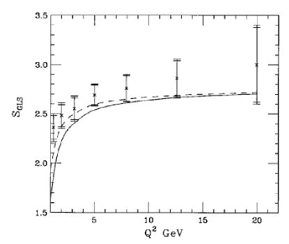
Figure 4: Results for the Gross-Llewellyn Smith sum rule, $S_{{\scriptscriptstyle GLS}}$ for various values of $Q^{2}$; from Ref. Hin96 . The inner error bars are statistical and the outer errors combine statistical and systematic errors. The data are from the CCFR experiment CCFR , and the solid and dashed curves are theoreteical QCD predictions from Hinchliffe and Kwiatkowski Hin96 ; the solid curve includes higher-twist effects while the dashed curve neglects them.

The points with error bars in Fig. 4 represent the experimental results from the CCFR group for the Gross-Llewellyn Smith sum rule as a function of $Q^{2}$. The curves are theoretical QCD predictions by Hinchliffe and Kwiatkowski Hin96 , using higher-order QCD corrections from Larin and Vermaseren larin , and higher-twist corrections of Braun and Kolesnichenko braun . The dashed curves are calculations without higher-twist effects, and the solid curves include higher-twist. The theoretical calculations appear to lie systematically below the experimental results by one to two standard deviations.

In the remainder of this paper we will review the steps that are taken to extract the $F_{3}$ structure functions from the experimental cross sections. We will then review the corrections to Eq. (9). In particular, we will focus on the contributions to the Gross-Llewellyn Smith sum rule from strange quarks and from charge symmetry violating contributions to parton distribution functions. Although these constitute fairly small corrections, nevertheless they may play an important role in determining the extent of the agreement, or disagreement, between theory and experiment for the GLS sum rule.

III Extracting Structure Functions from Neutrino and Antineutrino Cross Sections

The most precise neutrino and antineutrino DIS cross sections are those of the CCFR and NuTeV groups, both taken on iron targets. From Eq. (1) by taking sums and differences of differential cross sections for charged-current DIS from neutrino and antineutrino beams, we can isolate different combinations of structure functions. The CCFR and NuTeV experiments bin the data in $x$ and $Q^{2}$. Defining the quantity $c=\pi/{{G_{{\scriptscriptstyle F}}}^{2}}ME_{\nu}$, it is straightforward to show that

$$c\left[\frac{d^{2}\sigma^{\nu A}_{{\scriptscriptstyle CC}}}{dx\,dQ^{2}}+\frac{d^{2}\sigma^{{\overline{\nu}}A}_{{\scriptscriptstyle CC}}}{dx\,dQ^{2}}\right]=2f(y,Q^{2})\overline{F}_{2}^{WA}(x)$$ (13)

$$+ g(y,Q^{2})\Delta xF_{3}^{WA}(x)\ ;$$

$$c\left[\frac{d^{2}\sigma^{\nu A}_{{\scriptscriptstyle CC}}}{dx\,dQ^{2}}-\frac{d^{2}\sigma^{{\overline{\nu}}A}_{{\scriptscriptstyle CC}}}{dx\,Q^{2}}\right]=f(y,Q^{2})\Delta F_{2}^{WA}(x)$$

$$+ 2g(y,Q^{2})x\overline{F}_{3}^{WA}(x)\ .$$

In Eq. (13) the coefficients $f(y,Q^{2})$ and $g(y,Q^{2})$ are defined as

$$f(y,Q^{2})=\frac{yf_{1}(y)}{Q^{2}}=(1-y+\frac{y^{2}}{2(1+R_{L}^{\nu})})\frac{y}{Q^{2}};$$ (14)

$$g(y,Q^{2})=\frac{yf_{2}(y)}{Q^{2}}=(y-\frac{y^{2}}{2})\frac{y}{Q^{2}}.$$

The cross sections entering Eq. (13) have been normalized to give the correct total cross sections for neutrinos and antineutrinos. The procedure for this is described in the review by Conrad et al. Con98 . For the time being, we will consider the extraction of the structure function $xF_{3}^{WA}$ for an isoscalar target.

Previous analyses have neglected the term $\Delta F_{2}^{WA}(x)$ in Eq. (13). From Eq. (LABEL:eq:FApdf) we see that all contributions to this term should be small. We will neglect the $c^{-}$ term in Eq. (9) because, even though a mechanism has been identified which could produce such an asymmetry Melnitchouk:1997ig , the charm contribution is certainly suppressed substantially with respect to that associated with strange quarks and the charmed contribution is also kinematically suppressed for the experimental conditions – c.f. Eq. (37) in Sect. IV.4. Thus for an isoscalar target at sufficiently high $Q^{2}$ we expect

$$\Delta F_{2}^{WA}(x) \to 2xs^{-}(x)+x(-\delta u^{-}(x)+\delta d^{-}(x));$$

$$\Delta xF_{3}^{WA}(x) \to 2x(s^{+}(x)+c^{+}(x))$$

$$+ x(-\delta u^{+}(x)+\delta d^{+}(x)).$$

From Eq. (LABEL:eq:FApdfN) we see that for an isoscalar target the term $\Delta F_{2}^{WA}(x)$ will be non-zero only if one has a strange quark momentum asymmetry $s^{-}(x)\neq 0$, and/or non-zero valence quark CSV contributions. In Sect. IV.4 we will discuss additional contributions to $\Delta F_{2}^{WA}(x)$ for a non-isoscalar target.

If one neglects the term $\Delta F_{2}^{WA}(x)$ in Eq. (13) (as was the case in the analysis of the CCFR data), then the structure function $x\overline{F}_{3}^{WA}(x)$ will just be proportional to the difference between the neutrino and antineutrino charged-current DIS cross sections. For a given $x$ bin, the structure function $xF_{3}$ is then given by averaging the structure function differences over the $Q^{2}$ bin appropriate to the given $x$ bin. Thus we obtain

$$x\overline{F}_{3}^{WA}(x) = \frac{c}{2A(x)}\int_{\langle Q^{2}\rangle}\left[\frac{d^{2}\sigma^{\nu A}_{{\scriptscriptstyle CC}}}{dx\,dQ^{2}}-\frac{d^{2}\sigma^{{\overline{\nu}}A}_{{\scriptscriptstyle CC}}}{dx\,Q^{2}}\right]\,dQ^{2},$$

$$A(x) = \int_{\langle Q^{2}\rangle}g(y,Q^{2})dQ^{2}\ .$$ (16)

In Eq. (16), $\langle Q^{2}\rangle$ denotes the average over the $Q^{2}$ bin appropriate to a given $x$ bin. In Eq. (16), we have neglected the slow variation of $\overline{F}_{3}^{WA}$ with $Q^{2}$.

However, if the quantity $\Delta F_{2}^{WA}(x)$ is non-zero, then Eq. (16) will not give the structure function $x\overline{F}_{3}^{WA}(x)$, but rather a linear combination of $xF_{3}$ and $\Delta F_{2}$. Comparing this with Eq. (13), we note that the $y$ dependence of the coefficients $f$ and $g$ of the two terms is quite different, as shown in Eq. (14). In particular, the coefficient of $x\overline{F}_{3}^{WA}$ vanishes at $y=0$, while the coefficient of $\Delta F_{2}^{WA}$ is finite. Inserting Eq. (13) into Eq. (16) and averaging over the $Q^{2}$ range for each $x$ bin gives

$$\frac{c}{2A(x)}\int_{\langle Q^{2}\rangle}\left[\frac{d^{2}\sigma^{\nu A}_{{\scriptscriptstyle CC}}}{dx\,dQ^{2}}-\frac{d^{2}\sigma^{{\overline{\nu}}A}_{{\scriptscriptstyle CC}}}{dx\,Q^{2}}\right]\,dQ^{2}$$ (17)

$$= x\overline{F}_{3}^{WA}(x)+B(x)\Delta F_{2}^{WA}(x),$$

$$B(x)=\frac{\int_{\langle Q^{2}\rangle}f(y,Q^{2})dQ^{2}}{2A(x)}\ .$$

The quantity $B(x)$ in Eq. (17) is the relative weighting between the $\Delta F_{2}$ and $xF_{3}$ terms. $B(x)$ will depend upon the $x$ bin and the $Q^{2}$ values that are averaged over for each $x$ bin. In Fig. 5 we plot the ratio $f(y,Q^{2})/g(y,Q^{2})$ in Eq. (13) vs. $y$ (this quantity is identical to the ratio $f_{1}(y)/f_{2}(y)$ from Eq. (1)). This ratio is always greater than one, and becomes quite large at small $y$ values. The quantity $B(x)$ is normalized to equal one if one integrates over all $y$; however $B(x)$ could be greater than one particularly if the average over $Q^{2}$ is weighted towards small $y$ values.

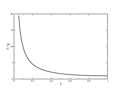
Figure 5: The quantity $f(y,Q^{2})/g(y,Q^{2})$ from Eq. (13) plotted versus $y$, under the assumption that $R_{L}^{\nu}=0$; it is identical to $f_{1}(y)/f_{2}(y)$ defined in Eq. (1).

Eq. (17) shows that for an isoscalar target, the common process of taking the difference of neutrino and antineutrino charged-current cross sections, and averaging over the $Q^{2}$ bin for a given $x$ bin produces a linear combination of $x\overline{F}_{3}^{WA}$ and $\Delta F_{2}^{WA}$ with a relative weighting $B(x)$. From Eq. (LABEL:eq:FApdf) we see that the partonic content of the quantity identified as $x\overline{F}_{3}$ will be

$${}^{\prime\prime}x\overline{F}_{3}^{WA}(x)^{\prime\prime}=x\overline{F}_{3}^{WA}(x)+B(x)\Delta F_{2}^{WA}(x)$$

$$= x\bigl{[}u^{-}(x)+d^{-}(x)+s^{-}(x)(1+2B(x))$$

$$+ \delta d^{-}(x)(B(x)-\frac{1}{2})-\delta u^{-}(x)(B(x)+\frac{1}{2})\bigr{]}.$$

We put quotes around the quantity $x\overline{F}_{3}^{WA}$, since it represents the linear combination of $x\overline{F}_{3}^{WA}$ and $\Delta F_{2}^{WA}$ obtained for that $x$ bin. As we have mentioned, the $y$ dependence of the coefficients $f(y,Q^{2})$ and $g(y,Q^{2})$ in Eq. (13) is quite different, particularly in the forward direction. When the longitudinal to transverse ratio $R_{L}^{\nu}=0$, the ratio $f(y,Q^{2})/g(y,Q^{2})$ is given in Fig. 5. If we assume that for each $x$ bin, the data is averaged over all $y$, then one obtains $B(x)=1$, and Eq. (LABEL:eq:F3extract) becomes

$${}^{\prime\prime}x\overline{F}_{3}^{WA}(x)^{\prime\prime}|_{B(x)=1}=x\biggl{[}u^{-}(x)+d^{-}(x)$$

$$+ 3s^{-}(x)+\frac{\delta d^{-}(x)-3\delta u^{-}(x)}{2}\biggr{]}.$$

These additional terms should be included in the analysis of the experimental data. In the absence of such an analysis we will provide estimates of the sign and magnitude of these corrections and their effect on the Gross-Llewellyn Smith sum rule.

IV Additional Corrections to the GLS Sum Rule

In addition to contributions from the light valence quarks, higher order QCD terms and higher twist contributions, Eq. (10) contains additional QCD corrections. These corrections are included in the experimental determination of the GLS sum rule, but these additional terms have not been included in theoretical calculations. There are two types of corrections. The first involves additional contributions to the desired term $x\overline{F}_{3}^{WA}$ in Eq. (LABEL:eq:FApdf). The second contribution appears by virtue of the term $\Delta F_{2}^{WA}$, which has not been separated from the desired term. In both cases we include contributions from strange quarks and partonic CSV corrections. Although the first moment of each of these contributions vanishes when integrated over all $x$, there is a residual contribution still present at $x_{min}=0.015$, the lowest data point in the CCFR experiment. In order to reconcile theoretical and experimental determination of the GLS sum rule, we choose to subtract these additional contributions from the experimental data when comparing with theory. We define the corrections to the GLS sum rule as

$$\delta S_{{\scriptscriptstyle GLS}}={\rm lim}_{x\rightarrow 0}\ \delta S_{{\scriptscriptstyle GLS}}(x).$$ (20)

For an isoscalar target these corrections have the form

$$\delta S_{{\scriptscriptstyle GLS}}(x) = f({\alpha_{{\scriptscriptstyle S}}})\left[\delta S_{{\scriptscriptstyle GLS}}^{s}(x)+\delta S_{{\scriptscriptstyle GLS}}^{{\scriptscriptstyle CSV}}(x)\right]\ ,$$

$$\delta S_{{\scriptscriptstyle GLS}}^{s}(x) = \int_{x}^{1}s^{-}(y)(2B(y)+1)\,dy\ ,$$

$$\delta S_{{\scriptscriptstyle GLS}}^{{\scriptscriptstyle CSV}}(x) = \int_{x}^{1}\biggl{[}(B(y)-\frac{1}{2})\delta d^{-}(y)$$ (21)

$$- (B(y)+\frac{1}{2})\delta u^{-}(y)\biggr{]}\,dy$$

The term $f({\alpha_{{\scriptscriptstyle S}}})$ in Eq. (21) is the QCD correction that has been calculated by Larin and Vermaseren larin ; it is the term in square brackets in Eq. (10).

Eq. (21) contains two terms. The first is the contribution from the strange quark asymmetry. The second is the contribution from charge symmetry violating valence PDFs. An additional effect will result from the nuclear modification of the parton distributions. Implicitly, all of the parton distribution functions in Eq. (21) denote parton distributions in iron. In Sect. IV.4 we will discuss nuclear modifications of the PDFs. Note that the terms containing the quantity $B(y)$ result from the contamination of the $x\overline{F}_{3}$ structure function from the $\Delta F_{2}$ term.

If the quantity $B(y)$ in Eq. (21) was a constant, then both the strange and CSV terms would give zero in the limit $x\rightarrow 0$. This is because valence quark normalization requires that the valence strange quark and valence CSV PDFs have zero first moment. However, we have no reason to believe that $B(y)$ will be constant. Note also that the $C$-odd strange quark and valence CSV effects contribute to $\delta S_{{\scriptscriptstyle GLS}}(x)$ at any finite value of $x$. So even if the quantity $B(y)$ were a constant, the CSV and strange quark effects would be finite for any non-zero value of $x$, vanishing only at $x=0$.

From our current understanding of the parton distributions, for sufficiently large $x$ we expect every term in the quantity $\Delta F_{2}^{WA}(x)$ in Eq. (LABEL:eq:FApdfN) to have the same sign. As we shall see, all of the latest analyses of strange quark distributions Mason:2007zz ; Lai:2007dq ; Martin:2009iq ; Ball:2009mk ; Alekhin:2008mb find that the quantity $s^{-}(x)$ is positive for sufficiently large $x$. Analyses of parton valence charge symmetry violating effects for parton distributions Londergan:2009kj obtain a quantity $\delta d^{-}(x)-\delta u^{-}(x)>0$ for $x\geq 0.1$. Consequently, both of the terms in $\delta S_{{\scriptscriptstyle GLS}}$ in Eq. (21) will contribute with the same sign. In the following sections we will estimate the magnitude of each of these contributions.

IV.1 Corrections to the GLS Sum Rule at $Q^{2}=8$ GeV²

For convenience we calculate the corrections associated with a strange quark asymmetry and parton charge symmetry violation at a single value of $Q^{2}$, and we choose $Q^{2}=8$ GeV². From Fig. 4 we see that this is a value of $Q^{2}$ for which the experimental GLS sum rule has been measured. It is also a relatively convenient value of $Q^{2}$ for which to estimate corrections from both strange quarks and parton CSV. At $Q^{2}=8$ GeV², the experimental value of the Gross-Llewellyn Smith sum rule is $S_{{\scriptscriptstyle GLS}}^{exp}=2.76\pm 0.14$, and the theoretical value of Hinchliffe and Kwiatkowski Hin96 including higher-twist corrections is $S_{{\scriptscriptstyle GLS}}^{th}=2.62$. So the theoretical value is just over one standard deviation below the experimental result.

In the next sections we will provide estimates for the strange quark and partonic CSV contributions to the GLS sum rule. After evaluating them we will determine the correction that they make to the experimental value and error for the Gross-Llewellyn Smith sum rule for this value of $Q^{2}$.

The QCD correction that appears in Eq. (21) was evaluated by Larin and Vermaseren larin ; it has the form

$$f({\alpha_{{\scriptscriptstyle S}}})=1-\frac{{\alpha_{{\scriptscriptstyle S}}}}{\pi}-\left(\frac{{\alpha_{{\scriptscriptstyle S}}}}{\pi}\right)^{2}r_{1}-\left(\frac{{\alpha_{{\scriptscriptstyle S}}}}{\pi}\right)^{3}r_{2}\ ,$$ (22)

where for $n_{f}=3$ active flavors one has $r_{1}=3.5833$ and $r_{2}=18.9757$ larin . For the strong coupling ${\alpha_{{\scriptscriptstyle S}}}$ we use the value chosen by Hinchliffe and Kwiatkowski Hin96 in their theoretical calculations. In the ${\overline{MS}}$ factorization scheme they chose the scale parameter $\Lambda^{(5)}_{{\overline{MS}}}=233$ MeV; here the superscript denotes $n_{f}$. This corresponds to $\Lambda^{(3)}_{{\overline{MS}}}=366$ MeV and a strong coupling ${\alpha_{{\scriptscriptstyle S}}}(Q^{2}=3~{}GeV^{2})=0.336$. Using this value we then obtain $f({\alpha_{{\scriptscriptstyle S}}})(Q^{2}=8~{}GeV^{2})=0.885$.

IV.2 Contributions from Strange Quarks

The strange quark parton distributions are best obtained from an analysis of opposite-sign dimuon production in reactions induced by neutrinos and antineutrinos. In such reactions, dimuon production from a $\nu$ (${\overline{\nu}}$) beam is sensitive to the $s$ ($\bar{s}$) distribution, so that in principle a comparison of these cross sections could enable one to determine differences between the $s$ and $\bar{s}$ PDFs. There are recent measurements of these reactions by the CCFR and NuTeV Baz95 ; Gon01 ; Mason:2007zz collaborations. In the CCFR experiment the $\nu$ and ${\overline{\nu}}$ beams were not separated and the type of reaction was inferred from the charge of the faster muon, while the NuTeV experiment used separated $\nu$ and ${\overline{\nu}}$ beams.The correction to the GLS sum rule is obtained from

$$\delta S_{{\scriptscriptstyle GLS}}^{s}(x)=\int_{x}^{1}s^{-}(y)(2B(y)+1)\,dy$$ (23)

Now, the first moment of $s^{-}$ is zero, from valence quark normalization (there are no net “strange valence” quarks in the nucleon). However, recent phenomenological analyses of strange quark distributions all obtain qualitatively similar results. All of them find the most probable value is a positive strange quark momentum asymmetry, $\langle xs^{-}(x)\rangle>0$. Also, the best fit to the quantity $s^{-}(x)$ changes sign at an extremely small value of $x$ and is large and positive down to rather small $x$ values.

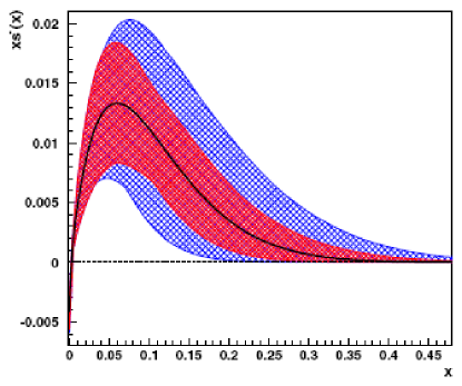
Figure 6: [color online] The quantity $xs^{-}(x)=x[s(x)-\bar{s}(x)]$, vs. $x$, as extracted by the NuTeV Collaboration, Ref. Mason:2007zz . Values are obtained for $Q^{2}=16$ GeV². The outer error band is the combined error, while the inner band is without the uncertainty in the semileptonic branching ratio $B_{c}$.

For example, the analysis by Mason et al. Mason:2007zz obtains a best value for the the integral of $xs^{-}(x)$

$$S^{-} = 0.00196\pm 0.00046(stat)\pm 0.00045(syst)$$ (24)

$${}^{+0.00148}_{-0.00107}(external).$$

The quantity $Q$ refers to the second moment of a parton distribution $q(x)$, i.e.

$$Q\equiv\int_{0}^{1}x\,q(x)\,dx$$ (25)

The Mason result is obtained for a value $Q^{2}=16$ GeV². In Eq. (24), the term “external” refers to the contribution arising from uncertainties on external measurements.

Fig. 6 plots the quantity $xs^{-}(x)$ vs. $x$ from the latest NuTeV analysis. The strange quark momentum asymmetry, $S^{-}$, is quite sensitive to two quantities. The first is the semileptonic branching ratio $B_{c}$; the outer band in Fig. 6 shows the result for $S^{-}$ with the $B_{c}$ uncertainty, and the inner band is the result without the $B_{c}$ uncertainty. The second is the point at which the distribution $xs^{-}(x)$ crosses zero (it must cross zero at least once to give zero first moment for $s^{-}(x)$). The current best fit crosses zero at a very small value $x\sim 0.004$. This means that the quantity $s^{-}(x)$ would have a large negative spike at extremely low $x$ (in fact, an $x$ value smaller than the lowest $x$ point measured in the experiment).

	$S^{-}=\langle xs^{-}\rangle$	$x_{0}$	$Q^{2}$ (GeV2)
Mason et al. Mason:2007zz	$0.00196\pm 0.00143$	$0.004$	$16$
CTEQ Lai:2007dq	$0.0018_{-0.0004}^{+0.0016}$	$0.01-0.02$	$1.69$
NNPDF Ball:2009mk	$0.0005\pm 0.0086$	$0.13$	$20$
MSTW Martin:2009iq	$0.0016_{-0.0009}^{+0.0011}$	$0.016$	$1.0$
Alekhin et al. Alekhin:2008mb	$0.0013\pm 0.0009\pm 0.0002$	$\leq 0.02$	$8$

Table 1: A summary of recent phenomenological estimates of the strangeness asymmetry ($S^{-}$ ), the crossover point $x_{0}$ and the $Q^{2}$ value at which the asymmetry is obtained.

There are several other recent phenomenological estimates of the strange quark asymmetry. All are very sensitive to the CCFR and NuTeV dimuon production data. The CTEQ group Lai:2007dq obtains $S^{-}=0.0018^{+0.0016}_{-0.0004}$ at their starting scale $Q_{0}^{2}=1.69$ GeV². Their best fits to $xs^{-}(x)$ found crossovers in the vicinity $x_{0}\sim 0.01-0.02$. The NNPDF Collaboration Ball:2009mk used only the NuTeV data and not the CCFR results. They report a value $S^{-}=0.0005\pm 0.0086$ at $Q^{2}=20$ GeV²; the exceptionally large error in the NNPDF value (a factor of 5 to 6 larger than the errors from the other analyses) results in part from their use of a neural network procedure, which does not build in widely accepted constraints on the shape of sea quark distributions.

Two other groups supplemented the NuTeV and CCFR dimuon data with charm production data from CHORUS KayisTopaksu:2005je ; Onengut:2005kv , which helps to constrain the semileptonic branching ratio. The MSTW group Martin:2009iq obtains $S^{-}=0.0016^{+0.0011}_{-0.0009}$ at $Q^{2}=10$ GeV²; their next to leading order (NLO) fit had a crossover $x_{0}=0.016$ at the starting scale $Q_{0}^{2}=1$ GeV². Alekhin, Kulagin and Petti Alekhin:2008mb obtained $S^{-}=0.0013\pm 0.0009\pm 0.0002$ at $Q^{2}=8$ GeV², and their best fit to $xs^{-}(x)$ had a crossover $x_{0}\leq 0.02$. For these various phenomenological fits we summarize the values of $S^{-}$, the crossover point $x_{0}$ and the value of $Q^{2}$ at which the asymmetry is calculated in Table I.

From Eq. (23) the contribution to the GLS sum rule from strange quarks, for a given value of $x$, will be given by the integral of $s^{-}(y)$ weighted by the quantity $2B(y)+1$. If we approximate $B(y)$ as a constant we just need the integral of $s^{-}(y)$ from $x$ to $1$. We choose the smallest value $x_{min}=0.015$ measured by CCFR. To estimate the integral we made an analytic fit to the strange asymmetry measured by Mason et al., in the region $x\geq 0.004$ Mason:2007zz . Our fit had the form $s^{-}(x)=ax^{b}e^{-cx}(x-0.004)$. With this fit we obtain the result

$$\int_{x=0.015}^{1}s^{-}(y)dy\approx 0.026.$$ (26)

Within their error bars, all of the phenomenological fits now obtain a positive value for the strange quark momentum asymmetry. Because of their unusually large error on the strange quark asymmetry and its unphysically large value in the valence region, we do not use the NNPDF result. All of the other fits to the strange quark PDFs produce a quantity $xs^{-}(x)$ which changes sign at an extremely small value of $x$. Thus all of these strange quark PDFs will give a reasonably large contribution to the GLS sum rule at a value of $x$ corresponding to the lowest $x$ value measured in the CCFR experiment. We assign an error of 75% which is roughly the average of the four determinations (excluding NNPDF) summarized in Table I. Thus we choose

$$\int_{x=0.015}^{1}s^{-}(x)dx=0.031\pm 0.023.$$ (27)

In Eq. (27) we have increased the integral of this distribution by 20%; this represents the approximate increase in this moment in evolving from $Q^{2}=16$ GeV² to the value $Q^{2}=8$ GeV² appropriate for our evaluation of the GLS sum rule. This increase is comparable to results obtained by the NNPDF group Ball:2009mk , who performed DGLAP evolution on the second moment of strange quark distributions to extrapolate in $Q^{2}$.

From Eq. (23), the strange quark asymmetry contribution to the GLS sum rule will depend on estimates of $B(x)$. We make two simple guesses for this quantity. First, we take $B(x)=1$; this is the result if the integral of Eq. (17) was taken over all $y$. Next, we estimate $B(x)=2$; this represents an upper limit (and possibly an overestimate) of this quantity. Under these approximations we obtain strange corrections to the GLS sum rule

$$\delta S_{{\scriptscriptstyle GLS}}^{s} = 0.093\pm 0.063\ ,~{}{\rm for}~{}B(x)=1\ ;$$

$$\delta S_{{\scriptscriptstyle GLS}}^{s} = 0.156\pm 0.115\ ,~{}{\rm for}~{}B(x)=2\ .$$ (28)

The large result for the strange quark contribution results from the fact that the strange quark momentum asymmetry changes sign at an extremely small value of $x$. Although we have used the result of Mason et al., this property is shared by all phenomenological strange quark analyses in Table I except for NNPDF.

The contribution from the strange momentum asymmetry to the GLS sum rule is strongly dependent on the crossover point $x_{0}$ at which $s^{-}(x)$ crosses zero. If the crossover point for $s^{-}(x)$ occurred at a value $x_{0}\geq 0.1$ then strange quarks would make an extremely small contribution to the GLS sum rule. It is difficult to imagine a physical mechanism that would cause $s^{-}(x)$ to change sign at such small crossover points $x_{0}$ as have been found in these phenomenological analyses Mason:2007zz ; Lai:2007dq ; Martin:2009iq ; Alekhin:2008mb . Indeed, model calculations almost invariably yield a zero at $x\sim 0.1$ or higher Signal:1987gz ; Melnitchouk:1999mv ; Carvalho:2005nk ; Wei:2007nb . The NuTeV group found that with a moderate increase in $\chi^{2}$ one could obtain considerably larger values of $x_{0}$ and corresponding large decreases in the second moment $S^{-}$ Mason:2007zz .

IV.3 Contributions from Charge Symmetry Violating PDFs

We also can estimate the contribution from parton CSV. For an isoscalar target this is given by

$$\delta S_{{\scriptscriptstyle GLS}}^{{\scriptscriptstyle CSV}}(x) = \int_{x}^{1}\bigl{[}(B(y)-\frac{1}{2})\delta d^{-}(y)$$ (29)

$$- (B(y)+\frac{1}{2})\delta u^{-}(y)\bigr{]}\,dy$$

For this we need the valence CSV parton distribution functions Londergan:2009kj . We adopt the functional form used by the MRST group MRST03 ,

$$\delta u^{-}(x)=-\delta d^{-}(x)=\kappa x^{-0.5}(1-x)^{4}(x-.0909)$$ (30)

The best fit value of MRST was $\kappa=-0.2$. This produced contributions very much like the quark model valence CSV calculations of Rodionov et al. Rod94 evaluated at $Q^{2}=10$ GeV². Here we choose $\kappa=-0.3$, which approximates quite well the quark model valence CSV from Rodionov, plus the valence CSV arising from “QED splitting” MRST05 ; Glu05 . If we assume that $\delta d^{-}(x)=-\delta u^{-}(x)$, then from Eq. (10) the term $S_{{\scriptscriptstyle GLS}}^{{\scriptscriptstyle CSV}}(x)$ in Eq. (29) has the form

$$\delta S_{{\scriptscriptstyle GLS}}^{{\scriptscriptstyle CSV}}(x)=-2\,\int_{x}^{1}B(y)\delta u^{-}(y)\,dy\ .$$ (31)

We insert the analytic form of Eq. (30) into Eq. (31) and evaluate at $x_{min}=0.015$, the minimum $x$ value for the CCFR measurements. As for the strange quark contribution we evaluate this using two different values for the weighting function, $B(y)=1$ and $B(y)=2$. We assign a 100% error to the CSV contribution. Thus we obtain

$$\delta S_{{\scriptscriptstyle GLS}}^{{\scriptscriptstyle CSV}} = 0.013\pm 0.013\ ,{\rm B(y)~{}=1}$$ (32)

$$= 0.026\pm 0.026\ ,{\rm B(y)~{}=2}$$

The partonic charge symmetry violating contributions correspond to a value $Q^{2}\sim 10$ GeV². This is sufficiently close to the value $Q^{2}=8$ GeV² that we do not modify this further.

IV.4 Non-Isoscalar and Nuclear Corrections

Until now our equations have assumed an isoscalar target. We must include corrections to account for the excess neutrons in iron. From Eq. (LABEL:eq:FApdf) there are a number of small corrections in the case that $N\not=Z$. For our purposes the most important will be an additional contribution to the quantity $\Delta F_{2}^{WA}(x)$ of the form

$$\delta(\Delta F_{2}^{WA}(x))={\nu_{f}}x[u^{-}(x)-d^{-}(x)]\ .$$ (33)

When multiplied by the quantity $B(x)$, divided by $x$ and integrated over all $x$, this leads to the contribution

$$\delta S_{{\scriptscriptstyle GLS}}^{{\nu_{f}}}(x)={\nu_{f}}\,\int_{x}^{1}B(y)[u^{-}(y)-d^{-}(y)]\,dy\ .$$ (34)

For convenience we take the lower limit of this integral to be $x=0$; in the limit where $B(x)$ is approximated as a constant, $B(x)\sim B$, the remaining integral is just one, so in this approximation we obtain

$$\delta S_{{\scriptscriptstyle GLS}}^{{\nu_{f}}} \approx {\nu_{f}}B\ ,$$ (35)

$$= 0.058,\hskip 11.38092pt{\rm for}~{}B(x)=1;$$

$$= 0.115,\hskip 11.38092pt{\rm for}~{}B(x)=2.$$

Note that all of the contributions to the GLS sum rule (strange quark asymmetry, quark model valence CSV and QED splitting CSV, and non-isoscalar effects) are of the same sign. Thus, their contributions will add coherently in modifying the GLS sum rule.

The contributions listed here for strange quarks, CSV parton distributions and $N\not=Z$ effects were included in the experimental results but not in the theoretical calculations of Hinchliffe and Kwiatkowski Hin96 . Consequently we choose to subtract these contributions from the experimental results, in order to compare with theory. At $Q^{2}=8$ GeV² the quoted experimental result for the Gross-Llewellyn Smith sum rule was $2.76\pm 0.14$. We take the strange quark contribution from Eq. (28), the CSV contribution from Eq. (32), and the $N\not=Z$ contribution from Eq. (35). These effects are multiplied by the QCD correction factor $f(\alpha_{s})$ from Eq. (22). We assume that the errors can be combined in quadrature. This leads to the net result

$$S_{{\scriptscriptstyle GLS}}^{expt}|_{Q^{2}=8~{}GeV^{2}} \to 2.62\pm 0.15,~{}{\rm B(y)~{}=1}$$

$$\to 2.50\pm 0.17,~{}{\rm B(y)~{}=2}\ .$$

We can compare this with the theoretical value $S_{{\scriptscriptstyle GLS}}^{th}=2.62$. We see that these additional terms improve the agreement between theory and experiment. In the approximation $B(y)=1$ there is now excellent agreement between theory and experiment; when $B(y)=2$ the experimental point is now below the data but still within one standard deviation. Since the errors are added in quadrature, the net result is a small increase in the overall error.

For the purpose of completeness we will review the corrections that were applied to the experimental data by the CCFR group. Before solving for the structure functions from the neutrino and antineutrino cross sections (see Eq. (13) and following equations), the CCFR collaboration made a series of corrections to the cross sections. First, as we have mentioned previously, the neutrino and antineutrino cross sections were normalized to the total fluxes. Next, the cross sections were multiplied by four nuclear correction factors,

$$\sigma^{corr}=\sigma^{iso}\times\sigma^{rad}\times\sigma^{c}\times\sigma^{W}\ .$$ (37)

In Eq.(37), the term $\sigma^{rad}$ includes the radiative corrections to the cross sections, calculated from the prescription of Bardin and Dokochueva Bar86 . The term $\sigma^{c}$ represents a correction for the finite charm quark mass since the data, particularly at low $Q^{2}$, is taken in a region close to charm quark threshold. The term $\sigma^{W}$ is a correction for the finite $W$ mass. The remaining correction, $\sigma^{iso}$, was an attempt to account for the neutron asymmetry in iron. We will review this correction in some detail.

On average for the CCFR target, the neutron excess is given by ${\nu_{f}}=(N-Z)/A=0.0567$ Sel97a . The CCFR group made an “isoscalar correction” to the neutrino and antineutrino cross sections. They calculated the quark and antiquark neutrino momentum densities on iron, via the $F_{2}$ structure functions per nucleon for $\nu$ and ${\overline{\nu}}$ on a non-isoscalar target,

$$xq^{\nu A}(x)=2x\bigl{[}{\frac{Z}{A}}(d^{p}(x)+s^{p}(x))$$ (38)

$$+ {\frac{N}{A}}(d^{n}(x)+s^{n}(x))\bigr{]}$$

$$= x(1-{\nu_{f}})d(x)+x(1+{\nu_{f}})u(x)+2xs(x);$$

$$x{\overline{q}}^{\nu A}(x)=x(1-{\nu_{f}}){\overline{u}}(x)+x(1+{\nu_{f}}){\overline{d}}(x);$$

$$xq^{{\overline{\nu}}A}(x)=x(1-{\nu_{f}})u(x)+x(1+{\nu_{f}})d(x);$$

$$x{\overline{q}}^{{\overline{\nu}}A}(x)=x(1-{\nu_{f}}){\overline{d}}(x)+x(1+{\nu_{f}}){\overline{u}}(x)$$

$$+2x{\overline{s}}(x)\ .$$

The cross sections were then re-normalized by the “isoscalar correction factor,”

$$corr^{iso}\equiv\frac{\sigma({\rm isoscalar~{}target})}{\sigma({\rm Fe~{}target})}=\frac{\sigma({\nu_{f}}=0)}{\sigma({\nu_{f}}=0.0567)}$$ (39)

The isoscalar correction is different for neutrinos and for antineutrinos. Note that this process is circular – the isoscalar correction applied to the cross sections requires knowledge of the parton distributions, which are themselves extracted from the cross sections. Thus the process was applied iteratively. An isoscalar correction was applied to the cross sections from Eq. (39) using the parton distributions from Eq. (38). The structure functions were then determined by inserting the renormalized cross sections into Eq. (13). From the structure functions one can extract new parton distributions, from which a new isoscalar correction factor could be determined. The process was then iterated until the difference in the extracted structure functions became sufficiently small.

The isoscalar correction factor applied by the CCFR collaboration should account for most of the neutron asymmetry corrections. However, after this correction has been applied it is then difficult to isolate the remaining contribution from the $\Delta F_{2}^{WA}$ term in Eq. (13). Certainly there is a term present in the coupled equations, which has not been accounted for by the CCFR group. It should be straightforward to include this term in any re-analysis of neutrino cross section data. One could add this as a perturbation and could obtain decent estimates of the strange quark and CSV contributions as outlined in Sect. III.

The sign and magnitude of the strange and CSV contributions should be similar to our estimate of these terms for an isoscalar target. There may also be small additional contributions from neutron asymmetry to $xF_{3}$, which have not been accounted for by the isoscalar correction made by CCFR. We have not made further corrections for any nuclear modification of the parton distributions in iron. Several groups have estimated the magnitude of nuclear effects on parton distribution functions Kum02 ; Hir04 ; Hir05 ; Kul06 ; Kul07 ; Kul07b ; Cloet:2009qs .

V Conclusions

The Gross-Llewellyn Smith sum rule is obtained from the first moment of the structure function $xF_{3}$ from neutrino charged-current deep inelastic scattering. In principle these structure functions can be obtained by comparing sums and differences of neutrino and antineutrino DIS cross sections on an isoscalar nucleus. Previous analyses of the GLS sum rule have neglected potential contributions from strange quark asymmetries and from partonic charge symmetry violation. At the time, such contributions were largely unknown and could be assumed to be negligibly small.

However, recently one has more quantitative results for strange quark asymmetries from several groups Mason:2007zz ; Martin:2009iq ; Lai:2007dq ; Ball:2009mk ; Alekhin:2008mb . All of these analyses rely on measurements of opposite-sign dimuon production in neutrino and antineutrino reactions on iron from the CCFR and NuTeV collaborations Baz95 ; Gon01 . All of these analyses obtained a positive value for $\langle xs^{-}(x)\rangle$; with the exception of tne NNPDF analysis Ball:2009mk (which used a neural network approach, was relatively insensitive to the $s$ quark distribution and obtained very large error bars), these analyses found a crossover point for the $s^{-}(x)$ PDFs that occurred at an extremely small value $x_{0}\approx 0.01$. We chose as an example the strange quark analysis by the NuTeV group, Mason et al. Mason:2007zz , but the correction to the GLS sum rule arising from the strange quark asymmetry should be quite similar if one used instead the CTEQ Lai:2007dq , MSTW Martin:2009iq or Alekhin Alekhin:2008mb analyses.

Furthermore, one now has reasonable estimates for contributions from valence quark CSV. First, there are now phenomenological analyses of parton distributions that include partonic CSV MRST03 . Second, there have been calculations of partonic CSV arising from the different electromagnetic coupling of photons to up and down quarks MRST05 ; Glu05 . Finally, there are quark model calculations of partonic CSV Londergan:2009kj . We used these to estimate the partonic CSV contribution to the Gross-Llewellyn Smith sum rule. Finally, we estimated the contribution to the GLS sum rule from the fact that iron is a non-isoscalar target.

The correct procedure would be to incorporate these effects into the initial analysis of the neutrino cross sections. In particular one should take into account the effect of the term $\Delta F_{2}^{WA}(x)$ in Eq. (LABEL:eq:FApdf). Since this term has not been included in previous analyses of neutrino cross sections we can only estimate its effect on the Gross-Llewellyn Smith sum rule. This has been carried out in this paper. To summarize our conclusions: first, the contributions from strange quarks, parton CSV and non-isoscalar effects all appear to have the same sign and hence to add coherently; second, we estimate that these effects should contribute an amount on the order of one to two standard deviations in the GLS sum rule; third, we find that inclusion of all of these contributions should bring the theoretical and experimental determinations of the GLS sum rule in agreement within $1\sigma$. In Sect. IV.4 we noted that the cross section corrections adopted by the CCFR group make it difficult to provide quantitative estimates of the effects of strange quarks and partonic charge symmetry violation to the Gross-Llewellyn Smith sum rule. Nevertheless, if these corrections were to be integrated into a re-analysis of the neutrino cross sections, one should be able to obtain an accurate quantitative assessment of the contributions from these quantities.