Wannier representation of $\mathbb{Z}_{2}$ topological insulators

Abstract

We consider the problem of constructing Wannier functions for $\mathbb{Z}_{2}$ topological insulators in two dimensions. It is well known that there is a topological obstruction to the construction of Wannier functions for Chern insulators, but it has been unclear whether this is also true for the $\mathbb{Z}_{2}$ case. We consider the Kane-Mele tight-binding model, which exhibits both normal ($\mathbb{Z}_{2}$-even) and topological ($\mathbb{Z}_{2}$-odd) phases as a function of the model parameters. In the $\mathbb{Z}_{2}$-even phase, the usual projection-based scheme can be used to build the Wannier representation. In the $\mathbb{Z}_{2}$-odd phase, we do find a topological obstruction, but only if one insists on choosing a gauge that respects the time-reversal symmetry, corresponding to Wannier functions that come in time-reversal pairs. If instead we are willing to violate this gauge condition, a Wannier representation becomes possible. We present an explicit construction of Wannier functions for the $\mathbb{Z}_{2}$-odd phase of the Kane-Mele model via a modified projection scheme followed by maximal localization, and confirm that these Wannier functions correctly represent the electric polarization and other electronic properties of the insulator.

I INTRODUCTION

In the past several years there has been a surge of interest in topological insulators. These are materials that are gapped in the bulk, just like ordinary insulators, but that cannot be adiabatically connected to ordinary insulators without closing the gap or breaking some specified symmetries. They also exhibit chiral metallic edge states that are topologically protected from disorder.Schnyder-PRB08 ; Schnyder-AIP09 ; Kitaev-AIP09 Topological insulators can be distinguished from normal ones based on the manner in which the Bloch eigenfunctions are topologically twisted in k-space.

Two types of topological insulators have received the most attention. First, Thouless et al.Thouless-PRL82 pointed out long ago that a two-dimensional (2D) insulator is characterized in general by a topological integer known as the “Chern number” or “TKNN index.” A prospective insulator having a non-zero value of this integer would be known as a “Chern” or “quantum anomalous Hall” insulator. The latter name arises because such a crystal would exhibit a quantum Hall effect (QHE) even in the absence of a macroscopic magnetic field, and would have chiral edge states just like the ordinary field-induced QHE. Haldane devised an explicit tight-binding model realizing such a case.Haldane-PRL88 Since the Hall conductance is odd under the time-reversal ($T$) operator, Chern insulators can only be realized in systems with broken $T$ symmetry, e.g., insulating ferromagnets. Despite the fact that these possibilities have been appreciated now for almost three decades, no known experimental realizations of a Chern insulator are yet known.

Second, a great deal of interest has surrounded the recent discovery of a different class of topological insulators known as $\mathbb{Z}_{2}$ insulators that realize the quantum spin Hall effect (QSH).Kane-PRL05-b Subsequent theoreticalBernevig-Science06 ; Zhang-NatPhys09 ; Fu-PRB07 and experimentalKonig-Science07 ; Chen-Science09 ; Hsieh-Nature08 ; Hsieh-Science09 ; Xia-NatPhys09 work has succeeded in identifying several materials systems that realize the case of a $\mathbb{Z}_{2}$ topological insulator. Unlike the Chern index, which vanishes unless $T$ is broken, the $\mathbb{Z}_{2}$ index (which takes values of 0 and 1, or equivalently, “even” and “odd”) is only well defined when $T$ is conserved. $\mathbb{Z}_{2}$ insulators are thus non-magnetic, although a spin-orbit or similar interaction is needed to mix the spins in a non-trivial way. Because $T$ is preserved, the occupied states at ${\bf k}$ and $-{\bf k}$ form Kramers pairs, and one can associate a $\mathbb{Z}_{2}$ invariant with the way in which these Kramers pairs are connected across the Brillouin zone.Moore-PRB07 Since the $\mathbb{Z}_{2}$ index cannot change along an adiabatic path that is everywhere gapped and $T$-symmetric, a $\mathbb{Z}_{2}$-even (normal) insulator cannot be connected to a $\mathbb{Z}_{2}$-odd (topological) one by such a path. In 2D there is a single $\mathbb{Z}_{2}$ invariant, and $T$-invariant insulators are classified as “even” or “odd,” while in 3D there are four $\mathbb{Z}_{2}$ invariants and the classification is more complicated.Fu-PRL07

Wannier functions (WFs) have proven to be a valuable tool when working with semiconductors and insulators, providing a real-space description that can be used to understand bonding, construct model Hamiltonians, and directly compute certain physical properties such as the electric polarization.Marzari-PRB97 ; Vanderbilt-PRB93 Thus, it is desirable to understand the construction of the Wannier representation for topological insulators so that this useful set of techniques can be applied to these novel materials.

For Chern insulators it has been shown that a non-zero Chern number presents a topological obstruction that prevents the construction of exponentially localized WFs.Thonhauser-PRB06 ; Thouless-JPC84 Conversely, a general proof has been given that exponentially localized WFs should exist in any 2D or 3D insulator having a vanishing Chern index.Brouder-PRL07 In principle this applies to $\mathbb{Z}_{2}$-odd as well as $\mathbb{Z}_{2}$-even $T$-invariant insulators, suggesting that a Wannier representation should be possible in both cases. However, it is unclear whether the nontrivial topology of the $\mathbb{Z}_{2}$-odd case has any effect on the Wannier representation. In particular, one may wonder whether the procedure for obtaining WFs would be the same as for ordinary insulators, and if not, how it should be modified in order to get well localized WFs in the $\mathbb{Z}_{2}$-odd regime.

In this paper we address this question using the model of Kane and Mele Kane-PRL05-b as a paradigmatic system that exhibits both $\mathbb{Z}_{2}$-odd and $\mathbb{Z}_{2}$-even phases. We demonstrate that the usual projection scheme used for constructing the Wannier representation is still applicable to the $\mathbb{Z}_{2}$-odd insulators, but only for gauge choices that do not allow WFs to come in time-reversal pairs. We present an explicit projection procedure for constructing well-localized WFs in the topologically non-trivial phase, and show that the WFs can be made even more localized using the standard maximal-localization procedure.Marzari-PRB97 We also discuss the electric polarization from both Berry-phase and Wannier points of view, showing the relations between the viewpoints and confirming that both give identical results.

The paper is organized as follows. In Sec. II we define the $\mathbb{Z}_{2}$ topological invariant in 2D and briefly discuss methods for determining it numerically. We review the model of Kane and Mele in Sec. III, and describe its spectrum and phase diagram. In Sec. IV we present the projection scheme used to construct WFs and explain how the application of this scheme to $\mathbb{Z}_{2}$-odd insulators is different than for ordinary insulators. The localization properties of the constructed WFs are described in Sec. V. The electric polarization properties and locations of the Wannier charge centers are considered in Sec. VI. Finally, we make concluding remarks in Sec. VII.

II $\mathbb{Z}_{2}$ invariant

Here we briefly review some of the equivalent ways of determining the $\mathbb{Z}_{2}$ invariant in 2D insulators.

In the work of Ref. Kane-PRL05-a, the definition of the $\mathbb{Z}_{2}$ invariant was given in terms of a function $P({\bf k})$ defined as

$$P({\bf k})=\mathrm{Pf}[\langle u_{i}({\bf k})|\hat{\theta}|u_{j}({\bf k})\rangle],$$ (1)

i.e., the Pfaffian of a certain $\bf k$-dependent antisymmetric $N\times N$ matrix, where $N$ is the number of occupied bands. Here $|u_{j}({\bf k})\rangle=e^{-i{\bf k}\cdot{\bf r}}|\psi_{j}({\bf k})\rangle$ is the periodic part of the Bloch function of the $j$’th occupied band and $\hat{\theta}=is^{y}\hat{C}$ is the time-reversal operator ($\hat{C}$ is complex conjugation and $s^{y}$ is the second Pauli matrix). If the zeros of $P({\bf k})$ are discrete, then the $\mathbb{Z}_{2}$ invariant is odd if the number of zeros of the Pfaffian within one half of the Brillouin zone (BZ) (see Fig. 1)

Figure 1: (Color online) Sketch of the Brillouin zone. The Berry curvature of Eq. (4) is calculated in the interior of the half zone $\tau$ (dashed region), while the Berry connection is evaluated along its boundary $\partial\tau$ (arrows indicate direction of integration). Time-reversal–invariant points $\Gamma_{i}$ are shown.

is odd, and even otherwise. If the zeros of the Pfaffian occur along lines in the BZ, then the $\mathbb{Z}_{2}$ invariant depends similarly on whether half the number of sign changes of $P({\bf k})$ along the boundary of the half BZ is odd or even. Using $\Delta=0$ and 1 to represent evenness and oddness respectively, the $\mathbb{Z}_{2}$ invariant can equivalently be determined as Kane-PRL05-b

$$\Delta=\frac{1}{2i\pi}\oint_{\partial\tau}d{\bf k}\cdot\nabla_{\bf k}\log[P({\bf k}+i\delta)]\mod{2},$$ (2)

where the loop integral runs along the boundary $\partial\tau$ of the half BZ, and the $\delta$ term is included for convergence.

Another approach to the problem of defining $\Delta$ results from considerations of “time-reversal polarization.”Fu-PRB06 Here a spin-pumping cycle is considered and it is shown that the $\mathbb{Z}_{2}$ index is given by the difference between the time-reversal polarizations at the beginning and the midpoint of the cycle. This approach leads to the formula

$$(-1)^{\Delta}=\prod_{i=1}^{4}\frac{\sqrt{\det[w({\bf\Gamma}_{i})]}}{\mathrm{Pf}[w({\bf\Gamma}_{i})]},$$ (3)

where $w_{mn}({\bf k})=\langle u_{m}(-{\bf k})|\hat{\theta}|u_{n}({\bf k})\rangle$ and ${\bf\Gamma}_{i}$ are the four time-reversal invariant points of the BZ (i.e., those for which $-{\bf\Gamma}_{i}={\bf\Gamma}_{i}+{\bf G}$ with $\bf G$ a reciprocal vector). Note that the matrix $w_{mn}$ is not the same as that in Eq. (1).

The definition in Eq. (3) appears to require a knowledge of the occupied wavefunctions at only four points in the BZ, unlike Eq. (2), for which the wavefunctions must be known at all points along the boundary of the half BZ. However, Eq. (3) is usually not suitable for numerical implementation in practice, since the sign of the Pfaffian at any one of the four points can be flipped by a relabeling of the Kramers-degenerate states at that point. To be more explicit, there is a “gauge freedom” in the choice of states $|u_{m}({\bf k})\rangle$, corresponding to a $\bf k$-dependent $N\times N$ unitary rotation among the occupied states. Eq. (3) is only meaningful when a globally smooth gauge choice enforces a relation between the labels at the four special $\bf k$-points.Fu-PRB06 This problem may be avoided in the presence of some additional symmetry that can be used to establish the labels of the bands at these points. For example, in Ref. Fu-PRB07, it is shown how the presence of inversion symmetry allows for a simplified calculation of $\Delta$ from Eq. (3).

In the absence of inversion symmetry, one can use yet another definition of the $\mathbb{Z}_{2}$ index taking the form Fu-PRB06

$$\Delta=\frac{1}{2\pi}\left[\oint_{\partial\tau}{\cal A}d\ell-\int_{\tau}{\cal F}d\tau\right]\mod 2,$$ (4)

where ${\cal A}=i\sum_{n=1}^{\cal N}\langle u_{n}|\nabla_{\bf k}|u_{n}\rangle$ is the Berry connection of $\cal N$ occupied states and ${\cal F}=\nabla_{\bf k}\times{\cal A}$ is the corresponding Berry curvature.Berry-PRSL84 Of course, if $\cal A$ and $\cal F$ are both constructed from a common gauge that is smooth over $\tau$, the result would vanish by Stokes’ theorem. Thus, Eq. (4) is only made meaningful by the additional specification Fu-PRB06 that the boundary integral of $\cal A$ must be calculated using a gauge that respects time-reversal symmetry, i.e.,

$$|u_{2n-1}(-{\bf k})\rangle=\hat{\theta}|u_{2n}({\bf k})\rangle,$$

$$|u_{2n}(-{\bf k})\rangle=-\hat{\theta}|u_{2n-1}({\bf k})\rangle.$$ (5)

For the case of the nontrivial $\mathbb{Z}_{2}$ state, it turns out to be impossible to choose a gauge that satisfies both smoothness over $\tau$ and the constraint (5) over $\partial\tau$. In other words, $\Delta$=1 signals the existence of the topological obstruction.

To see how this works more explicitly, the contributions to the integral of $\cal A$ over $\partial\tau$ are illustrated in Fig. 1. We choose a gauge that is periodic, $|u_{j}({\bf k})\rangle=|u_{j}({\bf k}+{\bf G})\rangle$, in addition to satisfying Eq. (5). The contributions of the top and bottom segments (solid blue arrows in Fig. 1) then cancel because they are connected by a reciprocal lattice vector ${\bf G}$. Thus, the gauge needs to be fixed only along the left and right boundaries (composed of red dashed and gray dotted arrows in Fig. 1), which are separated by a half reciprocal lattice vector. At each of the special points $\Gamma_{i}$, one state from each Kramers-degenerate pair is arbitrarily identified as $|u_{2n-1}(\Gamma_{i})\rangle$, and the other is constructed via

$$|u_{2n}(\Gamma_{i})\rangle=-\hat{\theta}|u_{2n-1}(\Gamma_{i})\rangle.$$ (6)

Then we can make an arbitrary gauge choice along the remaining portions of the gray dotted arrows in Fig. 1 – e.g., accepting the output of some numerical diagonalization procedure. Finally, the gauge should be transferred to the dashed-arrow segments using Eq. (5), where ${\bf k}$ and $-{\bf k}$ belong to the dotted and dashed segments respectively.

Eq. (4) can now be evaluated using a uniform discretized mesh $\mathbb{K}$ covering the region $\tau$, with the time-reversal constraint applied to the boundary $\partial\tau$ as described above. To do so, define the link matrices $M_{\mu,nm}({\bf k})=\langle u_{n}({\bf k})|u_{m}({\bf k}+{\bf s}_{\mu})\rangle$ and the unimodular link variables $L_{\mu}({\bf k})=\det M_{\mu}/|\det M_{\mu}|$, where ${\bf k}\in\mathbb{K}$ and ${\bf s}_{1}$ (${\bf s}_{2}$) is the step of the mesh in the direction of the reciprocal lattice vector ${\bf G}_{1}$ (${\bf G}_{2}$). By defining $A_{1}({\bf k})=\log L_{1}({\bf k})$ and

$$F({\bf k})=\log[L_{1}({\bf k})L_{2}({\bf k}+{\bf s}_{1})L_{1}^{-1}({\bf k}+{\bf s}_{2})L_{2}^{-1}({\bf k})],$$ (7)

one can write the lattice definition of the $\mathbb{Z}_{2}$ invariant as

$$\Delta_{L}=\frac{1}{2i\pi}\left[\sum_{{\bf k}\in\partial\tau}A_{1}({\bf k})-\sum_{{\bf k}\in\tau}F({\bf k})\right]\mod 2.$$ (8)

For a sufficiently fine mesh there will be no ambiguity in the branch choice for the complex log in Eq. (7), since the argument of the log must approach unity as the mesh becomes dense. Moreover, a change in the branch choice determining one of the boundary links $A_{s}({\bf k})$ has no effect (mod 2) on Eq. (7), since each $A_{s}({\bf k})$ appears twice as a result of the gauge-fixing on the boundary. Thus, once the mesh is fine enough so that the branch choices in Eq. (7) are all unambiguous, Eq. (8) gives $\Delta$ exactly.Fukui-JPSJ07

III The Kane-Mele model

In their remarkable paper introducing a $\mathbb{Z}_{2}$ topological classification to distinguish a QSH ($\mathbb{Z}_{2}$-odd) insulator from an ordinary ($\mathbb{Z}_{2}$-even) insulator, Kane and Mele (KM) Kane-PRL05-b also introduced a model tight-binding Hamiltonian that describes a 2D $\mathbb{Z}_{2}$-odd insulator in some of its parameter space. In this section we will describe some of the properties of the model suggested therein.

The KM model is a tight-binding model on a honeycomb lattice with one spinor orbital per site. The primitive hexagonal lattice vectors are ${\bf a}_{1,2}=a/2(\sqrt{3}\hat{\bf y}\pm\hat{\bf x})$ and sites $A$ and $B$ are located at ${\bf t}_{A}=a{\hat{y}}/\sqrt{3}$ and ${\bf t}_{B}=2a{\hat{y}}/\sqrt{3}$ respectively. The KM Hamiltonian is

$$H = t\sum_{<ij>}c_{i}^{\dagger}c_{j}+i\lambda_{\rm SO}\sum_{\ll ij\gg}\nu_{ij}c_{i}^{\dagger}s^{z}c_{j}$$ (9)

$$+ i\lambda_{\rm R}\sum_{<ij>}c_{i}^{\dagger}({\bf s}\times\hat{\bf d}_{ij})_{z}c_{j}+\lambda_{v}\sum_{i}\xi_{i}c_{i}^{\dagger}c_{i},$$

where the spin indices have been suppressed on the raising and lowering operators, and $t$ is the nearest-neighbor hopping amplitude. In the second term, $\lambda_{\rm SO}$ is the strength of the spin-orbit interaction acting between second neighbors, with $\nu_{ij}=(2/\sqrt{3})[\hat{\bf d}_{1}\times\hat{\bf d}_{2}]=\pm 1$ depending on the relative orientation of the first-neighbor bond vectors $\hat{\bf d}_{1}$ and $\hat{\bf d}_{2}$ encountered by an electron hopping from site $j$ to site $i$, and $s^{z}$ is the $z$ Pauli spin matrix. Next, $\lambda_{\rm R}$ describes the Rashba interactionBychkov-JETP84 that couples differently oriented first-neighbor spins, with ${\bf s}$ being the vector of Pauli matrices. Finally, $\lambda_{v}$ is the strength of the staggered on-site potential, for which $\xi_{i}$ is $+1$ and $-1$ on A and B sites respectively. Note that the symmetry of the problem is lowered significantly compared to an ideal honeycomb lattice, since the on-site staggered potential makes the A and B sites inequivalent, while the Rashba term breaks $s^{z}$ conservation.

To proceed, we choose the tight-binding basis wavefunctions to be

$$\chi_{j\sigma{\bf k}}({\bf r})=(1/\sqrt{N})\sum_{\bf R}e^{i{\bf k}\cdot{\bf R}}\phi_{\sigma}({\bf r}-{\bf R}-{\bf t}_{j}),$$ (10)

where $\sigma$ is a spin index, $j=\{A,B\}$ denotes the atom type, ${\bf t}_{j}$ is a vector that specifies the position of the atom in the unit cell, and ${\bf R}$ is a lattice vector built from the primitive lattice vectors ${\bf a}_{1}$ and ${\bf a}_{2}$. This allows the Hamiltonian to be written as a 4$\times$4 matrix $H_{j\sigma,j^{\prime}\sigma^{\prime}}({\bf k})=\langle\chi_{j\sigma{\bf k}}|H|\chi_{j^{\prime}\sigma^{\prime}{\bf k}}\rangle$, which can be cast in terms of five Dirac matrices $\Gamma^{\alpha}$ and their ten commutators $\Gamma^{\alpha\beta}=[\Gamma^{\alpha},\Gamma^{\beta}]/(2i)$ as

$$H({\bf k})=\sum_{\alpha=1}^{5}d_{\alpha}({\bf k})\,\Gamma^{\alpha}+\sum_{\alpha<\beta=1}^{5}d_{\alpha\beta}({\bf k})\,\Gamma^{\alpha\beta}$$ (11)

where the Dirac matrices are chosen to be $\Gamma^{1,2,3,4,5}=(I\otimes\sigma^{x},I\otimes\sigma^{z},s^{x}\otimes\sigma^{y},s^{y}\otimes\sigma^{y},s^{z}\otimes\sigma^{y})$ with the Pauli matrices $\sigma^{k}$ and $s^{k}$ acting in sublattice and spin space respectively. The dependence of the $d_{\alpha}$ and $d_{\alpha\beta}$ coefficients on wavevector is detailed in Table 1 using the notation $x=k_{x}a/2$ and $y=\sqrt{3}k_{y}a/2$, with the relationship of these variables to the BZ being sketched in Fig. 2.

$d_{1}$	$t(1+2\cos{x}\cos{y})$	$d_{12}$	$-2t\cos{x}\sin{y}$
$d_{2}$	$\lambda_{v}$	$d_{15}$	$2\lambda_{\rm SO}(\sin{2x}-2\sin{x}\cos{y})$
$d_{3}$	$\lambda_{\rm R}(1-\cos{x}\cos{y})$	$d_{23}$	$-\lambda_{\rm R}\cos{x}\sin{y}$
$d_{4}$	$-\sqrt{3}\lambda_{\rm R}\sin{x}\sin{y}$	$d_{24}$	$\sqrt{3}\lambda_{\rm R}\sin{x}\cos{y}$

Table 1: (Color online) Nonzero coefficients appearing in Eq. (11), using the notation $x=k_{x}a/2$ and $y=\sqrt{3}k_{y}a/2$ (see also Fig. 2).

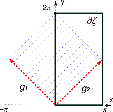
Figure 2: (Color online) Brillouin zone sketched using coordinates $x=k_{x}a/2$ and $y=\sqrt{3}k_{y}a/2$. Primitive reciprocal lattice vectors ${\bf G}_{1}=(2\pi/a)(1,1/\sqrt{3})$ and ${\bf G}_{2}=(2\pi/a)(-1,1/\sqrt{3})$ correspond to ${\bf g}_{1}=(\pi,\pi)$ and ${\bf g}_{2}=(-\pi,\pi)$ respectively. The black rectangle marks the boundary $\partial\zeta$ of the zone used for polarization calculations in Sec. VI.

Since, $\hat{\theta}\Gamma^{\alpha}\hat{\theta}^{-1}=\Gamma^{\alpha}$ and $\hat{\theta}\Gamma^{\alpha\beta}\hat{\theta}^{-1}=-\Gamma^{\alpha\beta}$, while $d_{\alpha}({\bf k})=d_{\alpha}(-{\bf k})$ and $d_{\alpha\beta}({\bf k})=-d_{\alpha\beta}(-{\bf k})$, the Hamiltonian (9) is time-reversal invariant, i.e., $\hat{\theta}H({\bf k})\hat{\theta}^{-1}=H(-{\bf k})$. However, it lacks particle-hole symmetry in the sense of Refs. (Schnyder-PRB08, ; Schnyder-AIP09, ; Kitaev-AIP09, ), because of the action of the on-site and spin-orbit coupling terms. In the general classification of topological insulators and superconductors,Schnyder-PRB08 ; Schnyder-AIP09 ; Kitaev-AIP09 therefore, the Kane-Mele model falls into the AII symplectic symmetry class, which in two dimensions has a $\mathbb{Z}_{2}$ classification. This means that by varying parameters of the Hamiltonian of Eq. (9) one can switch between $\mathbb{Z}_{2}$-odd and $\mathbb{Z}_{2}$-even phases, with the system experiencing a gap closure and becoming metallic at the transition from one phase to the other.

For the present purposes we assume $\lambda_{\rm SO}>0$ without loss of generality. We also fix $\lambda_{v}>0$. For this case, the transition between $\mathbb{Z}_{2}$-odd and $\mathbb{Z}_{2}$-even phases is accompanied by a gap closure at the $K$ and $K^{\prime}$ points (the zone-boundary points of three-fold symmetry) in the BZ. The energy is independent of $t$ at these points, and $\lambda_{\rm SO}$ can be used as the energy scale. The energy gap is then given by $|6\sqrt{3}-\lambda_{v}/\lambda_{\rm SO}-\sqrt{(\lambda_{v}/\lambda_{\rm SO})^{2}+9(\lambda_{\rm R}/\lambda_{\rm SO})^{2}}|$, leading to the phase diagram shown in Fig. 3.

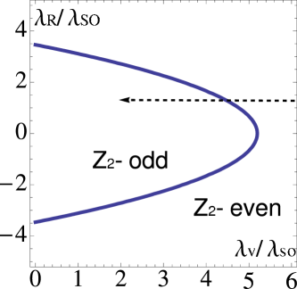
Figure 3: Phase diagram of the Kane-Mele model for $\lambda_{v}/\lambda_{\rm SO}$ $>$ 0. Arrow illustrates a path crossing the phase boundary by varying $\lambda_{v}$ while keeping other parameters fixed.

Note that when $\lambda_{\rm R}=0$ the model reduces to two independent copies of the Haldane modelHaldane-PRL88 the $\mathbb{Z}_{2}$ invariant is odd when the Chern numbers are odd, and even otherwise.Sheng-PRL06

In what follows we use $t$ as the energy scale and fix the values of the other parameters to be $\lambda_{\rm SO}/t=0.6$ and $\lambda_{\rm R}/t=0.5$. Varying the third parameter $\lambda_{v}/t$ allows us to switch from the $\mathbb{Z}_{2}$-even to the $\mathbb{Z}_{2}$-odd phase. The phase transition occurs at $|\lambda_{v}|/t\simeq 2.93$, with the system in the $\mathbb{Z}_{2}$-odd phase for $-2.93<\lambda_{v}/t<2.93$. As discussed above, the energy gap closes at the phase transition, and remains open in both the $\mathbb{Z}_{2}$-odd and $\mathbb{Z}_{2}$-even phases.

IV Gauge freedom and Wannier functions

IV.1 General considerations

We now consider the problem of constructing Wannier functions (WF) for the Kane-Mele model. We emphasize that we mean by this a set of localized functions spanning the same space as the occupied Bloch bands. Several recent papers have discussed the construction of WFs for an enlarged subspace including also some unoccupied bands for 3D topological insulators such as Bi₂Se₃,Zhang-NatPhys09 ; Zhang-NJP10 in which case there is typically no topological obstruction, but this is not the context of the present work.

We start with the general definition of the WF in cell ${\bf R}$ and with band index $n$ in 2D,

$$\langle{\bf r}|{\bf R}n\rangle\equiv W_{n}({\bf r}-{\bf R})=\frac{A}{(2\pi)^{2}}\int_{BZ}d{\bf k}\,e^{-i{\bf k}\cdot{\bf R}}\psi_{n{\bf k}}({\bf r}),$$ (12)

where $A$ is the unit cell area and Bloch wavefunctions $\psi_{n{\bf k}}$ are assumed to be normalized within the unit cell. This definition is not unique; not only is there the usual ${\cal U}(1)$ gauge freedom associated with a $\bf k$-dependent phase twist of each band $n$, there is more generally a ${\cal U}({\cal N})$ gauge freedom

$$|\psi_{n{\bf k}}\rangle\;\longrightarrow\;\sum_{m}U_{mn}({\bf k})\,|\psi_{m{\bf k}}\rangle$$ (13)

coming from the fact that the $\cal N$ occupied Bloch bands can be mixed with each other by a $\bf k$-dependent ${\cal U}({\cal N})$ transformation. In fact, it is generally necessary to pre-mix the Bloch states using this ${\cal U}(N)$ gauge freedom in order that the resulting Bloch-like states (and their phases) will be smooth functions of $\bf k$. However, having done so, there is still a large gauge freedom associated with the application of a subsequent ${\cal U}({\cal N})$ gauge rotation that is smooth in $\bf k$.

This ambiguity in the gauge choice can be removed by applying some criterion to the selection of the WFs. Since electrons are expected to be localized in insulators,Resta-PRL99 a sensible criterion is that of Ref. Marzari-PRB97, , which specifies maximal localization of the WFs in real space. In this approach, which we adopt here, one chooses some localized trial functions in order to provide a starting guess about where the electrons are localized in the unit cell, and obtains a fairly well-localized set of WFs by a projection procedure to be described shortly. If desired, one can follow this with an iterative procedure to make the resulting WFs optimally localized.Marzari-PRB97

Consider an insulator with $\cal N$ occupied bands. We start with a set of $\cal N$ trial states $|\tau_{i}\rangle$ located in the home unit cell, and at each $\bf k$ we project them onto the occupied subspace at $\bf k$ to get a set of Bloch-like states

$$|\Upsilon_{i{\bf k}}\rangle=\hat{P}_{\bf k}\,|\tau_{i}\rangle=\sum_{n=1}^{\cal N}|\psi_{n{\bf k}}\rangle\langle\psi_{n{\bf k}}|\tau_{i}\rangle.$$ (14)

Since this set of states will not generally be orthonormal, we make use of a Löwdin orthonormalization procedure which consists of constructing the overlap matrix

$$S_{mn}({\bf k})=\langle\Upsilon_{m{\bf k}}|\Upsilon_{n{\bf k}}\rangle$$ (15)

and obtaining the orthonormal set of Bloch-like orbitals

$$|\tilde{\psi}_{n{\bf k}}\rangle=\sum_{m}\left[S({\bf k})^{-1/2}\right]_{mn}|\Upsilon_{m{\bf k}}\rangle.$$ (16)

Note that the $\tilde{\psi}_{n{\bf k}}$ are not eigenstates of the Hamiltonian, but they span the same space, and have the same form, as the usual Bloch eigenstates. For an insulator whose gap is not too small, and for a set of trial functions embodying a reasonable assumption about character of the localized electrons, the $\tilde{\psi}_{n{\bf k}}$ will be smooth functions of $\bf k$. In that case, by the usual properties of Fourier transforms, the WFs constructed in analogy with Eq. (12),

$$|{\bf R}n\rangle=\frac{A}{(2\pi)^{2}}\int_{BZ}d{\bf k}\,e^{-i{\bf k}\cdot{\bf R}}\,|\tilde{\psi}_{n{\bf k}}\rangle,$$ (17)

should be well localized.

Such a construction will break down if the determinant of $S({\bf k})$ vanishes at any $\bf k$. This is guaranteed to occur in a Chern insulator, where time-reversal symmetry is broken and the Chern index of the occupied manifold is non-zero; in this case, construction of exponentially localized WFs becomes impossible.Brouder-PRL07 ; Thonhauser-PRB06 ; Thouless-JPC84 For a $\mathbb{Z}_{2}$ insulator, however, the presence of time-reversal symmetry guarantees a zero Chern index, so that exponentially localized WFs must exist.Brouder-PRL07 In this case, we should be able to find a set of trial functions such that ${\rm det}\,S({\bf k})\neq 0$ throughout the BZ.

IV.2 $\mathbb{Z}_{2}$-even phase

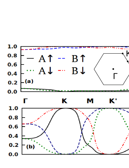
Figure 4: (Color online) Sum of the weights of the projections into the two occupied bands of the basis states $|A;\uparrow_{z}\rangle$, $|B;\uparrow_{z}\rangle$, $|A;\downarrow_{z}\rangle$, and $|B;\downarrow_{z}\rangle$ plotted along the diagonal of the BZ for (a) $\lambda_{v}/t=5$ ($\mathbb{Z}_{2}$-even phase) and (b) $\lambda_{v}/t=1$ ($\mathbb{Z}_{2}$-odd phase). Inset in (a): BZ of a honeycomb lattice.

Let us first apply the method described above to the case of the $\mathbb{Z}_{2}$-even phase of the Kane-Mele model. This phase is topologically equivalent to the ordinary insulator, so we anticipate a picture in which the two electrons per cell are opposite-spin ones approximately localized on the lower-energy ($B$) site. One way to see this is to look at the weights of the basis states in the occupied subspace. Figure 4(a) shows the distribution of these weights along a high-symmetry line in the BZ for the Kane-Mele model in its $\mathbb{Z}_{2}$-even phase. From the figure it is obvious that the two basis states on the $B$ site dominate in the occupied subspace over the whole BZ. It is then natural to choose the two trial functions to be opposite-spin spatial $\delta$-functions localized on the $B$ site in the home unit cell. We choose these to be spin-aligned along $z$, i.e.,

$$|\tau_{i}\rangle=|B;\sigma^{z}_{i}\rangle=\delta({\bf r}-{\bf t}_{B})|\sigma^{z}_{i}\rangle$$ (18)

where $|\sigma^{z}_{1}\rangle=|\!\!\uparrow_{z}\rangle$ and $|\sigma^{z}_{2}\rangle=|\!\!\downarrow_{z}\rangle$. Transforming to ${\bf k}$-space we get

$$|\tau_{i{\bf k}}\rangle=\frac{|\sigma^{z}_{i}\rangle}{\sqrt{N}}\sum_{\bf R}e^{i{\bf k}\cdot{\bf R}}\delta({\bf r}-{\bf R}-{\bf t}_{B}).$$ (19)

The two occupied Bloch bands may be written as

$$|\psi_{n{\bf k}}\rangle=\sum_{\ell}C_{\ell n{\bf k}}|\chi_{\ell{\bf k}}\rangle$$ (20)

where $\ell$ is a combined index for sublattice and spin, $\ell=\{1,2,3,4\}\equiv\{A\uparrow,B\uparrow,A\downarrow,B\downarrow\}$, and $\chi_{\ell{\bf k}}=\chi_{j\sigma{\bf k}}$ are the tight-binding basis functions of Eq. (10). With Eq. (19) the projected functions become

$$|\Upsilon_{1{\bf k}}\rangle=C^{*}_{21{\bf k}}|\psi_{1{\bf k}}\rangle+C^{*}_{22{\bf k}}|\psi_{2{\bf k}}\rangle,$$ (21)

$$|\Upsilon_{2{\bf k}}\rangle=C^{*}_{41{\bf k}}|\psi_{1{\bf k}}\rangle+C^{*}_{42{\bf k}}|\psi_{2{\bf k}}\rangle.$$ (22)

The overlap matrix $S$ is constructed from these functions, and for the determinant one finds

$$\det{[S({\bf k})]} = (|C_{21{\bf k}}|^{2}+|C_{22{\bf k}}|^{2})(|C_{41{\bf k}}|^{2}+|C_{42{\bf k}}|^{2})$$ (23)

$$- |C_{21{\bf k}}C_{41{\bf k}}^{*}+C_{22{\bf k}}C_{42{\bf k}}^{*}|^{2}.$$

Recall that for the Löwdin orthonormalization procedure to succeed, this determinant must remain non-zero everywhere in the BZ. This is indeed the case for the $\mathbb{Z}_{2}$-even phase, as illustrated in Fig. 5(a), where the solid black curve shows the dependence of the determinant on ${\bf k}$ along the high-symmetry line in the BZ.

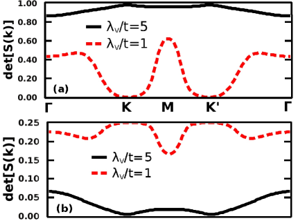
Figure 5: (Color online) Plot of $\det[S({\bf k})]$ along the diagonal of the BZ for $\lambda_{v}/t=5$ ($\mathbb{Z}_{2}$-even phase) and $\lambda_{v}/t=1$ ($\mathbb{Z}_{2}$-odd phase). (a) Trial functions are $|B;\uparrow_{z}\rangle$ and $|B;\downarrow_{z}\rangle$. (b) Trial functions are $|A;\uparrow_{x}\rangle$ and $|B;\downarrow_{x}\rangle$.

In contrast, the dashed red curve in Fig. 5(a) shows the behavior of $\det{[S({\bf k})]}$ in the $\mathbb{Z}_{2}$-odd regime. The determinant can be seen to vanish at the $K$ and $K^{\prime}$ points in the BZ. Clearly, this choice of trial functions is not appropriate for building the Wannier representation in the $\mathbb{Z}_{2}$-odd phase. Indeed, as we shall see in the next subsection, any choice of trial functions that come in Kramers pairs is guaranteed to fail in the $\mathbb{Z}_{2}$-odd case. There we shall also investigate alternative choices of trial functions that allow for a successful construction of WFs.

IV.3 $\mathbb{Z}_{2}$-odd phase

To gain some insight into the appropriate choice of trial functions in the $\mathbb{Z}_{2}$-odd regime, consider the weights of the basis functions in the occupied space shown for this case in Fig. 4(b). Unlike the normal insulator, the $\mathbb{Z}_{2}$-odd phase does not favor any particular basis states. Instead, different basis states dominate in different portions of the BZ. For example, at points $K$ and $K^{\prime}$ the occupied space is represented by only two of the four basis states; at each of these points the two participating basis states have opposite spin and sublattice indices, and none appear in common at both points. (The states at $K$ are, of course, Kramers pairs of those at $K^{\prime}$.) It follows that if any of the trial states is simply set equal to one of the four basis states, then at least one of the $|\Upsilon\rangle$ would vanish either at $K$ or $K^{\prime}$, and the determinant would vanish there too. This explains the failure of the naive Wannier construction procedure for the $\mathbb{Z}_{2}$-odd phase; with the naive choice of trial functions as in Eq. (18), the determinant vanishes at both $K$ and $K^{\prime}$, as shown by the red dashed curve in Fig. 5(a).

In fact, this failure can be understood from a general point of view. If the two trial functions form a Kramers pair, then the projection procedure of Eqs. (14-16) will result in Bloch-like functions obeying

$$|\tilde{\psi}_{1}(-{\bf k})\rangle=\theta|\tilde{\psi}_{2}({\bf k})\rangle,$$

$$|\tilde{\psi}_{2}(-{\bf k})\rangle=-\theta|\tilde{\psi}_{1}({\bf k})\rangle.$$ (24)

The WFs obtained from Eq. (17) will then also form a Kramers pair. But Eq. (24) is nothing other than the constraint of Eq. (5) defining a gauge that respects time-reversal symmetry, and it has been shown Fu-PRB06 ; Roy-PRB09-a ; Loring-arx10 that an odd value of the $\mathbb{Z}_{2}$ invariant presents an obstruction against constructing such a gauge. In other words, in the $\mathbb{Z}_{2}$-odd phase a smooth gauge cannot be fixed by choosing trial functions that are time-reversal pairs of each other, and a choice of WFs as time-reversal pairs is not possible. Hence, in order to construct the Wannier representation in the $\mathbb{Z}_{2}$-odd regime, one should choose trial functions that do not transform into one another under time reversal.

Following these arguments, we choose the two trial functions to be localized on different sites in the home unit cell. Moreover, in order that they will have components on states with spins both up and down along $z$, we choose the spins of the trial states so that one is along $+x$ and the other along $-x$. In $\bf k$-space this becomes

$$|\tau_{i\bf k}\rangle=\frac{|\sigma^{x}_{i}\rangle}{\sqrt{N}}\sum_{\bf R}e^{i{\bf k}\cdot{\bf R}}\delta({\bf r}-{\bf R}-{\bf t}_{i})$$ (25)

where ${\bf t}_{1}={\bf t}_{A}$ and ${\bf t}_{2}={\bf t}_{B}$, leading to

$$|\Upsilon_{1{\bf k}}\rangle=\left[(C_{11{\bf k}}^{*}+C_{31{\bf k}}^{*})|\psi_{1}\rangle+(C_{12{\bf k}}^{*}+C_{32{\bf k}}^{*})|\psi_{2}\rangle\right]/{\sqrt{2}}$$ (26)

and

$$|\Upsilon_{2{\bf k}}\rangle=\left[(C_{21{\bf k}}^{*}-C_{41{\bf k}}^{*})|\psi_{1}\rangle+(C_{22{\bf k}}^{*}-C_{42{\bf k}}^{*})|\psi_{2}\rangle\right]/{\sqrt{2}}.$$ (27)

The determinant takes the form

$$\det[S] = (|C_{11{\bf k}}+C_{31{\bf k}}|^{2}+|C_{12{\bf k}}+C_{32{\bf k}}|^{2})(|C_{21{\bf k}}-C_{41{\bf k}}|^{2}+|C_{22{\bf k}}-C_{42{\bf k}}|^{2})/4-$$ (28)

$$- |(C_{11{\bf k}}+C_{31{\bf k}})(C_{21{\bf k}}^{*}-C_{41{\bf k}}^{*})+(C_{12{\bf k}}+C_{32{\bf k}})(C_{22{\bf k}}^{*}-C_{42{\bf k}}^{*})|^{2}/4.$$

The dependence $\det[S({\bf k})]$ is shown along the diagonal of the Brillouin zone for this choice of trial functions in Fig. 5(b). In the $\mathbb{Z}_{2}$-odd phase (dashed line) the determinant remains non-zero everywhere in the BZ. Not surprisingly, the same trial functions are very poorly suited to the normal-insulator phase, as can be seen from solid line in the same panel. In this case $\det[S({\bf k})]$ almost vanishes at $K$ and $K^{\prime}$ and remains quite small throughout the rest of the BZ, so that one should clearly revert to the time-reversed pair of trial functions of Eq. (18) and Fig. 5(a) in order to get well-localized WFs.

We made an arbitrary choice above in selecting the two trial functions to be up and down along $x$. In fact, if we repeat the entire procedure using trial functions that are spin-up and spin-down along any unit vector $\hat{n}$ lying in the $xy$-plane, we find that $\det[S({\bf k})]$ changes very little, with only small changes in the size of the dip near the $\Gamma$ point. Thus, we find that the choice of trial functions in Eq. (25) is not unique. Instead, there is a large degree of arbitrariness in the choice of WFs in the $\mathbb{Z}_{2}$-odd case.

To conclude, we have established that the choice of a time-reversal pair of trial functions, Eq. (18), that allows for the construction of well-localized WFs in the ordinary-insulator phase cannot be used in the $\mathbb{Z}_{2}$-odd phase. In order for the usual projection method for constructing the Wannier representation to work in this topologically nontrivial phase, the trial functions should explicitly break time-reversal symmetry, i.e., they should not come in time-reversal pairs.

V Localization of Wannier Functions in the $\mathbb{Z}_{2}$-odd Insulator

Now that we know how to construct WFs for the $\mathbb{Z}_{2}$-odd insulator, we discuss their localization properties. As we have noted in the preceding section, the choice of the trial functions, Eq. (25), is not unique; there are other gauge choices arising from different trial functions that also produce well-defined sets of WFs. Since different gauge choices lead to different degrees of localization of the resulting WFs, it is natural to fix the gauge by the condition of maximal possible localization of the WFs.

The problem of constructing maximally-localized WFs was studied by Marzari and Vanderbilt.Marzari-PRB97 They considered the total quadratic spread

$$\Omega=\sum_{n=1}^{\cal N}[\langle{\bf 0}n|r^{2}|{\bf 0}n\rangle-\langle{\bf 0}n|{\bf r}|{\bf 0}n\rangle^{2}]$$ (29)

as a measure of the delocalization of WFs in real space, and developed methods for iteratively reducing the spread via a series of unitary transformations, Eq. (13), applied prior to WF construction. The spread functional was decomposed into two parts, $\Omega=\Omega_{I}+\tilde{\Omega}$, with

$$\Omega_{I}=\sum_{n=1}^{\cal N}\left[\langle{\bf 0}n|r^{2}|{\bf 0}n\rangle-\sum_{{\bf R}m}|\langle{\bf R}m|{\bf r}|{\bf 0}n\rangle|^{2}\right]$$ (30)

being the gauge-invariant part and

$$\tilde{\Omega}=\sum_{n=1}^{{\cal N}}\sum_{{\bf R}m\neq{\bf 0}n}|\langle{\bf R}m|{\bf r}|{\bf 0}n\rangle|^{2}$$ (31)

the gauge-dependent part of the spread. Discretized ${\bf k}$-space formulas for Eqs. (30) and (31) were also derived for the case that the BZ is represented by a uniform $\bf k$ mesh. The resulting expression for the gauge-invariant spread is, for example,

$$\Omega_{I}=\frac{1}{N}\sum_{{\bf k},{\bf b}}\omega_{b}\sum_{m,n=1}^{\cal N}\left(\delta_{mn}-|M_{mn}^{({\bf k},{\bf k}+{\bf b})}|^{2}\right),$$ (32)

where

$$M_{mn}^{({\bf k},{\bf k}+{\bf b})}=\langle u_{n{\bf k}}|u_{m{\bf k}+{\bf b}}\rangle=\sum_{\ell=1}^{4}C_{\ell n{\bf k}}^{*}C_{\ell m{\bf k}+{\bf b}}e^{-i{\bf b}\cdot{\bf t}_{\ell}}$$ (33)

are overlap matrices and ${\bf b}$ are “mesh vectors” connecting each ${\bf k}$-point to its nearest neighbors. The latter are chosen, together with a set of weights $\omega_{b}$, in such a way as to satisfy the condition

$$\sum_{\bf b}\omega_{b}b_{i}b_{j}=\delta_{ij}.$$ (34)

A corresponding expression for $\tilde{\Omega}$, and a description of steepest-descent methods capable of minimizing $\Omega$, were also given in Ref. Marzari-PRB97, . Note that, in order to avoid getting trapped in false local minima, the iterative procedure is normally initialized using the trial-function projection procedure described in Sec. IV above.

We now apply this method to the Kane-Mele model. The lattice is hexagonal, and in this case six ${\bf b}_{j}$ vectors are needed to satisfy the condition (34), namely ${\bf b}_{1}=-{\bf b}_{4}={\bf G}_{1}/q$, ${\bf b}_{2}=-{\bf b}_{5}=({\bf G}_{1}+{\bf G}_{2})/q$, and ${\bf b}_{3}=-{\bf b}_{6}={\bf G}_{2}/q$. All six have the same length $b$ and weight $\omega_{b}=1/(3b^{2})$. We start with the WFs obtained with the projection method using the trial functions of Eq. (25), appropriate for the $\mathbb{Z}_{2}$-odd phase.

The resulting spreads, both before and after the iterative minimization, are shown in Fig. 6.

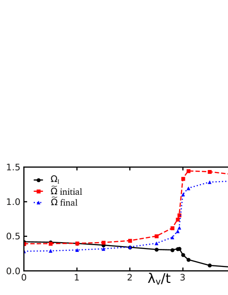
Figure 6: (Color online) Wannier spreads $\Omega_{I}$ and $\tilde{\Omega}$ for the Kane-Mele model on a 60$\times$60 ${\bf k}$-mesh, initialized using the trial functions of Eq. (25). “Initial” and “final” values are those computed before and after the iterative minimization respectively. The system is in the $\mathbb{Z}_{2}$-odd phase for $\lambda_{v}/t\lesssim 2.93$.

($\Omega_{I}$, being gauge-invariant, is the same before and after.) The left part of the figure shows the behavior in the $\mathbb{Z}_{2}$-odd phase, where the trail functions are the appropriate ones. The results in this region were not strongly sensitive to the $\bf k$-point mesh density. The fact that $\tilde{\Omega}$ is similar in magnitude to the unminimized $\Omega_{I}$, and that the localization procedure reduces $\tilde{\Omega}$ by only $20-30\%$, provide additional evidence that the choice of trial functions was a good one. The Wannier charge centers were almost unchanged by the minimization procedure; the $x$-coordinates were zero, while $\bar{r}_{1y}\simeq a/\sqrt{3}$ and $\bar{r}_{2y}\simeq 2a/\sqrt{3}$ (see Sec. VI for details), in good agreement with our initial assumption about the WFs being localized on $A$ and $B$ sites.

The right part of Fig. 6, for $\lambda_{v}/t\gtrsim 2.93$, shows what happens when we attempt to use the same trial functions in the normal phase. $\Omega_{I}$ is of course unaffected by the choice of trial functions, and the fact that it has a smaller value in this region indicates, not surprisingly, that the insulating state is simpler and more localized in the normal state. (For large $\lambda_{v}/t$ the WFs approach spatial delta functions, explaining the fact that $\Omega_{I}$ asymptotes to zero in that limit.) Not surprisingly, however, using the trial functions appropriate to the $\mathbb{Z}_{2}$-odd phase in the $\mathbb{Z}_{2}$-even regime results in very poor localization of the WFs as measured by $\tilde{\Omega}$. Our data also suggests that in the $\mathbb{Z}_{2}$-odd phase MLWFs are less localized than MLWS in the $\mathbb{Z}_{2}$-even phase. For example, the use of trial functions (18) with $\lambda_{v}/t=5$ and a $60\times 60$ ${\bf k}$-mesh results in $\Omega_{I}=0.02770$ and $\tilde{\Omega}=0.00025$. We also find that the results are more sensitive to the choice of $\bf k$-mesh in the $\mathbb{Z}_{2}$-odd regime.

To summarize the results of this section, we studied the construction of maximally localized WFs in the $\mathbb{Z}_{2}$-odd phase using the Kane-Mele model as an example. We have seen that our initial guess of Sec. IV about the localization of WFs in this topological regime is very good, and that the maximal localization procedure does not greatly reduce the spread.

VI Hybrid Wannier charge centers and polarization

In this section we discuss the polarization in $\mathbb{Z}_{2}$-odd insulators using the example of the Kane-Mele model, and see what insights about the topological insulating phase can be obtained by inspecting this property.

The electronic polarization in a 2D system can be defined either in terms of the Berry phaseKing-Smith-PRB93

$${\bf P}=\frac{|e|}{(2\pi)^{2}}\mathrm{Im}\sum_{n=1}^{\cal N}\int d{\bf k}\langle u_{n{\bf k}}|\nabla_{\bf k}|u_{n{\bf k}}\rangle$$ (35)

or via the summation of Wannier charge centersVanderbilt-PRB93

$${\bf P}=-\,\frac{|e|}{A}\sum_{n=1}^{\cal N}\bar{\bf r}_{n},$$ (36)

where $e$ is the electronic charge and $A$ is the area of the unit cell. The two definitions are identical and define electronic polarization modulo a polarization quantum $|e|{\bf R}/A$, ${\bf R}$ being a lattice vector. This ambiguity can be understood as a freedom in the choice of branch in Eq. (35) or in the choice of unit cell in Eq. (36). The definition via Wannier charge centers makes the dependence of $\bf P$ on the choice of origin obvious. As described in Sec. III, the origin of the Kane-Mele model is chosen such that atoms are located along the $y$-axis at ${\bf t}_{A}=\xi\hat{y}/3$ and ${\bf t}_{B}=2\xi\hat{y}/3$, where $\xi=|{\bf a}_{1}+{\bf a}_{2}|=a\sqrt{3}$. Because the Hamiltonian has 3-fold symmetry, we expect the rescaled polarization $(A/|e|)\bf P$ to lie at the origin, at ${\bf t}_{A}$, or at ${\bf t}_{B}$. To distinguish between these possibilities it is sufficient to compute $P_{y}$, which is well-defined modulo $|e|/a$.

VI.1 Total polarization

A direct computation of electronic polarization via Eq. (35) in the $\mathbb{Z}_{2}$-even phase results in $P_{y}=|e|/3a$ mod $|e|/a$, consistent with the fact that both Wannier centers in Eq. (36) lie at ${\bf t}_{B}$ (since $-4|e|\xi/3A=-8|e|/3a=|e|/3a$ mod $|e|/a$.) In the $\mathbb{Z}_{2}$-odd phase, on the other hand, Eqs. (35) and (36) lead to $P_{y}=0$ mod $|e|/a$. Again, this is consistent with the locations of the WFs. As indicated in Sec. V, the Wannier centers $\bar{\bf r}_{n}$ in this phase lie approximately at ${\bf t}_{A}$ and ${\bf t}_{B}$. More precisely, we find that they are located at $\bar{\bf r}_{1}=(1-\delta)\xi\hat{y}/3$ and $\bar{\bf r}_{2}=(2+\delta)\xi\hat{y}/3$, where $\delta$ is a small correction (e.g., $\delta=0.0018$ at $\lambda_{v}/t=1$). Thus, the sum of the Wannier centers is just $\xi\hat{y}$, or zero modulo a lattice vector.

It is interesting to note that, in retrospect, the computation of the polarization via Eq. (35) would have given a strong hint about the appropriate choice of trial functions in the $\mathbb{Z}_{2}$-odd insulator. That is, knowing only that $P_{y}=0$, one might have guessed that both WFs should be centered halfway between ${\bf t}_{A}$ and ${\bf t}_{B}$, or both at the center of the honeycomb ring, or one at ${\bf t}_{A}$ and the other at ${\bf t}_{B}$. The latter possibility becomes the most likely when we also take into account that in the $\mathbb{Z}_{2}$-odd phase the two WFs cannot form a Kramers pair.

VI.2 Hybrid Wannier decomposition

In order to obtain a deeper understanding of the origin of the polarization and expose some qualitative differences in the behavior of its ${\bf k}$-dependent decomposition in $\mathbb{Z}_{2}$-even and odd phases, it is useful to use a hybrid representation in which the Wannier transformation is carried out in one direction only. As indicated above, we know from symmetry considerations that we can set $P_{x}=0$ and characterize the polarization by $P_{y}$ mod $\xi|e|/A$. To compute $P_{y}$, it is convenient to choose the BZ to be a rectangle extending over $k_{x}\in[0,2\pi/a]$ and $k_{y}\in[0,4\pi/\xi]$ (corresponding to the region $\zeta$ in Fig. 2). We can then define hybrid WFs

$$|nk_{x}l_{y}\rangle=\frac{\xi}{4\pi}\int_{0}^{4\pi/\xi}dk_{y}\,e^{-ik_{y}l_{y}}|\tilde{\psi}_{n{\bf k}}\rangle$$ (37)

in terms of which the usual WFs are

$$|{\bf R}n\rangle=|nl_{x}l_{y}\rangle=\frac{a}{2\pi}\int_{0}^{2\pi/a}dk_{x}\,e^{-ik_{x}l_{x}}|nk_{x}l_{y}\rangle.$$ (38)

The hybrid Wannier centers are defined as

$${\bar{y}_{n}(k_{x})}=\langle nk_{x}0|y|nk_{x}0\rangle$$ (39)

and the total electronic polarization is

$$P_{y}=-\frac{|e|}{\pi\xi}\sum_{n}\int_{0}^{2\pi/a}dk_{x}\,{\bar{y}_{n}(k_{x})}.$$ (40)

In practice the $k_{x}$ integral is discretized by a sum over a mesh of $k_{x}$ values, and at each $k_{x}$ the ${\bar{y}_{n}(k_{x})}$ are calculated by considering the corresponding string of $\bf k$-points along $k_{y}$. In the case that the gauge has been specified by a particular set of 2D WFs $|{\bf R}n\rangle$, or, equivalently, by the corresponding Bloch-like functions $|\tilde{\psi}_{n\bf k}\rangle$, this is done straightforwardly using the discretized Berry-phase formula

$${\bar{y}_{n}(k_{x})}=-\frac{\xi}{4\pi}\,\mathrm{Im}\log\prod_{j}M^{(j)}_{nn}$$ (41)

where $M^{(j)}$ is a shorthand for the overlap matrix $M^{({\bf k}_{j},{\bf k}_{j+1})}$ of Eq. (33) connecting $k_{y}$-points $j$ and $j+1$ along the string.

As was emphasized in Sec. IV, the $\tilde{\psi}_{n{\bf k}}$ carry the information about the gauge choice. Thus, different gauge choices – i.e., different choices of WFs – will result in different hybrid WFs and different ${\bar{y}_{n}(k_{x})}$. However, the sum $\sum_{n}{\bar{y}_{n}(k_{x})}$ at a given $k_{x}$ is gauge-invariant, and as a result $P_{y}$ of Eq. (40) must remain the same in any gauge.

Of special interest is a gauge choice in which, at each $k_{x}$, the hybrid WFs $|nk_{x}l_{y}\rangle$ are maximally localized in the $y$ direction. It was shown in Ref. Marzari-PRB97, that in 1D the Wannier charge centers can be obtained by a parallel-transport construction using the overlap matrices $M^{(j)}$. Specifically, the “unitary part” $\widetilde{M}^{(j)}$ of each overlap matrix is obtained by carrying out the singular-value decomposition $M=V\Sigma W^{\dagger}$, where $V$ and $W$ are unitary and $\Sigma$ is real-positive and diagonal, and then setting $\widetilde{M}=VW^{\dagger}$. This is reasonable because, for a sufficiently fine mesh spacing, $\Sigma$ is almost the unit matrix. Then, the unitary matrix $\Lambda=\prod_{j}\widetilde{M}^{(j)}$ describes the transport of states along the string. The eigenvalues $\lambda_{n}$ of this matrix are all of unit modulus, and their phases define Wannier centers viaWu-PRL06

$${\bar{y}_{n}(k_{x})}=-\frac{\xi}{4\pi}\mathrm{Im}\log{\lambda_{n}}.$$ (42)

Note that no iterative procedure is needed. Inserting this equation into Eq. (40), one gets a discretized formula for $P_{y}$ that is consistent with Eq. (35).

VI.3 Results

We illustrate these ideas now for the KM model in its normal and $\mathbb{Z}_{2}$-odd phases. In each case we present results for ${\bar{y}_{n}(k_{x})}$ for two choices of gauge: the maximally-localized one along $\hat{y}$ as discussed in the previous paragraph, and the one corresponding to the WFs constructed from the trial functions of Eq. (18) for the $\mathbb{Z}_{2}$-even phase or those of Eq. (25) for the $\mathbb{Z}_{2}$-odd phase. In what follows, we refer to these as the “maxloc” and “WF-based” gauges respectively.

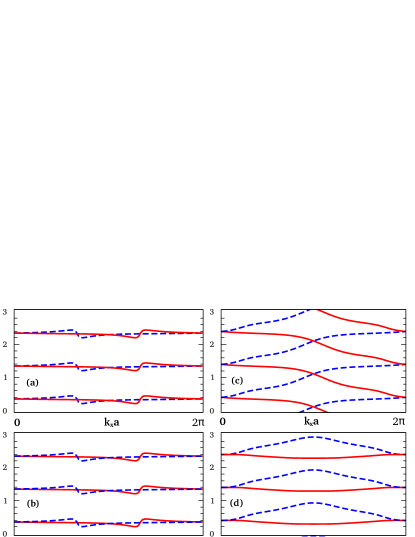
Figure 7: (Color online) Hybrid Wannier centers ${\bar{y}_{n}(k_{x})}$, in units of $\xi/2$, for the Kane-Mele model. $\mathbb{Z}_{2}$-even phase ($\lambda_{v}/t=3$): (a) maxloc gauge; (b) WF gauge of Eq. (18). $\mathbb{Z}_{2}$-odd phase ($\lambda_{v}/t=1$): (c) maxloc gauge; (d) WF gauge of Eq. (25). In each case, several periodic images are shown.

In the ordinary insulating regime, the maxloc and WF-based ${\bar{y}_{n}(k_{x})}$ curves look very similar to each other. Fig. 7(a) and (b) show the calculated results for the case of $\lambda_{v}/t=3$, very close to the transition on the insulating side (recall the critical value is at $\lambda_{v}/t=2.93$). Three of the infinite number of periodic images along $y$ are shown. The “bumps” in the curves near the $K$ and $K^{\prime}$ points in the BZ are the result of the proximity to the transition; as one goes deeper into the insulating phase, the curves flatten out and become smooth functions of $k_{x}$. The solid and dashed curves are mirror images of each other; in the maxloc construction of Fig. 7(a) this just reflects the time-reversal invariance of the Hamiltonian, while in Fig. 7(b) it follows from the fact that the WFs form a Kramers pair.

When averaged over $k_{x}$, each curve is found to have a mean $\bar{y}$ value of $2\xi/3$ to numerical precision, or $\xi/6$ modulo $\xi/2$, consistent with the discussion in Sec. VI.1.

The corresponding results for the $\mathbb{Z}_{2}$-odd phase are shown in Fig. 7(c) and (d) for $\lambda_{v}/t=1$. As expected, there is again a mirror symmetry visible in the curves for the maxloc construction in Fig. 7(c), but the connectivity of the curves is qualitatively different: in going from $k_{x}=0$ to $\pi/a$ we see that the $n$’th solid curve goes up to cross the $(n+1)$’th dashed curve, while the $n$’th dashed curve goes down to cross the $(n-1)$’th solid curve. This is exactly the kind of behavior that was exhibited in Fig. 3(a) of Ref. Fu-PRB06, as a signal of the $\mathbb{Z}_{2}$-odd phase. Moreover, if we follow the $n$’th dashed curve all the way across the BZ, we find that it wraps to become the $(n+1)$’th one when $k_{x}=2\pi/a$ wraps back to $k_{x}=0$. This is precisely the kind of behavior that is characteristic of a Chern (or quantum anomalous Hall) insulator,Coh-PRL09 which implies that we can assign a Chern number of $+1$ to the Bloch subspace spanned by the eigenvectors corresponding to the dashed bands. However, since we are studying here a system with time-reversal symmetry, we find also a partner subspace corresponding to the full curve in Fig. 7(c) having Chern number $-1$. As a result, of course, the overall occupied space has a total vanishing Chern number, as it must due to the time-reversal symmetry. The evaluation of the polarization $P_{y}$ through Eq. (40) again yields $P_{y}=0$ mod $|e|/a$, consistent with the direct calculation of Sec. VI.1.

Finally, Fig. 7(d) shows the ${\bar{y}_{n}(k_{x})}$ curves for the same $\mathbb{Z}_{2}$-odd parameters as in Fig. 7(c), but using the WF-based gauge determined by the trial functions of Eq. (25). At any given $k_{x}$, we confirm that $\bar{y}_{1}+\bar{y}_{2}$ is the same in Fig. 7(d) as in Fig. 7(c), and the total polarization is therefore the same. However, because the two WFs do not form a Kramers pair in this case, the dashed and solid curves do not map into each other under time-reversal symmetry, and there is no degeneracy at $k_{x}=\pi/a$. Moreover, the Chern number of each band is individually zero, consistent with the fact that each one is derived from a WF. The average $\bar{y}$ values for the solid and dashed curves are $0.978\xi/3$ and $2.022\xi/3$ mod $\xi/2$, very close to the nominal locations of the trial functions at ${\bf t}_{A}$ and ${\bf t}_{B}$, respectively.

To recap, in both the $\mathbb{Z}_{2}$-even and $\mathbb{Z}_{2}$-odd cases, we find that the occupied Bloch space can be cast as the direct sum of two subspaces that map into one another under the time-reversal operation, corresponding to the solid and dashed curves of Figs. 7(a-c). These subspaces are not built from Hamiltonian eigenstates, but from suitable $\bf k$-dependent ${\cal U}(2)$ rotations among the Hamiltonian eigenstates. In the $\mathbb{Z}_{2}$-even case the Chern index of each of these subspaces is separately zero, so that we can also provide a Wannier representation for each subspace separately. This is essentially the case of Fig. 7(b), and since the spaces form a time-reversal pair, the WFs form a time-reversal pair as well. In contrast, for the $\mathbb{Z}_{2}$-odd phase, the decomposition into two subspaces that are time-reversal images of each other necessarily results in subspaces having individual Chern numbers of $\pm$1, and these are not individually Wannier-representable. Only by violating the condition that the two spaces be time-reversal partners, as was done in Fig. 7(d), can we decompose the space into two subspaces having zero Chern indices individually. By doing so, we can find a Wannier representation of the entire space, but only on condition that the two WFs do not form a Kramers pair.

VII Conclusions

In this paper we have considered the question of how to construct a Wannier representation for $\mathbb{Z}_{2}$-odd topological insulators in 2D. We have shown that the usual method based on projection onto trial functions fails because of a topological obstruction if one imposes the condition that the trial functions should come in time-reversal pairs. On the other hand, the projection method can be made to work if this condition is not imposed, resulting in WFs that do not transform into one another under time reversal.

Such a Wannier representation may have some formal disadvantages. For example, if one writes the Hamiltonian as a matrix in this Wannier representation, its time-reversal invariance is no longer transparent, and the presence of other symmetries may become less obvious as well. On the other hand, it does satisfy all the usual properties of a Wannier representation, as for example the ability to express the electric polarization in terms of the locations of the Wannier centers, and there is every reason to expect that the maximally localized WFs are still exponentially localized. Brouder-PRL07

The generalization of our findings to the 3D case should be relatively straightforward. Certainly the topological obstruction to the construction of Kramers-pair WFs remains for both weak and strong $\mathbb{Z}_{2}$ topological insulators in 3D. To see this, consider in turn each of the six symmetry planes in $\bf k$-space ($k_{1}=0$, $k_{2}=0$, $k_{3}=0$, $k_{1}=\pi/a$, etc.) on which $H_{\bf k}$ behaves like a 2D time-reversal invariant system. For both weak and strong topological insulators, at least one of these six planes must have a $\mathbb{Z}_{2}$-odd 2D invariant. But if a gauge exists obeying the time-reversal condition of Eq. (5) in the 3D $\bf k$-space, then it does so in particular on the 2D plane, in contradiction with the 2D arguments about a topological construction.

Thus, the general strategy for constructing WFs for 3D topological insulators should be very similar to the one presented here in 2D. Namely, one has to choose pairs of trial functions that do not transform into one another by time-reversal symmetry, and to do it in such a way that the projection of these trial functions onto the Bloch states does not become singular anywhere in the 3D BZ. While it may be interesting to explore how this might best be done in practice for real 3D topological insulators, e.g., in the density-functional context, the choice is likely to depend sensitively on details of the particular system of interest. Thus, an investigation of these issues falls beyond the scope of the present work.

VIII Acknowledgments

The work was supported by NSF Grant DMR-0549198.

References

- (1) A. P. Schnyder, S. Ryu, A. Furusaki, and A. W. W. Ludwig, Phys. Rev. B 78, 195125 (2008)
- (2) A. P. Schnyder, S. Ryu, A. Furusaki, and A. W. W. Ludwig, AIP Conf. Proc. 1134, 10 (2009)
- (3) A. Kitaev, AIP Conf. Proc. 1134, 22 (2009)
- (4) D. J. Thouless, M. Kohmoto, M. P. Nightingale, and M. den Nijs, Phys. Rev. Lett. 49, 405 (1982)
- (5) F. D. M. Haldane, Phys. Rev. Lett. 61, 2015 (1988)
- (6) C. L. Kane and E. J. Mele, Phys. Rev. Lett. 95, 146802 (2005)
- (7) B. A. Bernevig, T. L. Hughes, and S.-C. Zhang, Science 314, 1757 (2006)
- (8) H. Zhang, C.-X. Liu, X.-L. Qi, X. Dai, Z. Fang, and S.-C. Zhang, Nat. Phys. 5, 438 (2009)
- (9) L. Fu and C. L. Kane, Phys. Rev. B 76, 045302 (2007)
- (10) M. Konig, S. Wiedmann, C. Brune, A. Roth, H. Buhmann, L. W. Molenkamp, X.-L. Qi, and S.-C. Zhang, Science 318, 766 (2007)
- (11) Y. L. Chen, J. G. Analytis, J.-H. Chu, Z. K. Liu, S.-K. Mo, X. L. Qi, H. J. Zhang, D. H. Lu, X. Dai, Z. Fang, S. C. Zhang, I. R. Fisher, Z. Hussain, and Z.-X. Shen, Science 325, 178 (2009)
- (12) D. Hsieh, D. Qian, L. Wray, Y. Xia, Y. S. Hor, R. J. Cava, and M. Z. Hasan, Nature 452, 970 (2008)
- (13) D. Hsieh, Y. Xia, L. Wray, D. Qian, A. Pal, J. H. Dil, J. Osterwalder, F. Meier, G. Bihlmayer, C. L. Kane, Y. S. Hor, R. J. Cava, and M. Z. Hasan, Science 323, 919 (2009)
- (14) Y. Xia, D. Qian, D. Hsieh, L. Wray, A. Pal, H. Lin, A. Bansil, D. Grauer, Y. S. Hor, R. J. Cava, and M. Z. Hasan, Nat. Phys. 5, 398 (2009)
- (15) J. E. Moore and L. Balents, Phys. Rev. B 75, 121306 (2007)
- (16) L. Fu, C. L. Kane, and E. J. Mele, Phys. Rev. Lett. 98, 106803 (2007)
- (17) N. Marzari and D. Vanderbilt, Phys. Rev. B 56, 12847 (1997)
- (18) D. Vanderbilt and R. D. King-Smith, Phys. Rev. B 48, 4442 (1993)
- (19) T. Thonhauser and D. Vanderbilt, Phys. Rev. B 74, 235111 (2006)
- (20) D. J. Thouless, J. Phys. C 17, L325 (1984)
- (21) C. Brouder, G. Panati, M. Calandra, C. Mourougane, and N. Marzari, Phys. Rev. Lett. 98, 046402 (2007)
- (22) C. L. Kane and E. J. Mele, Phys. Rev. Lett. 95, 226801 (2005)
- (23) L. Fu and C. L. Kane, Phys. Rev. B 74, 195312 (2006)
- (24) M. V. Berry, Proc. R. Soc. Lon. A 392, 45 (1984)
- (25) T. Fukui and Y. Hatsugai, J. Phys. Soc. Jpn. 76, 053702 (2007)
- (26) Y. Bychkov and E. Rashba, JETP Lett. 39, 78 (1984)
- (27) An alternative tight-binding convention, defined by replacing by in Eq. (10), is possible but is not adopted here.
- (28) D. N. Sheng, Z. Y. Weng, L. Sheng, and F. D. M. Haldane, Phys. Rev. Lett. 97, 036808 (2006)
- (29) W. Zhang, R. Yu, H.-J. Zhang, X. Dai, and Z. Fang, New J. of Phys. 12, 065013 (2010)
- (30) R. Resta and S. Sorella, Phys. Rev. Lett. 82, 370 (1999)
- (31) Fig. 4(b) also shows that the character of the occupied states changes in the BZ, which serves as an illustration of the band inversion associated with topological insulators.
- (32) R. Roy, Phys. Rev. B 79, 195321 (2009)
- (33) T. A. Loring and M. B. Hastings, “Disordered topological insulators via -algebras,” arXiv:1005.4883
- (34) To see that the components have to be mixed, consider two trial functions that are localized on different sites and with opposite direction of spin in the direction. In this case the projected functions become zero either at or , as follows from the Fig. 4(b), and becomes zero.
- (35) Actually, the minimum value of occurs off the plotted symmetry line and is .
- (36) R. D. King-Smith and D. Vanderbilt, Phys. Rev. B 47, 1651 (1993)
- (37) X. Wu, O. Diéguez, K. M. Rabe, and D. Vanderbilt, Phys. Rev. Lett. 97, 107602 (2006)
- (38) S. Coh and D. Vanderbilt, Phys. Rev. Lett. 102, 107603 (2009)