Reconstructing CMEs with Coordinated Imaging and In Situ Observations: Global Structure, Kinematics, and Implications for Space Weather Forecasting

Abstract

We reconstruct the global structure and kinematics of coronal mass ejections (CMEs) using coordinated imaging and in situ observations from multiple vantage points. A forward modeling technique, which assumes a rope-like morphology for CMEs, is used to determine the global structure (including orientation and propagation direction) from coronagraph observations. We reconstruct the corresponding structure from in situ measurements at 1 AU with the Grad-Shafranov (GS) method, which gives the flux-rope orientation, cross section and a rough knowledge of the propagation direction. CME kinematics (propagation direction and radial distance) during the transit from the Sun to 1 AU are studied with a geometric triangulation technique, which provides an unambiguous association between solar observations and in situ signatures; a track fitting approach is invoked when data are available from only one spacecraft. We show how the results obtained from imaging and in situ data can be compared by applying these methods to the 2007 November 14-16 and 2008 December 12 CMEs. This merged imaging and in situ study shows important consequences and implications for CME research as well as space weather forecasting: (1) CME propagation directions can be determined to a relatively good precision as shown by the consistency between different methods; (2) the geometric triangulation technique shows a promising capability to link solar observations with corresponding in situ signatures at 1 AU and to predict CME arrival at the Earth; (3) the flux rope within CMEs, which has the most hazardous southward magnetic field, cannot be imaged at large distances due to expansion; (4) the flux-rope orientation derived from in situ measurements at 1 AU may have a large deviation from that determined by coronagraph image modeling; (5) we find, for the first time, that CMEs undergo a westward migration with respect to the Sun-Earth line at their acceleration phase, which we suggest as a universal feature produced by the magnetic field connecting the Sun and ejecta. Importance of having dedicated spacecraft at L4 and L5, which are well situated for the triangulation concept, is also discussed based on the results.

1 Introduction

Coronal mass ejections (CMEs) are the most spectacular eruptions in the solar corona in which $10^{15-16}$ g of plasma with $10^{31-32}$ ergs of energy is hurled into interplanetary space (e.g., Gosling et al., 1974; Hundhausen, 1997). The ejected materials in the solar wind, a key link between activity at the Sun and disturbances in the heliosphere, are called interplanetary coronal mass ejections (ICMEs). A subset of ICMEs, termed as magnetic clouds (MCs), are characterized by a strong magnetic field, a smooth and coherent rotation of the field, and a depressed proton temperature compared with the ambient solar wind (Burlaga et al., 1981).

CMEs have been recognized as drivers of major space weather effects. They are responsible for the most intense solar energetic particle events, which can endanger life and technology on the Earth and in space. They can also cause major geomagnetic storms in the terrestrial environment including large auroral currents and high particle fluxes, which can disrupt satellite operations, power systems and radio communications. CMEs drive space weather effects typically in two ways. First, CMEs are often associated with a sustained southward magnetic field, which can reconnect with geomagnetic fields and produce storms in the terrestrial environment (Dungey, 1961; Gosling et al., 1991). The southward field component is either within the ejecta or produced by the interaction of the ejecta with the ambient medium (Gosling & McComas, 1987; McComas et al., 1988; Liu et al., 2008a). Second, fast CMEs can generate interplanetary shocks, a key source of energetic particles and radio bursts. Note that the magnetic reconnection rate at the dayside of the magnetopause is controlled by the dawn-dusk electric field, $-\textbf{v}_{r}\times\textbf{B}_{s}$, where $\textbf{v}_{r}$ is the radial velocity of the solar wind and $\textbf{B}_{s}$ is the southward magnetic field component. Therefore, the high speed of CMEs can also significantly enhance the magnetic reconnection rate when a southward magnetic field is present.

CMEs have been studied by remote sensing of these events at the Sun and by in situ measurements of their plasma properties when they encounter spacecraft. However, most CME studies are focused on the phenomena either at the Sun or near the Earth; efforts to link solar and in situ observations, especially the development of practical strategies for space weather forecasting, are still lacking. The global structure of CMEs and the underlying physics governing CME propagation in the heliosphere are not well understood. Remote sensing observations, mostly by coronagraphs, can provide a long warning time in terms of the occurrence and speed of CMEs. Coronagraphs record photospheric radiation (or white light) Thomson-scattered by electrons (Billings, 1966), so what is observed is essentially a density structure projected onto the sky. The magnetic field orientation is difficult to determine directly from white-light observations. It is also a challenge to infer the three-dimensional (3D) structure and kinematics from a single viewpoint due to projection effects. In situ measurements at the first Lagrangian point (L1) can give accurate information about the plasma and magnetic field structure of CMEs but only along a one-dimensional (1D) cut through the large-scale 3D structure. A forecasting time provided by in situ measurements at L1 is only about 30 minutes depending on the speed of the solar wind. Long-term and precise space weather forecasting, as well as the determination of CME global structure and kinematics, requires coordinated imaging and in situ observations from multiple vantage points.

Now we have several spacecraft looking at the Sun including the Solar and Heliospheric Observatory (SOHO; Domingo et al., 1995) and the Solar Terrestrial Relations Observatory (STEREO; Kaiser et al., 2008). STEREO comprises two spacecraft with one preceding the Earth (STEREO A) and the other trailing behind (STEREO B). Improved determination of CME global structure and kinematics is feasible with these multiple viewpoints. In particular, STEREO has two wide-angle heliospheric imagers (HI1 and HI2) which can cover the whole Sun-Earth space (except the heliospheric polar regions). Evolving CME properties determined from imaging observations can thus be compared with in situ measurements for a better understanding of the CME-ICME relationships. In this work, we combine image observations with in situ measurements to constrain the global structure and kinematics of CMEs. Implications for CME research and space weather forecasting are discussed in terms of consistency and caveats in linking imaging and in situ data and future observational concept. Observations and methodology are described in §2. We present details on case studies in §3. The results are summarized and discussed in §4. We also provide two appendices for error analysis and the discussion of various techniques with which to convert elongation to distance, respectively.

2 Observations and Methodology

This study requires joint white-light and in situ observations. We use white-light observations from STEREO and SOHO, and in situ plasma and magnetic field measurements from STEREO, ACE and WIND. Each of the STEREO spacecraft carries an identical imaging suite, the Sun Earth Connection Coronal and Heliospheric Investigation (SECCHI; Howard et al., 2008), which consists of an EUV imager (EUVI), two coronagraphs (COR1 and COR2) and two heliospheric imagers (HI1 and HI2). COR1 and COR2 have a field of view (FOV) of 0.4^∘ - 1^∘ and 0.7^∘ - 4^∘ around the Sun, respectively. HI1 has a 20^∘ square FOV centered at 14^∘ elongation from the center of the Sun while HI2 has a 70^∘ FOV centered at 53.7^∘. Combined together these cameras can image a CME from its birth in the corona all the way to the Earth and beyond (see Liu et al., 2009a, 2010, and the animations online). STEREO also has several sets of in situ instrumentation, including the In Situ Measurements of Particles and CME Transients (IMPACT) package (Luhmann et al., 2008) and the Plasma and Suprathermal Ion Composition (PLASTIC) investigation (Galvin et al., 2008), which provide in situ measurements of the magnetic field, particles and the bulk solar wind plasma. At L1, the Large Angle Spectroscopic Coronagraph (LASCO; Brueckner et al., 1995) aboard SOHO gives another view of the Sun and ACE and WIND monitor the near-Earth solar wind conditions, thus adding a third vantage point.

2.1 Image Forward Modeling

CME coronagraph images can be well reproduced by a forward modeling technique with a geometric model (Thernisien et al., 2006, 2009). The model adopts a rope-like morphology for CMEs with two ends anchored at the Sun. A number of free parameters are used in the model to control the global shape of the rope. An ad hoc electron density distribution is generated through the rope, and then synthetic images are derived from the density distribution using a ray-tracing program. Comparison between modeled images and observed ones from different vantage points can give the rope orientation and propagation direction. To save computing time, the overall shape with a wireframe rendering can be compared with observations without calculating the brightness. The model assumes a self-similar expansion for the rope, so propagation of CMEs can be simulated by just varying the height of the rope. This forward modeling technique is less useful for CMEs when the signal becomes too weak for a reliable delineation of the outer CME envelope and/or distortion of CMEs by the ambient structures becomes significant.

A good visual agreement with observed images can be obtained by adjusting those parameters. Note that, even though the model has a flux-rope geometry, essentially it is a density structure. We will relate the forward modeling with in situ reconstruction to see if information about the magnetic field orientation can be inferred from imaging observations.

2.2 In Situ Reconstruction

Correspondingly, we can attempt to reconstruct the structure using in situ data if a CME encounters spacecraft. Initially designed for the study of the terrestrial magnetopause (e.g., Hau & Sonnerup, 1999), the Grad-Shafranov (GS) technique can be applied to flux-rope reconstruction (e.g., Hu & Sonnerup, 2002). The key idea of this method is that the thermal pressure and axial magnetic field depend on the vector magnetic potential only, which has been validated by well separated multi-spacecraft measurements (Liu et al., 2008c). The advantage of the GS technique is that it relaxes the force-free assumption and can give a cross section as well as flux-rope orientation without prescribing the geometry. Velocity and magnetic field measurements within an MC are transformed into a deHoffmann-Teller (HT) frame in which the electric field vanishes (e.g., Khrabrov & Sonnerup, 1998). MHD equilibrium obtained in this frame results in the GS equation under the assumption of a translational symmetry (e.g., Schindler et al., 1973; Sturrock, 1994). The axis orientation of an MC is determined from the single-valued behavior of the thermal pressure and axial magnetic field over the vector potential (Hu & Sonnerup, 2002). Once the axis orientation is acquired, a flux-rope frame is set up with the $z$ direction along the flux-rope axis. The GS equation is then solved for the vector potential in this flux-rope frame using in situ measurements as boundary conditions, which yields a cross section in a rectangular domain.

We will compare the in situ reconstruction with the forward modeling of CME coronagraph images. The goal is to examine how the comparison between in situ reconstruction and image modeling constrains the global structure, propagation direction and orientation of CMEs. Effects such as solar wind distortion and flux-rope rotation between the Sun and 1 AU may also be addressed. The relationship between CME and ICME geometries may lead to a possible prediction of the magnetic field orientation within the ejecta at 1 AU from solar observations, which is important for space weather forecasting.

2.3 CME Tracking

Association between solar observations and in situ signatures at 1 AU is often ambiguous due to the large distance gap. CMEs may also change appreciably as they propagate in interplanetary space. To link the solar and in situ observations, essentially we need to track CMEs continuously over a large distance. Here we use a geometric triangulation technique, which can determine both propagation direction and radial distance of CMEs with stereoscopic imaging observations from STEREO (Liu et al., 2010, hereinafter referred to as paper 1). In paper 1, we focused on CME propagation between STEREO A and B, but the same concept can also be applied to CMEs propagating outside the space between the two spacecraft (currently limited to coronagraphs). Figure 1 shows the configuration in the ecliptic plane used for the geometric triangulation. STEREO A is slightly closer to the Sun than the Earth and leads the Earth, while STEREO B is a little further and trails the Earth. Each spacecraft drifts away from the Earth at a rate of about 22.5^∘ per year. These two spacecraft make independent measurements of the elongation angle of a CME feature (the angle of the feature with respect to the Sun-spacecraft line), denoted as $\alpha_{A}$ and $\alpha_{B}$ for STEREO A and B respectively. The behavior of the elongation angle as viewed from different vantage points forms the basis to determine the propagation direction and radial distance.

The simple geometry shown in Figure 1 gives

$$\frac{r\sin(\alpha_{A}+\beta_{A})}{\sin\alpha_{A}}=d_{A},$$ (1)

$$\frac{r\sin(\alpha_{B}+\beta_{B})}{\sin\alpha_{B}}=d_{B},$$ (2)

where $r$ is the radial distance of the feature from the Sun, $\beta_{A}$ and $\beta_{B}$ are the propagation angles of the feature relative to the Sun-spacecraft line, and $d_{A}$ and $d_{B}$ are the distances of the two spacecraft (known). Note that $\alpha$ and $\beta$ are all positive and $\alpha<\pi/2$. We also have

$$\beta_{A}+\beta_{B}=\gamma,$$ (3a)

$$\beta_{A}-\beta_{B}=\gamma,$$ (3b)

$$\beta_{B}-\beta_{A}=\gamma,$$ (3c)

for a feature propagating between (Figure 1, left), east of (Figure 1, middle), and west of (Figure 1, right) the two spacecraft, respectively. Here $\gamma$ is the longitudinal separation of the two spacecraft (also known). For CMEs that are directed away from the Earth (i.e., backsided), the above equation becomes $\beta_{A}+\beta_{B}=2\pi-\gamma$, but those events would be of no interest from the perspective of space weather prediction. These equations can be reduced to

$$\tan\beta_{A}=\frac{\sin\alpha_{A}\sin(\alpha_{B}+\gamma)-f\sin\alpha_{A}\sin\alpha_{B}}{\sin\alpha_{A}\cos(\alpha_{B}+\gamma)+f\cos\alpha_{A}\sin\alpha_{B}},$$ (4a)

$$\tan\beta_{A}=\frac{\sin\alpha_{A}\sin(\alpha_{B}-\gamma)-f\sin\alpha_{A}\sin\alpha_{B}}{-\sin\alpha_{A}\cos(\alpha_{B}-\gamma)+f\cos\alpha_{A}\sin\alpha_{B}},$$ (4b)

$$\tan\beta_{A}=\frac{\sin\alpha_{A}\sin(\alpha_{B}+\gamma)-f\sin\alpha_{A}\sin\alpha_{B}}{-\sin\alpha_{A}\cos(\alpha_{B}+\gamma)+f\cos\alpha_{A}\sin\alpha_{B}},$$ (4c)

for the three cases separately, where $f=d_{B}/d_{A}$ (which varies between 1.04 and 1.13 during a full orbit of the STEREO spacecraft around the Sun). This equation allows a quick estimate of the propagation direction.

A first step would be to determine which equation (4a, 4b, or 4c) should be used; whether a CME is propagating between, east or west of the two spacecraft can be easily identified from coronagraph observations. The elongation angles can be obtained from time-elongation maps produced by stacking the running difference intensities along the ecliptic plane (see paper 1 and details below). Even weak signals are discernible in these maps, so transient activity can be revealed over an extensive region of the heliosphere. CME features (e.g., leading or trailing edges with an enhanced density) usually appear as tracks extending to large elongation angles in the maps. Once the elongation angles ($\alpha_{A}$ and $\alpha_{B}$) are measured from the tracks, the appropriate set of equations can then be solved for $r$, $\beta_{A}$ and $\beta_{B}$, a unique solution. The advantage of the method is that, first, it can be applied to weak features at large distances when time-elongation maps are used; second, it has no free parameters (which would bring about uncertainties in the solution); third, it can determine the propagation direction and radial distance of CME features continuously from the Sun to a large distance. It is also clear that the method does not require a lot of data and the calculation is very simple. Even with a single image pair from the two spacecraft, it can quickly estimate the propagation direction and distance as long as the elongation angles can be measured from the image pair.

At large distances the structures seen by the two spacecraft may begin to bifurcate (i.e., not exactly the same part of the CME). This situation could be worse for very wide CMEs. See Appendix B and paper 1 for a detailed discussion of the effect of CME geometry on the triangulation analysis. The triangulation technique, however, still shows a reasonable accuracy in the determination of CME kinematics (see paper 1 and details below). The combined effects due to projection, Thomson scattering and CME geometry are expected to be minimized for Earth-directed events (i.e., propagating symmetrically relative to the two spacecraft). This seems to be confirmed by our preliminary statistical study with joint imaging and in situ data (see http://sprg.ssl.berkeley.edu/~liuxying/CME_catalog.htm). A practical and real-time space weather forecasting requires a means which should be simple, efficient and easy to use. This method satisfies all these needs. Appendix B describes another triangulation notion under a harmonic mean approximation, which takes into account the effect of CME geometry but at the price of incurring significant assumptions and complications (see details in Appendix B).

Geometric triangulation can usually be applied to coronagraph data from the two spacecraft, but may not be possible for the HIs since their FOVs are off to the sides of the Sun. When data are available from only one spacecraft, we will use a track fitting approach to determine the propagation direction and distance (e.g., Sheeley et al., 1999, 2008). Equation (1) or (2) can be reduced to

$$\alpha=\arctan\left(\frac{r\sin\beta}{d-r\cos\beta}\right).$$ (5)

This is the so-called fixed $\beta$ (or fixed $\phi$ using the terminology of Kahler & Webb, 2007) approximation. See Appendix B for details about this approximation. A kinematic model with free parameters is needed to fit the tracks in the time-elongation maps. To reduce the number of free parameters, we assume that CMEs propagate at a constant speed along a fixed radial direction in the FOV of the HIs. This is likely true if the interaction between the ejecta and the ambient medium is not significant. The propagation direction ($\beta$) and radial speed can then be estimated from the track fitting. Note that we apply this track fitting approach only to HI data.

3 Case Studies

We apply the above techniques to several events to demonstrate how the global structure and kinematics of CMEs can be constrained by joint imaging and in situ data. Solar observations will be connected to in situ signatures by tracking CME propagation in interplanetary space, which provides an unambiguous association between CMEs and ICMEs. The results from coronagraph image modeling can then be compared with in situ reconstruction once the correspondence has been established. To reconstruct the in situ structure, we need to look at events that have organized magnetic fields at 1 AU (i.e., MCs). The 2007 November and 2008 December events are well situated for this investigation.

3.1 2007 November 14-20 Events

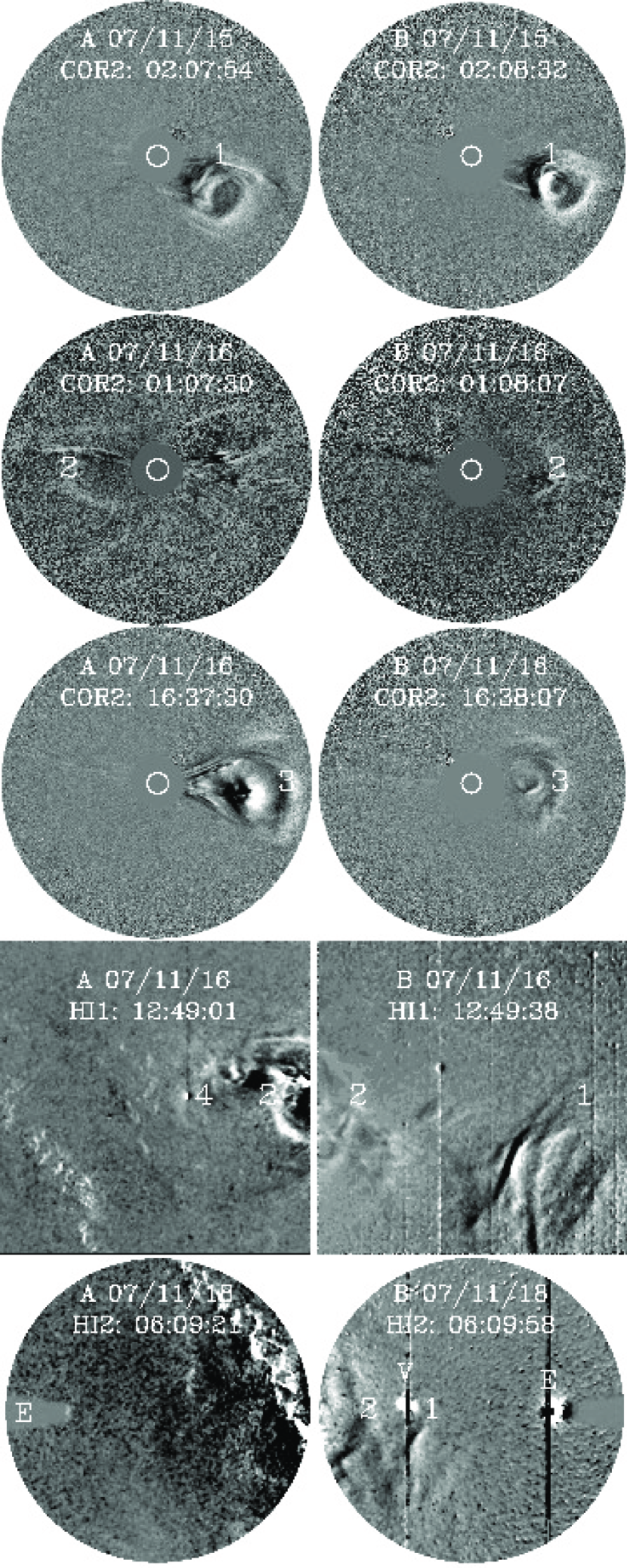
Figure 2: Running difference images of the 2007 November CMEs observed by STEREO A (left) and B (right) near simultaneously. The top three rows display COR2 images of the three CMEs, respectively, and the bottom two rows show images from HI1 and HI2. The numbers, corresponding to the tracks in Figure 3, mark the locations (obtained from Figure 3) of the features. The positions of the Earth and Venus are labeled as E and V. The Earth is in the trapezoidal zone of STEREO A (the Earth occulter). (Animations of this figure are available in the online journal.)

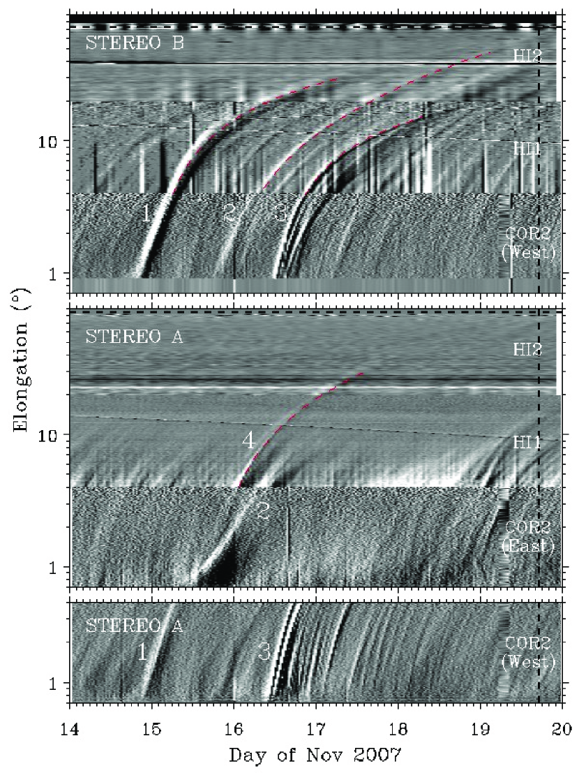
Figure 3: Time-elongation maps constructed from running difference images of COR2, HI1 and HI2 along the ecliptic plane for STEREO A and B. Data from the western part of COR2 (90^∘ clockwise from the ecliptic north) are also shown for STEREO A, as required by the triangulation analysis for CMEs propagating west of the two spacecraft (see Figure 1). The numbers indicate four tracks associated with the CMEs. The red curves show the fits to the tracks in HI1 and HI2. The vertical dashed line indicates the arrival time of a CME-driven shock at the Earth, and the horizontal dashed line marks the elongation angle of the Earth.

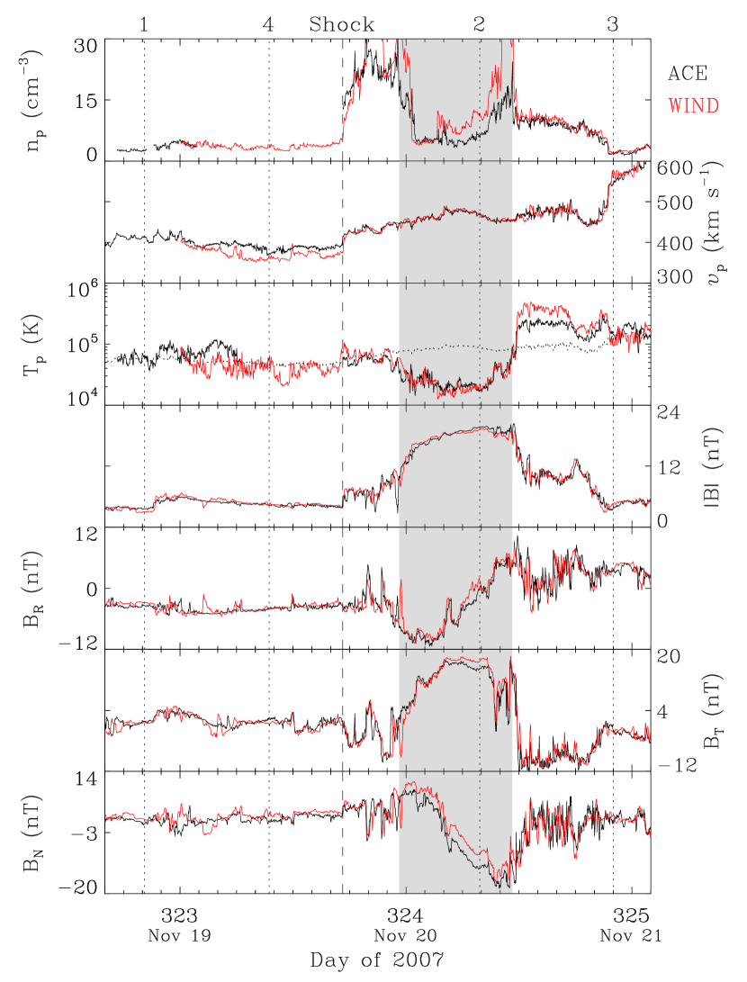
Figure 5: Solar wind plasma and magnetic field parameters across the MC observed by ACE (black) and WIND (red). From top to bottom, the panels show the proton density, bulk speed, proton temperature, and magnetic field strength and components. The shaded region indicates the MC interval. The MC-driven shock and the predicted arrival times of the four features at 1 AU are marked by the vertical dashed and dotted lines, respectively. The dotted curve in the third panel denotes the expected proton temperature from the observed speed.

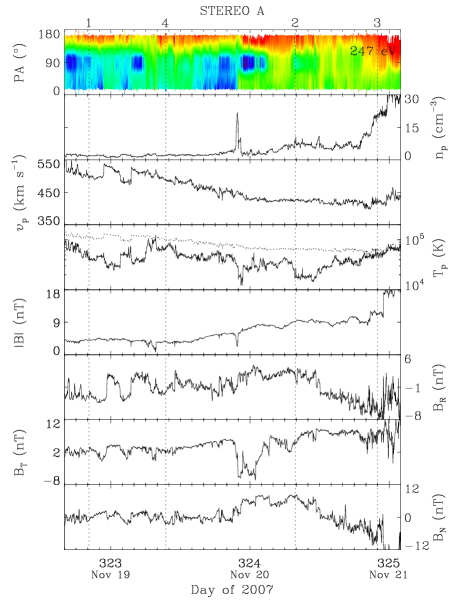
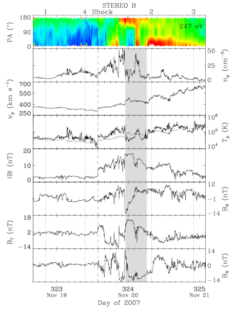
Figure 6: Similar format to Figure 5, but for the measurements at STEREO A (left) and B (right). Also shown is the pitch-angle (PA) distribution of 247 eV electrons (top). The color shading indicates the values of the electron flux (descending from red to blue).

Three consecutive CMEs are observed on 2007 November 14-16 when STEREO A and B are separated by $\gamma\simeq 40^{\circ}$. During this time, $d_{A}\simeq 0.97$ AU, and $d_{B}\simeq 1.04$ AU. Figure 2 shows two synoptic views of the events from the two spacecraft. The first and third events, which occur on November 14 and 16 respectively, appear at the west limb of the Sun for both STEREO A and B, so the scenario shown in the right panel of Figure 1 will apply. Apparently, these two CMEs show different elongation angles for the two spacecraft, which can be converted to propagation direction and radial distance using the geometric triangulation method. Neither of these two events is observed by the HI instruments on STEREO A since their FOVs are off to the east. The second CME, which occurs on November 15, is observed by both STEREO A and B but at opposite sides of the Sun, so it is likely an Earth-directed event. For STEREO B, the first and second CMEs can even be seen in HI2 whereas the third one is only faintly visible in HI1 (see Figure 3 and animations online). The first CME quickly becomes flattened and distorted into a concave-outward shape, presumably owing to the interaction with ambient structures and/or solar wind speed gradient (Liu et al., 2006a, 2008a, 2009b; Savani et al., 2010). A wave-like structure is observed ahead of the second CME, best seen in HI1 of STEREO A, which may be ambient structures deflected by the CME-driven shock or the shock itself. In situ measurements at 1 AU do show a shock preceding the ejecta (see Figures 5 and 6). Animations made of composite images (with FOVs to scale) are available online, which show the evolution of the CMEs (and the shock) in virtually the entire Sun-Earth space.

Note that the HI images require a special processing procedure prior to the running differencing. This is necessary due to the large FOVs and increasing faintness of CME signals as they move further from the Sun. A background, computed from several days worth of data before the events, is first subtracted from each image to remove the F corona. We then align adjacent images before making the running-difference sequence in an effort to eliminate the stellar background. Finally, a median filter is applied to the running-difference images to reduce the residual stellar effects. Artifacts are still visible in Figure 2 (bottom two rows), including the diffuse Milky Way galaxy in STEREO A and vertical streaks in STEREO B (resulting from saturation due to planets).

A radial slit with a width of 64 pixels around the ecliptic plane is extracted from the difference images of COR2, HI1 and HI2. Resistant means of the running difference intensities, taken over the 64 pixels, are then stacked as a function of time and elongation, which results in the time-elongation maps shown in Figure 3. The elongation angles are plotted in a logarithmic scale to expand COR2 data. Tracks associated with the three CMEs and the shock can be identified from the maps: the elongation angles along the tracks are marked in the difference images to seek the corresponding structures (see Figure 2). The shock driven by the second CME gives rise to the fourth track as indicated in the maps of STEREO A; the remaining three tracks are produced by the edges (mostly leading edges) of the CMEs in the ecliptic plane. A smooth transition is observed in the tracks from COR2 to HI1 and then from HI1 to HI2, indicative of a continuous tracking of the same event over large distances. Also shown is the elongation angle of the Earth, which is about $84^{\circ}$ for STEREO A and $72^{\circ}$ for STEREO B.

Elongation angles of the CMEs (and the shock as well) can then be extracted from the tracks, usually along the trailing edge of the tracks (the black/white boundary) where the contrast is the sharpest. When geometric triangulation is feasible with data from both spacecraft, interpolation is performed to get elongation angles at the same time tags for STEREO A and B as required by the triangulation analysis; the values of the elongation angles are then input to an appropriate set of equations to calculate the propagation direction and radial distance (see §2.3). When data are available from only one spacecraft, we fit the elongation angles using equation (5) assuming a constant propagation direction and speed. Only HI1 and HI2 data are used in the track fitting. Table 1 lists the propagation direction, speed and predicted arrival time at 1 AU obtained from the track fitting. The propagation direction ($\beta_{A}$ or $\beta_{B}$) is converted to an angle with respect to the Sun-Earth line. If the angle is positive (negative), the CME feature would be propagating west (east) of the Sun-Earth line in the ecliptic plane. The fits are also plotted in Figure 3 over the time-elongation maps; a good agreement with the tracks is achieved.

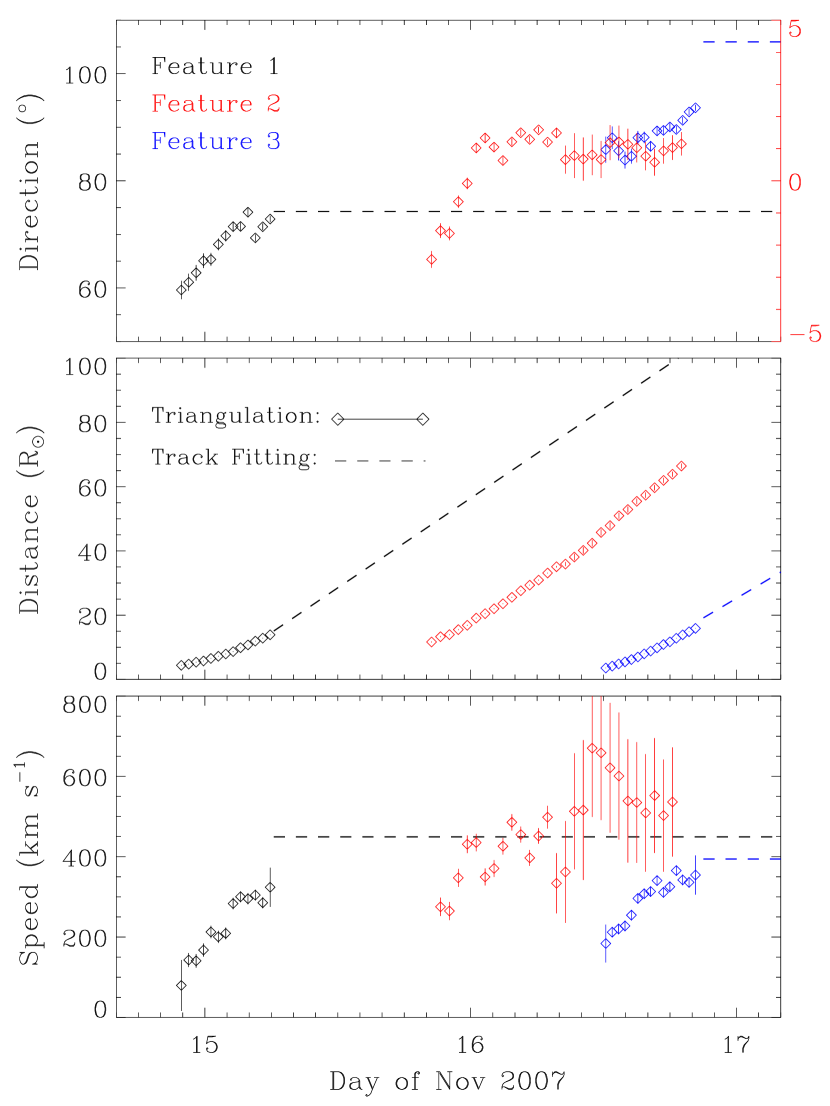
Figure 4: Propagation direction, radial distance and speed of features 1 (black), 2 (red) and 3 (blue) derived from geometric triangulation (scatter) and track fitting (dashed lines). For feature 2, the propagation direction is scaled by the right axis (red). Track fitting results for feature 2 are not plotted here (but see Table 1). The speeds (scatter) are calculated from adjacent distances using a numerical differentiation with three-point Lagrangian interpolation. Error bars represent uncertainties mathematically derived from the measurements of elongation angles.

Figure 4 shows the CME kinematics resulting from the triangulation analysis and the comparison with track fitting. An uncertainty of 10 pixels, which is roughly 0.04^∘, 0.2^∘ and 0.7^∘ for COR2, HI1 and HI2 respectively, is applied to the measurements of elongation angles. This uncertainty does not necessarily reflect the errors due to the effects of projection, Thomson scattering and CME geometry, but is mainly to show the sensitivity of the technique to the errors in the elongation angle measurements (see Appendix A for error analysis). Note that the diagram shown in the right panel of Figure 1 is invoked for the first and third CMEs while the one shown on the left is used for the second event. For the first and third CMEs, triangulation is applied only to COR2 data; neither of the two events is observed by the HIs of STEREO A since their FOVs are off to the east side of the Sun. The second CME is not visible in HI2 of STEREO A (see Figures 2 and 3), so triangulation can only be performed out to HI1. The first CME has a propagation direction increasing from about 60^∘ to 73^∘ west of the Sun-Earth line, comparable to the estimate from track fitting; the radial distances connect well with the fit ones, except that the fit speed is larger than that estimated from geometric triangulation. Agreement between triangulation and fitting is also seen for the third CME in terms of distance and speed, but the propagation angle from track fitting seems larger, 106^∘ compared with 93^∘. The largest difference between triangulation and fitting is observed for the second CME, with 1^∘ versus $17^{\circ}$ for the propagation direction and 500 km s^-1 versus 390 km s^-1 for the speed (see Table 1).

The third CME is about $20^{\circ}$ west of the first one as determined from geometric triangulation, which is almost the same angle the Sun has rotated to the west during the time between the launch of the two events. Therefore, these two CMEs are likely to originate from the same source region on the Sun. The same conclusion has been reached by Howard & Tappin (2008) in their geometrical analysis of the two limb events. Only the second CME can be tracked out to HI1 by the triangulation technique. Its propagation direction changes from eastward to westward rapidly and then stays roughly constant at $1^{\circ}$ west of the Sun-Earth line. This transition is likely true: at the early stage STEREO A observed an elongation larger than STEREO B (see the second row of Figure 2), but later the elongations seen by the two spacecraft are similar (see the fourth row of Figure 2). The speed of the second CME first increases and then decreases into the FOV of HI1, which indicates a strong interaction of the CME with the background heliosphere when not far from the Sun. Also note that all the three CMEs (and the 2008 December 12 CME as well) undergo a westward migration at the beginning. We suspect that this is a universal feature for all CMEs: the strong magnetic field within CMEs, which is still connected to the Sun as CMEs move outward, would produce a tendency for the ejecta to co-rotate with the Sun (see discussion in §4.1).

The association with in situ signatures can now be established. Figure 5 shows an MC identified from near-Earth solar wind data based on the depressed proton temperature, strong magnetic field and smooth rotation of the field. The magnetic field is measured in RTN coordinates (in which R points from the Sun to the spacecraft, T is parallel to the solar equatorial plane and points to the planet motion direction, and N completes the right-handed triad). A similar plasma and magnetic field structure is observed at ACE and WIND. A preceding shock, as can be seen from simultaneous increases in the plasma density, bulk speed, temperature and magnetic field strength, passed the spacecraft at 17:17 UT on November 19. The density within the MC is comparable to that of the ambient solar wind (upstream of the shock) but much smaller than in the sheath (a transition layer between the MC front and the shock) and trailing region. Also plotted are the predicted arrival times of the four features estimated from track fitting (see Table 1). The first CME is far earlier than the actual arrival while the third one is much later; their propagation directions also seem too westward to reach the Earth. Only the second CME shows the right propagation direction and arrival time at 1 AU. Therefore, it must be the second CME that is responsible for the MC. The predicted shock arrival time is about 8 hr earlier than observed at the Earth.

The conclusion about the association is further supported by in situ data from STEREO A and B as shown in Figure 6. Only a density spike is observed at STEREO A, which may be produced by the disturbance associated with the MC. STEREO B observed a shock at 13:48 UT on November 19 and a subsequent MC on November 20. Presumably this is the same event as observed near the Earth. The MC interval is mainly determined from the strong magnetic field and rotation of the field. Irregularities in the magnetic field are seen within the MC, indicative of distortion by ambient structures. Enhanced suprathermal electrons are observed during the time period but mainly in a direction either parallel or anti-parallel to the magnetic field (i.e., no bi-directional streaming). Again, only the second CME shows the correct arrival time. The shock arrives at STEREO B about 4 hr later than predicted by track fitting. Note that the shock arrives at STEREO B before it arrives at the Earth although STEREO B is slightly further from the Sun than the Earth. This may indicate either a complex structure of the shock or a change in the propagation direction owing to interactions with the ambient medium. It is worth mentioning that the shock has a substantially large standoff distance from the MC (compared with the radial width of the MC which is about 0.08 AU); this seems consistent with imaging observations from HI1 of STEREO A (see Figure 2 and online animations).

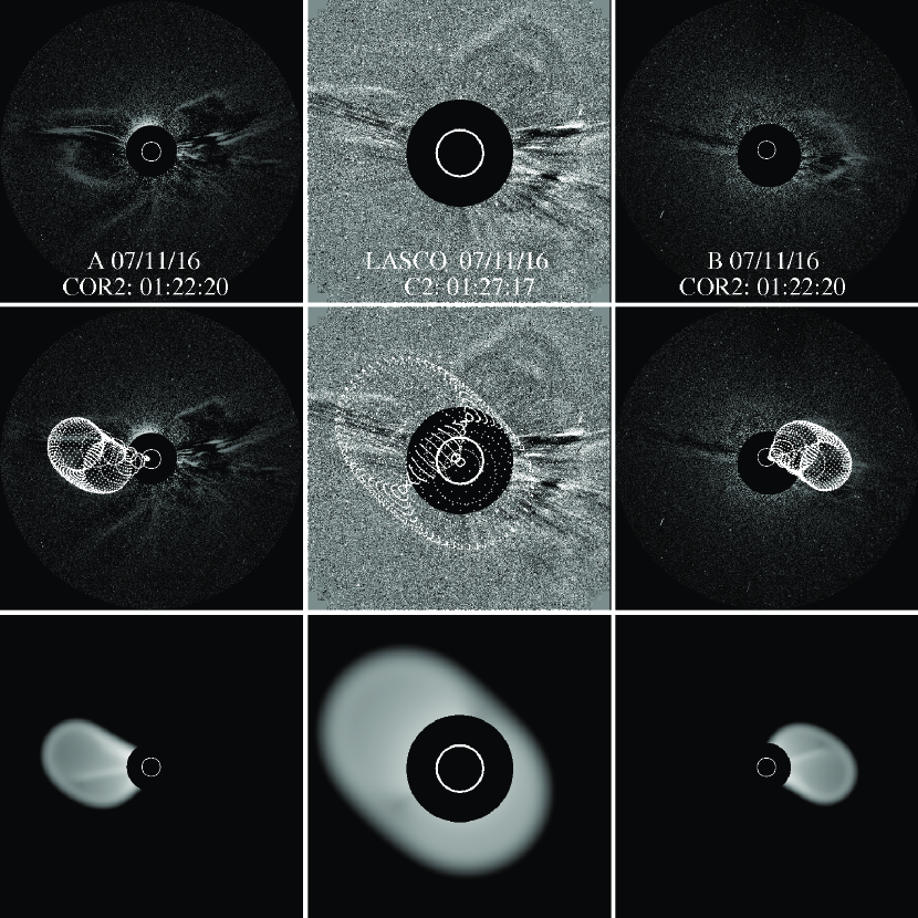
Figure 7: Observed (top) and modeled (middle and bottom) images of the second CME as viewed from three spacecraft. The middle panels show a wireframe rendering of the CME superposed on the observed image, and the bottom panels are simulated white-light images.

Now that the correspondence has been established, we can compare the structure determined from coronagraph image modeling with in situ reconstruction. Figure 7 shows the observed and modeled images of the second CME from three viewpoints. The fit is obtained by adjusting the model parameters to match STEREO A and B images; LASCO images are used to verify the fit. There are multiple structures in LASCO with the most prominent one moving toward the northwest; a very faint front on the left side, which is halo like and barely seen in the still image, fits the model well. We actually tried to fit the front on the northwest at first, but then a good match with STEREO A and B images cannot be obtained simultaneously. The fit, which is considered to match the three views, gives a propagation direction about $2^{\circ}$ east of the Sun-Earth line and $\pm 1^{\circ}$ relative to the ecliptic plane as well as a rope tilt angle about $-36^{\circ}$ (clockwise from the ecliptic; see Figure 7). Whether the propagation direction is above or below the ecliptic plane cannot be determined accurately from image modeling. The image modeling suggests that the CME is headed almost right toward the Earth, consistent with the geometric triangulation analysis. Other CMEs are also simulated by the forward modeling technique. Table 2 shows the resulting propagation direction and rope orientation. The propagation angle of the 2007 November 14 CME relative to the Sun-Earth line determined from image modeling is similar to the estimate from geometric triangulation; for the 2007 November 16 CME, image modeling gives a larger angle but the difference is not significant (123^∘ versus 93^∘).

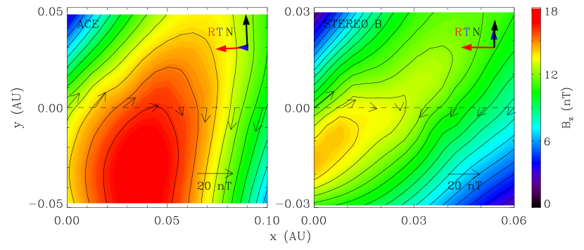
Figure 8: Reconstructed cross sections of the MC at ACE (left) and STEREO B (right). Black contours show the distribution of the vector potential, and the color shading indicates the value of the axial magnetic field. The dashed line marks the trajectory of each spacecraft (which can be used as a proxy for the ecliptic plane projected on the cross section). The thin black arrows denote the direction and magnitude of the observed magnetic fields projected onto the cross section, and the thick colored arrows show the projected RTN directions.

Figure 8 displays the cross sections of the MC reconstructed from the in situ data at ACE and STEREO B, respectively. The contours represent nested helical magnetic field lines projected onto the cross section in a flux-rope frame (with $x$ almost along the spacecraft trajectory and $z$ in the direction of the axial field). Table 3 gives the times, estimated axis orientations and magnetic field chiralities for the MCs of interest. The field configuration is left-handed at both ACE and STEREO B, as can be seen from the transverse fields along the spacecraft trajectory. The in situ reconstruction gives an axis elevation angle of about $-1.4^{\circ}$ in RTN coordinates at ACE while $-33.8^{\circ}$ at STEREO B. The flux-rope tilt angle at STEREO B is comparable to the estimate from image modeling ($-36^{\circ}$), but near the Earth it becomes significantly smaller. The axis azimuthal angle is $106.7^{\circ}$ at ACE and $91.8^{\circ}$ at STEREO B (RTN), so the flux-rope axis is nearly perpendicular to the radial direction (R), which seems consistent with the scenario shown in Figure 7 (see the simulated image for LASCO). The RTN directions are projected onto the cross section in order to compare reconstruction results with observations. For example, as ACE moves along $x$ in the flux-rope frame, it would see a $B_{R}$ component that is first negative and then positive, a $B_{T}$ that is largely positive (since the flux-rope axis is almost along T), and a $B_{N}$ that is first positive and then negative (see the field orientation along the spacecraft trajectory). A similar magnetic field structure is observed at STEREO B, but note a larger axis elevation angle than at ACE. These results are consistent with the in situ measurements (see Figures 5 and 6).

The reconstructed cross sections at both ACE and STEREO B show a maximum axial field below the ecliptic plane (as shown by the spacecraft trajectory). The overall propagation direction of the CME at 1 AU is thus likely to be southward. This can be easily understood from the reconstruction results at ACE: the flux rope axis is nearly parallel to the ecliptic plane and perpendicular to the radial direction, and ACE crosses the MC above the flux-rope axis, so the flux rope should be largely below the ecliptic plane. The interpretation about the propagation direction is consistent with the reconstruction at STEREO B although the flux rope is more tilted there. Coronagraph image modeling of the CME indicates a propagation direction within $\pm 1^{\circ}$ of the ecliptic plane. The propagation direction as well as the flux-rope orientation may change during the transit from the Sun to 1 AU, possibly owing to interactions with the background heliosphere (also see Liu et al., 2008b).

The Earth-directed event shows a few interesting while puzzling features that deserve a further study. The CME is clearly visible in HI2 of STEREO B but hardly discernible in HI2 of STEREO A (see Figures 2 and 3), which indicates a propagation direction closer to STEREO A than B (i.e., west of the Sun-Earth line). Howard & Tappin (2009) obtain a central longitude of about $-17^{\circ}$ (i.e., almost directly toward STEREO B) by fitting the CME as a spherical shell. Our track fitting, geometric triangulation and image forward modeling give a propagation angle of $17^{\circ}$, $1^{\circ}$ and $-2^{\circ}$ (note the signs), respectively. The estimate of the CME propagation direction by Howard & Tappin (2009) seems to contradict with the HI observations but appears more or less consistent with the in situ measurements, i.e., the ICME impacts the Earth and STEREO B but only grazes STEREO A (see Figures 5 and 6). Note that a more regular flux-rope structure is observed at the Earth than at STEREO B. As mentioned earlier, the shock arrives at STEREO B before it arrives at the Earth although STEREO B is 0.04 AU further from the Sun. A high-speed flow is observed following the ICME (see Figures 5 and 6), which may squeeze the ejecta from behind. All these features indicate a complex structure (other than spherical) and propagation direction of the event due to interactions with the ambient flows.

3.2 2008 December 12-17 Event

The kinematics of the 2008 December 12 CME have been studied in paper 1 with the geometric triangulation method. Here we briefly summarize some of the results relevant to the present work. During the time of the CME, the longitudinal separation between STEREO A and B is about $\gamma\simeq 86.3^{\circ}$, and the distances of the two spacecraft from the Sun are $d_{A}\simeq 0.97$ AU and $d_{B}\simeq 1.04$ AU. The CME is associated with a prominence eruption in the northern hemisphere. It produces two tracks in the time-elongation maps, one corresponding to the leading edge of the CME and the other the trailing edge, which extend out to 50^∘ elongation for both STEREO A and B. The triangulation analysis assuming $d_{A}=d_{B}=1$ AU in paper 1 gives propagation directions generally within $10^{\circ}$ of the Sun-Earth line, radial distances out to 150 solar radii or 0.7 AU, and predicted arrival times and radial speeds consistent with the near-Earth in situ measurements around an MC. Note that the CME also shows a westward migration when it is within about 20 solar radii from the Sun. Refer to paper 1 for details and animations of the imaging observations.

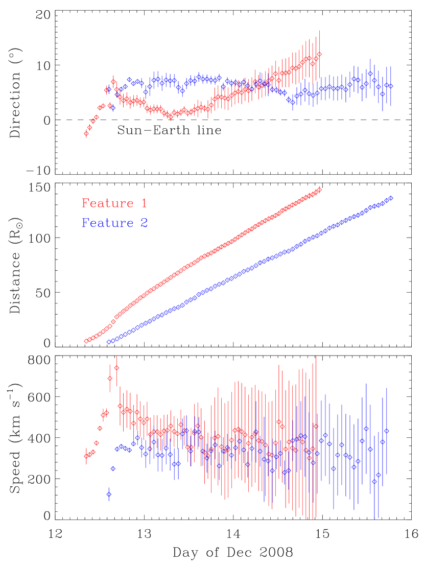
Figure 9: Propagation angle, radial distance and speed of the leading (red) and trailing (blue) edges of the 2008 December 12 CME derived from geometric triangulation analysis. Similar format to Figure 4.

We repeat the analysis of paper 1 using the exact values of the spacecraft distances and plot the results in Figure 9. Differences are observed in the trends of the propagation angle but only at large distances. The CME leading edge shows a continuous westward deflection in the FOV of HI2, rather than suddenly turns to the east of the Sun-Earth line as indicated in paper 1. The CME trailing edge has a generally constant propagation angle with respect to the Sun-Earth line in both HI1 and HI2, i.e., no turn to the east of the Sun-Earth line. Other results, such as the radial distance and speed, are almost the same as in paper 1 and consistent with the in situ measurements around the MC. With the association between solar observations and in situ signatures established by the triangulation analysis, we can now compare the structures and propagation directions determined from coronagraph image modeling and in situ reconstruction.

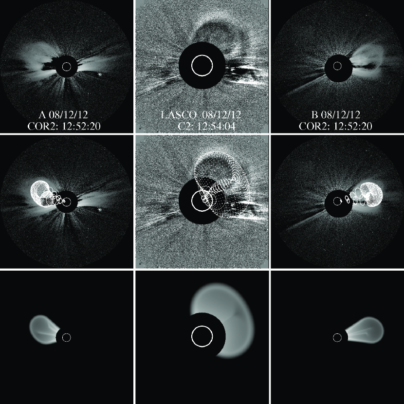
Figure 10: Similar format to Figure 7, but for the 2008 December 12 CME.

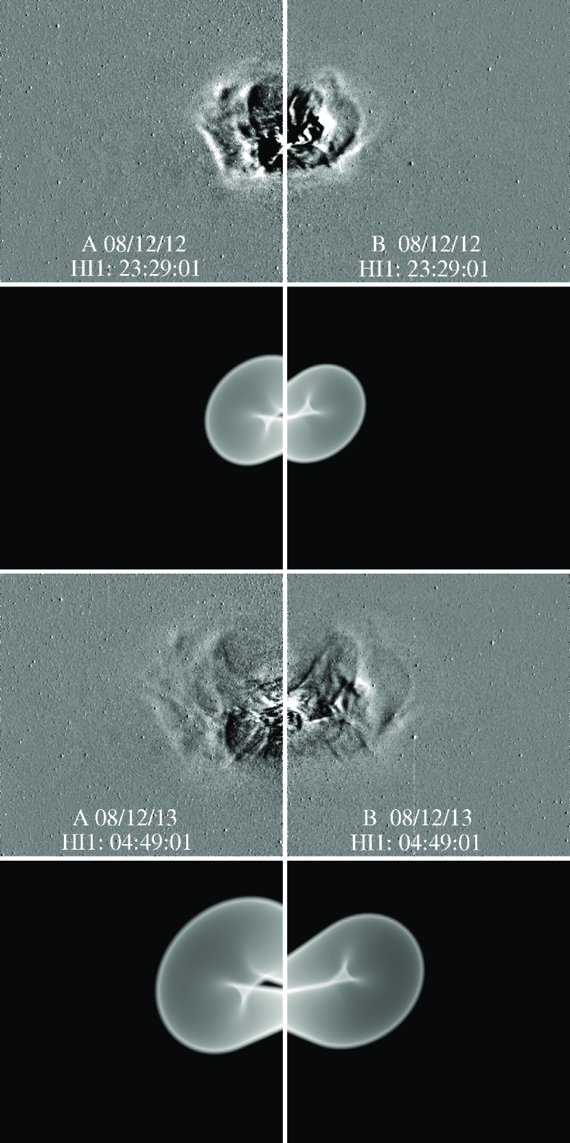
Figure 11: Comparison between HI1 observations and corresponding simulations for the 2008 December 12 CME. Views from STEREO A (left) and B (right) at two times are shown by the top and bottom panels, respectively.

Figure 10 shows the comparison between observed and modeled coronagraph images of the 2008 December 12 CME from three viewpoints. All the three views are reproduced fairly well; the spatial extent of the simulated CME also agrees with the observations, as shown by the wireframe rendering superposed on the observed image. The fit from the forward modeling gives a propagation direction about 10^∘ west of the Sun-Earth line and 8^∘ above the ecliptic plane, and a flux-rope tilt angle about $-53^{\circ}$ clockwise from the ecliptic plane (see Table 2). The propagation angle relative to the Sun-Earth line determined from image modeling is consistent with the estimate from the geometric triangulation analysis. The basic structure of the CME is not significantly distorted out to the FOV of HI1 (close to the Sunward edge), as can seen in Figure 11; it is remarkable that at large distances the CME can still be simulated by such a rope-like model.

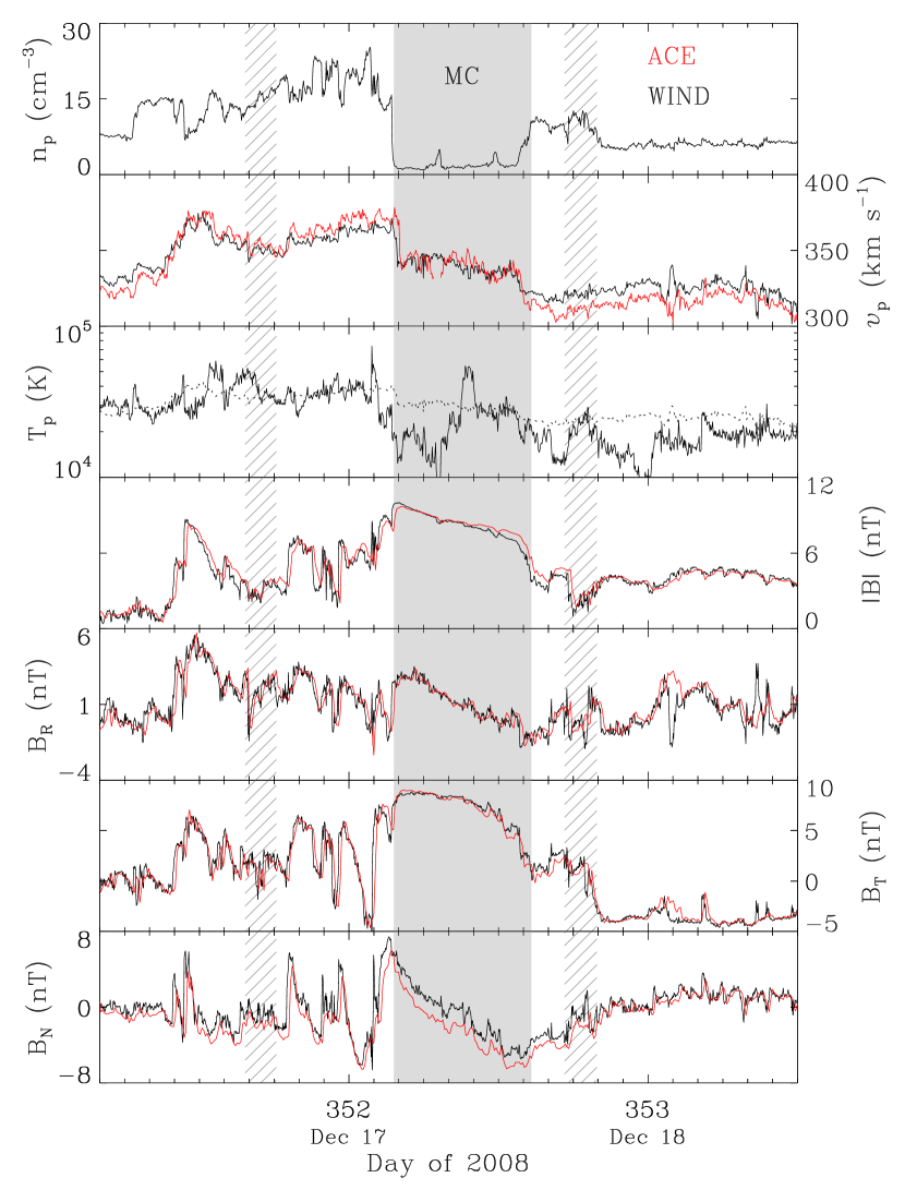
Figure 12: Similar format to Figure 5, but for the measurements of the 2008 December 17 MC at WIND (black) and ACE (red). The hatched area shows the arrival times (with uncertainties) of the CME leading and trailing edges predicted by the geometric triangulation technique.

Figure 12 shows the corresponding MC near the Earth identified from the strong magnetic field and smooth rotation of the field. Again, ACE and WIND observed a similar velocity and magnetic field structure, but ACE does not have valid measurements of the proton density and temperature due to the low solar wind speed. The predicted arrival times of the CME leading and trailing edges are good to within a few hours. Note that what is being tracked is enhanced density regions outside the flux rope; the CME front has swept up and merged with the ambient solar wind during its propagation in the heliosphere. The density within the flux rope is lower than that of the ambient solar wind owing to expansion, so the flux rope probably cannot be imaged in white light at large distances (especially in the FOV of HI2). Two small density spikes are observed within the MC, reminiscent of the prominence material. No ICME signatures are observed at STEREO A. STEREO B observed a depressed proton temperature between 14:00 UT on December 16 and 02:00 UT on December 17, but at the same time the magnetic field is not enhanced and does not show a coherent rotation. It is likely that the ICME missed the two spacecraft given such a small event and large spacecraft separation in longitude (or the ICME may have been so well assimilated into the ambient structures that it is no longer recognizable).

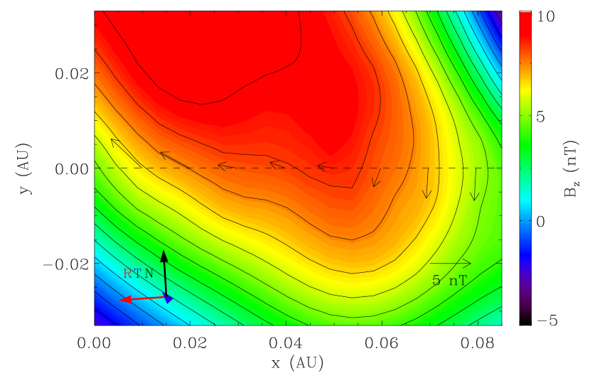
Figure 13: Cross section of the 2008 December 17 MC reconstructed from WIND measurements. Similar format to Figure 8.

The MC cross section reconstructed from WIND data is displayed in Figure 13. The transverse magnetic fields along the spacecraft trajectory indicate a left-handed flux-rope configuration. The in situ reconstruction gives a flux-rope tilt angle about $-6.4^{\circ}$ and azimuthal angle about $94.9^{\circ}$ in RTN coordinates (see Table 3). The flux-rope tilt angle is much smaller than the estimate from image modeling ($-53^{\circ}$). The reconstructed cross section shows a maximum axial field above the ecliptic plane (as shown by the trajectory of WIND), so the overall propagation direction of the CME at 1 AU is likely northward. This is consistent with the results from image forward modeling. Again, the RTN directions are projected onto the cross section in order to compare reconstruction results with in situ measurements. As shown by the field orientation along the spacecraft trajectory, the magnetic field would have a $B_{R}$ component that is first positive and then slightly negative, a $B_{T}$ that is largely positive (since the flux-rope axis is almost along T), and a $B_{N}$ that is first positive and then negative. This is exactly observed at WIND and ACE (see Figure 12).

Davis et al. (2009) perform the same track fitting approach on the HI observations of the event as in §3.1 and obtain similar results (including propagation direction, speed and arrival time at 1 AU). Refer to paper 1 for a comparison between the geometric triangulation and track fitting for this event. Lugaz et al. (2010) study the same event using only HI data with a similar triangulation technique but assume the CME as a spherical front attached to the Sun (see Appendix B). Their analysis yields a similar but somewhat larger propagation angle. It should be noted that, although Lugaz et al. (2010) argue their approach may be more appropriate than our triangulation technique, they did not provide any comparison with in situ measurements, which is the best means to test the results (e.g., predicted arrival time and speed at 1 AU). Also see Appendix B for a discussion of their method.

4 Conclusions and Discussion

We constrain the global structure and kinematics of CMEs by combining image observations with in situ measurements. The global structure of CMEs is reproduced from coronagraph observations by a forward modeling technique, while the in situ counterpart at 1 AU is reconstructed with the GS method. Propagation of CMEs between the Sun and 1 AU is studied with a geometric triangulation technique, which enables a proper association between imaging and in situ observations.

In addition to the case studies described in §3, we are also performing a statistical analysis of Earth-directed events with joint imaging and in situ observations. All the results, including movies made of composite images, time-elongation maps, CME kinematics derived from triangulation analysis, plots showing in situ signatures and comparison with triangulation analysis, and in situ reconstruction if possible, are compiled into our catalog of STEREO Earth-directed CMEs at http://sprg.ssl.berkeley.edu/~liuxying/CME_catalog.htm. One focus of the statistical study is on the evaluation of the geometric triangulation technique. Our preliminary results from the statistical study show that the CME arrival time and speed at the Earth are generally well predicted by the triangulation method. All the CMEs studied so far exhibit more or less a westward motion at their acceleration phase, similar to the 2007 November and 2008 December events. Below we will summarize and discuss the results mainly based on the case studies described in §3.

4.1 Consistency and Caveats

Imaging observations and in situ measurements are two basic means in probing CME properties. They are essentially distinct in terms of the physics relied on to do the measurements. The following findings from this work may help pave the way to link imaging and in situ observations, as required by the proper treatment of the CME problem and practical space weather forecasting.

First, CME propagation directions derived from different methods are generally consistent with each other. For the 2007 November 15 and 2008 December 12 CMEs, both the geometric triangulation analysis and coronagraph image modeling result in propagation directions almost right toward the Earth; in situ measurements near the Earth show corresponding signatures with the correct timing. A rough agreement between triangulation analysis and image modeling is also obtained for the 2007 November 14 and 16 events which propagate west of STEREO A and B; the possibility for them to reach the Earth is excluded based on the timing and their propagation directions. In situ reconstruction of the 2008 December 12 event at 1 AU shows a maximum axial magnetic field above the ecliptic plane, which agrees with the overall northward propagation obtained from coronagraph image modeling. For the 2007 November 15 CME, in situ reconstruction at 1 AU indicates a southward propagation, but a rigorous comparison with coronagraph image modeling is not possible.

Second, the geometric triangulation technique shows a promising capability to link solar observations with corresponding in situ signatures at 1 AU and to predict CME arrival at the Earth. Association between solar observations and in situ signatures at 1 AU is often ambiguous due to the large distance gap; the situation becomes worse for consecutive CMEs like the 2007 November events. This may be the main reason that most CME studies are focused only on the Sun or ICME signatures near the Earth. The geometric triangulation technique, which can determine both propagation direction and radial distance continuously over an extensive region of the heliosphere and thus arrival time at 1 AU, provides a means to identify the unique association between solar observations and in situ signatures. It should be stressed that, even though the effect of CME geometry is not taken into account, the technique still presents a reasonable accuracy in determining CME kinematics and arrival time as shown by the comparison with in situ measurements and coronagraph image modeling.

Third, the flux rope within CMEs probably cannot be imaged at large distances by the HIs due to expansion. The tracks that extend to large elongations in time-elongation maps are usually CME edges, so what is being tracked is enhanced density regions outside the flux rope. This finding is confirmed by in situ measurements. On average, the plasma density within the flux rope at 1 AU is comparable to the ambient density, i.e., about 5 cm^-3 (see Liu et al., 2006b, c, and Figures 5, 6 and 12). A correlation study of solar wind stream interaction regions between HI2 images and in situ measurements at 1 AU seems to suggest a density threshold of about 15 cm^-3 at 1 AU for HI2 observations (Sheeley et al., 2008). Therefore, the density within the flux rope is usually far below the HI2 sensitivity. This raises a serious problem for space weather forecasting: the arrival time of the flux rope, which has the most hazardous southward magnetic field, cannot be predicted precisely from imaging observations. The uncertainty could be as large as 10 hr depending on the size of the sheath region; the average duration of the sheath at 1 AU is about 14 hr when the ejecta is preceded by a shock (Liu et al., 2006c). However, it is usually the shock that brings the sudden commencement of geomagnetic storms; the sheath region is also geoeffective although the magnetic field is turbulent there (Liu et al., 2008a).

Fourth, the flux-rope orientation derived from in situ reconstruction at 1 AU may have a large deviation from that determined by coronagraph image modeling. The image modeling of the 2007 November 15 CME gives a tilt angle of about $-36^{\circ}$, much larger than the estimate from in situ reconstruction near the Earth ($-1.4^{\circ}$), although a similar result is obtain from the in situ data at STEREO B. For the 2008 December 12 CME, image modeling and in situ reconstruction yield a flux-rope tilt angle about $-53^{\circ}$ and $-6.4^{\circ}$ respectively, an even larger discrepancy. These results seem contrary to the suggestion of Rouillard et al. (2009), which is based on a single case study, that the flux-rope orientation can be predicted from white-light images. The lack of consistency with in situ measurements is likely accounted for by the evolution of the flux rope in interplanetary space, e.g., distortion/deflection by the ambient structures and/or flux rope rotation between the Sun and 1 AU. As indicated by in situ measurements, the density structures that appear to be part of a CME in imaging observations are actually different regions from the flux rope. The envelope fit by the image forward modeling might not reflect precisely the exact size and location of the flux rope in coronagraph observations. Faraday rotation measurements of the CME magnetic field using polarized radio signals (Liu et al., 2007) are thus extremely valuable given the limited capability of imaging observations in determining the magnetic field orientation.

Fifth, the triangulation analysis indicates that all the CMEs studied here undergo a westward migration with respect to the Sun-Earth line at their early stage. The 2007 November 14, 2007 November 15 and 2008 December 12 CMEs move westward by about $13^{\circ}$, $4^{\circ}$ and $10^{\circ}$, respectively; the 2007 November 16 event does not achieve a radial motion in the FOV of COR2 even after it has moved to the west by $8^{\circ}$. These rotation angles should be considered as the lower limits since COR1 observations are not taken into account. The westward motion occurs mainly when CMEs are accelerated (see Figures 4 and 9). Other events in our CME catalog also show more or less a westward motion at their acceleration phase. If this were an effect of CME geometry, then there would be no systematic westward motion, i.e., the change in the propagation angle would be randomly distributed between eastward and westward, which is apparently not the case. Also note that, with the two views, the propagation angle and distance are linearly independent (see equation 4). To the best of our knowledge, this is the first time that a systematic westward migration of CMEs relative to the Sun-Earth line is discovered at the acceleration phase. A direct consequence of the westward transition is that all techniques for tracking CMEs, which assume a radial propagation from the solar source region, may lead to a considerable error in the propagation direction. Due to this westward transition, CMEs that occur at the eastern hemisphere of the Sun would have a greater potential to reach the Earth than events from the western hemisphere.

The westward motion, which is expected to be a universal feature for CMEs at the early stage, can be explained by the magnetic field connecting the Sun and CMEs. As the magnetic field is frozen in the CME plasma, the Sun and a CME would be coupled together by the magnetic field out to a distance, the so-called Alfvén radius $r_{A}$, within which the flow energy is dominated by the magnetic field energy, i.e., $\rho v^{2}/2\leq B^{2}/2\mu_{0}$. Here $\rho$, $v$ and $B$ are the mass density, speed and magnetic field strength of the CME. Therefore, the magnetic field inside CMEs produces a tendency toward co-rotation with the Sun. More specifically, the westward migration of CMEs with respect to the Sun-Earth line is caused by the rotation of the Sun when the motion of CMEs is controlled by the magnetic field. The value of $r_{A}$ or co-rotation angle is determined by the interplay between the density, magnetic field and acceleration of CMEs. The CMEs examined here show an Alfvén radius of 10-20 solar radii (the distance at which CMEs stop moving westward). This value seems larger than the counterpart of the solar wind, which is usually below 10 solar radii but depends on the solar wind source location, e.g., streamer belt, coronal holes and active regions. The westward motion of CMEs at the early stage will be further investigated in a separate paper.

4.2 Concept for Future Missions

This merged imaging and in situ study demonstrates the exciting possibility to predict CME interplanetary properties with observations from multiple vantage points. In particular, the geometric triangulation concept based on wide-angle imaging observations from STEREO can track CMEs (both propagation direction and radial distance) continuously from the Sun all the way out to the Earth. The same concept can be applied to future missions at the fourth and fifth Lagrangian points (L4 and L5), which are well situated for this purpose.

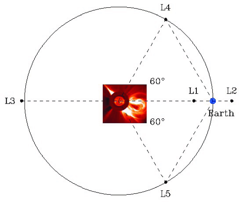
Figure 14: The five Lagrangian points of the Sun-Earth system in the ecliptic plane (not to scale). The circle represents the orbit of the Earth. L4 and L5, which form the apex of two equilateral triangles, are well situated for geometric triangulation of CME observations.

Figure 14 shows the five Lagrangian points in the Sun-Earth system. These are fixed positions in an orbital configuration where a small object (such as a spacecraft) can be theoretically stationary. L4 and L5 have the same orbit as the Earth but lie at $60^{\circ}$ ahead of and behind the Earth, respectively. Unlike STEREO A and B, they are fixed in space with respect to the Sun and Earth rather than drift away from each other. The longitudinal separation ($120^{\circ}$) between these two points is appropriate for the observation of CMEs, even wide ones. Another advantage of L4 and L5 is that they are resistant to gravitational perturbations, so they are truly stable. (L1, L2 and L3 are only meta stable; a spacecraft at these points has to use frequent propulsions to remain on the same orbit.) It would be of great merit to have dedicated spacecraft making routine observations at both L4 and L5. They are located well away from the Sun-Earth line, thus advantageous for observing Earth-directed CMEs; triangulation with two such spacecraft makes it possible to unambiguously derive the true path and velocity of CMEs; we would also be able to determine the global structure and how the Earth cuts through the structure. A hypothesized Earth-directed CME is shown in Figure 14, illustrating the exciting possibility that the interplanetary properties of the event can be accurately determined well before it impacts the Earth. This observational concept would be extremely important for CME research and represent a major step toward practical space weather forecasting.

Appendix A Error Analysis

The triangulation technique presented in §2.3 allows an easy evaluation of errors in the propagation direction and radial distance due to uncertainties in elongation measurements. The two spacecraft make independent measurements of elongation angles, so the errors can be expressed as

$$\sigma_{\beta}=\sqrt{\left(\frac{\partial\beta_{A}}{\partial\alpha_{A}}\right)^{2}\sigma^{2}_{\alpha A}+\left(\frac{\partial\beta_{A}}{\partial\alpha_{B}}\right)^{2}\sigma^{2}_{\alpha B}},$$ (A1)

$$\sigma_{r}=\sqrt{\left(\frac{\partial r}{\partial\alpha_{A}}\right)^{2}\sigma^{2}_{\alpha A}+\left(\frac{\partial r}{\partial\alpha_{B}}\right)^{2}\sigma^{2}_{\alpha B}},$$ (A2)

for the propagation direction and radial distance, respectively, where $\sigma_{\alpha}$ represents uncertainties in the elongation measurement. For a CME propagating between the two spacecraft, equations (1) and (4a) result in

$$\frac{\partial\beta_{A}}{\partial\alpha_{A}}=2f\sin\alpha_{B}\left[\sin(\alpha_{B}+\gamma)-f\sin\alpha_{B}\right]/X,$$ (A3)

$$\frac{\partial\beta_{A}}{\partial\alpha_{B}}=2\sin\alpha_{A}\left[\sin\alpha_{A}-f\sin(\alpha_{A}+\gamma)\right]/X,$$ (A4)

$$\frac{\partial r}{\partial\alpha_{A}}=\frac{d_{A}}{\sin(\alpha_{A}+\beta_{A})}\left[\cos\alpha_{A}-\frac{Y}{X}\sin\alpha_{A}\cot(\alpha_{A}+\beta_{A})\right],$$ (A5)

$$\frac{\partial r}{\partial\alpha_{B}}=\frac{-2d_{A}\cos(\alpha_{A}+\beta_{A})\sin^{2}\alpha_{A}[\sin\alpha_{A}-f\sin(\alpha_{A}+\gamma)]}{X\sin^{2}(\alpha_{A}+\beta_{A})},$$ (A6)

where

$$Y=1-\cos(2\alpha_{A})+2f\sin\alpha_{B}\sin(2\alpha_{A}+\alpha_{B}+\gamma),$$

$$X=1+f^{2}-\cos(2\alpha_{A})-f^{2}\cos(2\alpha_{B})+4f\sin\alpha_{A}\sin\alpha_{B}\cos(\alpha_{A}+\alpha_{B}+\gamma).$$

Similarly, expressions can be obtained for CMEs propagating outside the space between the two spacecraft. Consider an uncertainty of 10 pixels in the elongation angles (corresponding to 0.04^∘, 0.2^∘ and 0.7^∘ for COR2, HI1 and HI2 respectively) for the 2008 December 12 CME which is propagating almost along the Sun-Earth line. The above equations give typical errors of $0.5^{\circ}$, $1^{\circ}$ and $3^{\circ}$ in the propagation direction and 0.07, 0.6 and 1.4 solar radii in the radial distance for COR2, HI1 and HI2 respectively (see Figure 9). Also see Figure 4 for CMEs west of the two spacecraft.

Appendix B Converting Elongation to Distance

Coronagraphs and heliospheric imagers measure the elongation angles of CMEs, not radial distances. The combined effects due to projection, Thomson scattering and CME geometry form a major challenge in determining CME kinematics. Here we summarize various approximations that have been made to convert elongation to distance and discuss their advantages and restrictions.

B.1 Point P

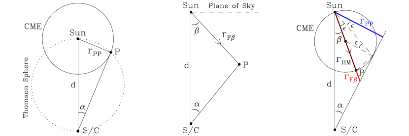
Figure 15: CME geometry assumed to convert elongation angles to radial distances. Left: Point P approximation assuming a spherical front centered at the Sun. Middle: Fixed $\beta$ approximation assuming a compact structure moving along a fixed direction. Right: Harmonic mean approximation assuming a spherical front attached to the Sun moving along a constant direction.

The point P (PP) approximation assumes a CME as a spherical front centered at the Sun (e.g., Houminer & Hewish, 1972). The brightest part of the CME to a spacecraft is the region (point P) where the CME intersects with the “Thomson surface”, a spherical front with the Sun-spacecraft line as the diameter which has the maximum Thomson scattering strength (Vourlidas & Howard, 2006), as illustrated in Figure 15 (left). The radial distance can be obtained from

$$r_{PP}=d\sin\alpha.$$ (B1)

This is the simplest way to convert elongation measurements to radial distances while taking into account Thomson scattering effects. Apparently, the CME geometry is oversimplified, and as a result the technique is only applicable to extremely wide events. Information about the propagation direction cannot be obtained. The method provides a lower limit of the distance (see below).

B.2 Fixed $\beta$

The fixed $\beta$ (F$\beta$; or fixed $\phi$ using the terminology of Kahler & Webb, 2007) approximation takes the opposite philosophy and assumes a relatively compact structure moving along a fixed radial direction, as shown in Figure 15 (middle). It is first proposed by Sheeley et al. (1999) and has been extensively used in track fitting (see §2.3). The F$\beta$ method results in

$$r_{F\beta}=\frac{d\sin\alpha}{\sin(\alpha+\beta)},$$ (B2)

which has been adopted for geometric triangulation in §2.3. The advantage of this technique is that it can provide the propagation direction (say, through track fitting). It does not take into account the effects of CME geometry and Thomson scattering, but surprisingly it achieves a reasonable accuracy in both track fitting and geometric triangulation (see §3 and paper 1). The assumption of constant propagation direction is usually not true when CMEs are close to the Sun (see §3); even far away from the Sun, they can be deflected by ambient solar wind structures. Note that, when the formula is used for geometric triangulation, the restriction to only narrow CMEs can be relaxed; the assumption of fixed radial trajectory is certainly abolished too.

B.3 Harmonic Mean

Given the restrictions of the PP and F$\beta$ approximations, a compromise would be to take the harmonic mean (HM) of these two formulas (Lugaz et al., 2009), namely,

$$\frac{1}{r_{HM}}=\frac{1}{2}\left(\frac{1}{r_{PP}}+\frac{1}{r_{F\phi}}\right),$$

which gives

$$r_{HM}=\frac{2d\sin\alpha}{1+\sin(\alpha+\beta)}.$$ (B3)

The physics behind this approximation is that CMEs are assumed as a spherical front attached to the Sun moving along a fixed radial direction; what is seen by the spacecraft is the segment tangent to the line of sight, as shown by Figure 15 (right). It can be easily proved that this CME geometry yields exactly the HM formula. Note that the angles marked as $\epsilon$ are the same. The distances of $r_{PP}$ and $r_{F\beta}$ are also indicated in the right panel of Figure 15. Apparently, the PP approximation gives the shortest distance for a given elongation angle while $r_{HM}$ (the diameter of the sphere) lies in between. Inverting equation (B3) for $\alpha$ yields

$$\alpha=\arcsin\left(\frac{r_{HM}}{\sqrt{4d^{2}-4dr_{HM}\cos\beta+r^{2}_{HM}}}\right)+\arctan\left(\frac{r_{HM}\sin\beta}{2d-r_{HM}\cos\beta}\right).$$ (B4)

A similar track fitting procedure can be applied using this new equation, but it is more complicated than equation 5, which may diminish its efficiency. The HM approximation is intended for wide CMEs only. It is argued that this technique can give better results than the PP and F$\beta$ methods (Lugaz et al., 2009). To be fair, restrictions also exist. CMEs can be significantly distorted by ambient coronal and solar wind structures (Liu et al., 2006a, 2008a, 2009b); even a uniform solar wind can easily flatten the cross section with its radial flow (Riley & Crooker, 2004; Liu et al., 2006a). Therefore, it is very difficult for CMEs to maintain a spherical shape. The assumption of a spherical front may be appropriate if the spacecraft lies in the plane of the CME loop, but in principle the flux rope can have any orientation.

B.4 Triangulation with Harmonic Mean

Motivated by the triangulation concept of Liu et al. (2010), Lugaz et al. (2010, and the present author himself) realize that the same idea can be applied with equation (B3). Figure 16 shows the diagram, which is similar to that in Figure 1 but assumes a spherical front attached to the Sun. Each spacecraft observes different plasma parcels which are assumed to be tangent to the line of sight. Equations (1) and (2) now become

$$\frac{r[1+\sin(\alpha_{A}+\beta_{A})]}{2\sin\alpha_{A}}=d_{A},$$ (B5)

$$\frac{r[1+\sin(\alpha_{B}+\beta_{B})]}{2\sin\alpha_{B}}=d_{B}.$$ (B6)

Equation (3) remains the same. This new triangulation concept might be more appropriate than the original one, if the whole flux rope lies in the ecliptic plane which is, however, not necessarily the case. As discussed above, CMEs can hardly maintain a spherical shape. Another advantage of the new method is that a CME can be seen by the HIs on both spacecraft even if its nose is outside the two spacecraft. This strength is accompanied by a dark side too. A rough knowledge of where the CME nose is with respect to the two spacecraft is needed apriori to determine which equation should be used (3a, 3b, or 3c). This is difficult due to projection effects, since the method assumes that what is observed is the region tangent to the line of sight, not necessarily the nose. Another complication is that the above equations have multiple solutions. In practice, one needs to determine which solution should be adopted. A concern is that, in some cases, the sines and cosines of the elongation and spacecraft separation angles and their combinations are such that we are not able to pick the right one.

It is immediately evident from Figure 16 why the original triangulation concept gives a reasonable accuracy even when the two spacecraft do not observe the same part of a CME: as long as the propagation direction is not very far away from the Sun-Earth line, the regions seen by the two spacecraft are not much deviated from the nose. In addition, many narrow CMEs exist, and for those events the original triangulation technique is more suitable than the new one; it works even if those CMEs are outside the space between the two spacecraft (see §3). The new triangulation notion is probably complementary to, rather than supercedes, the original concept. It would be helpful to have a statistical study with joint imaging and in situ data and comparison with realistic MHD simulations to assess the efficiency, simplicity and ease of use of these two triangulation techniques.

Table 1: Estimated parameters of the four features from track fitting

Feature	Spacecraft	Direction (∘)	Speed (km s-1)	Arrival time at 1 AU (UT)
1	STEREO B	74	449	Nov 18, 20:14
2	STEREO B	17	388	Nov 20, 07:50
3	STEREO B	106	394	Nov 20, 22:01
4	STEREO A	$-29$	474	Nov 19, 09:28

Table 2: CME parameters estimated from image modeling

Event	Time (UT)	$\theta$ (∘)	$\phi$ (∘)	$\Theta$ (∘)
2007 Nov 14 (feature 1)	Nov 15, 01:22	$-19$	61	$-18$
2007 Nov 15 (feature 2)	Nov 16, 01:22	$\pm 1$	$-2$	$-36$
2007 Nov 16 (feature 3)	Nov 16, 16:22	$-7$	123	1
2008 Dec 12	Dec 12, 12:52	8	10	$-53$

Table 3: Estimated parameters of MCs at different spacecraft

Event	Spacecraft	Shock	Start	End	$\Theta$	$\Phi$	Chirality
		(UT)	(UT)	(UT)	(∘)	(∘)
2007 Nov	ACE/WIND	Nov 19, 17:17	Nov 19, 23:17	Nov 20, 11:17	$-1.4$	106.7	L
	STEREO B	Nov 19, 13:48	Nov 19, 23:02	Nov 20, 06:14	$-33.8$	91.8	L
2008 Dec	ACE/WIND	-	Dec 17, 03:36	Dec 17, 14:38	$-6.4$	94.9	L

Figure 1: Diagrams of the geometric triangulation in the ecliptic plane for a CME feature propagating between (left), east of (middle), and west of (right) STEREO A and B. The white-light feature is denoted by the point P with its direction shown by the arrow. The dotted line indicates the orbit of the Earth, and the dashed line represents the Sun-Earth line.

Figure 16: Similar format to Figure 1, but for the geometric triangulation under the harmonic mean approximation. A spherical front attached to the Sun is assumed for the CME geometry. Only the case that the CME nose is propagating between the two spacecraft is shown. Note that, under the harmonic mean approximation, CMEs with nose outside the two spacecraft may also be seen by the HIs on both spacecraft.

References

- Billings (1966) Billings, D. E. 1966, A Guide to the Solar Corona (New York: Academic Press)
- Brueckner et al. (1995) Brueckner, G. E., et al. 1995, Sol. Phys., 162, 357
- Burlaga et al. (1981) Burlaga, L. F., Sittler, E., Mariani, F., & Schwenn, R. 1981, J. Geophys. Res., 86, 6673
- Davis et al. (2009) Davis, C. J., Davies, J. A., Lockwood, M., Rouillard, A. P., Eyles, C. J., & Harrison, R. A. 2009, Geophys. Res. Lett., 36, L08102
- Domingo et al. (1995) Domingo, V., Fleck, B., & Poland, A. I. 1995, Sol. Phys., 162, 1
- Dungey (1961) Dungey, J. W. 1961, Phys. Rev. Lett., 6, 47
- Galvin et al. (2008) Galvin, A. B., et al. 2008, Space Sci. Rev., 136, 437
- Gosling et al. (1974) Gosling, J. T., Hildner, E., MacQueen, R. M., Munro, R. H., Poland, A. I., & Ross, C. L. 1974, J. Geophys. Res., 79, 4581
- Gosling & McComas (1987) Gosling, J. T., & McComas, D. J. 1987, Geophys. Res. Lett., 14, 355
- Gosling et al. (1991) Gosling, J. T., McComas, D. J., Philips, J. L., & Bame, S. J. 1991, J. Geophys. Res., 96, 7831
- Hau & Sonnerup (1999) Hau, L.-N., & Sonnerup, B. U. Ö. 1999, J. Geophys. Res., 104, 6899
- Howard et al. (2008) Howard, R. A., et al. 2008, Space Sci. Rev., 136, 67
- Howard & Tappin (2008) Howard, T. A., & Tappin, S. J. 2008, Sol. Phys., 252, 373
- Howard & Tappin (2009) Howard, T. A., & Tappin, S. J. 2009, Space Sci. Rev., 147, 89
- Houminer & Hewish (1972) Houminer, Z., & Hewish, A. 1972, Planet. Space Sci., 20, 1703
- Hu & Sonnerup (2002) Hu, Q., & Sonnerup, B. U. Ö. 2002, J. Geophys. Res., 107, 1142
- Hundhausen (1997) Hundhausen, A. J. 1997, Geophys. Monogr., 99, 1
- Kahler & Webb (2007) Kahler, S. W., & Webb, D. F. 2007, J. Geophys. Res., 112, A09103
- Kaiser et al. (2008) Kaiser, M. L., Kucera, T. A., Davila, J. M., St. Cyr, O. C., Guhathakurta, M., & Christian, E. 2008, Space Sci. Rev., 136, 5
- Khrabrov & Sonnerup (1998) Khrabrov, A. V., & Sonnerup, B. U. Ö. 1998, in Analysis Methods for Multi-Spacecraft Data, ed. G. Paschmann and P. W. Daly, ISSI, 221
- Liu et al. (2006a) Liu, Y., Richardson, J. D., Belcher, J. W., Wang, C., Hu, Q., & Kasper, J. C. 2006a, J. Geophys. Res., 111, A12S03
- Liu et al. (2006b) Liu, Y., Richardson, J. D., Belcher, J. W., Kasper, J. C., & Elliott, H. A. 2006b, J. Geophys. Res., 111, A01102
- Liu et al. (2006c) Liu, Y., Richardson, J. D., Belcher, J. W., Kasper, J. C., & Skoug, R. M. 2006c, J. Geophys. Res., 111, A09108
- Liu et al. (2007) Liu, Y., Manchester, W. B., Kasper, J. C., Richardson, J. D., & Belcher, J. W. 2007, ApJ, 665, 1439
- Liu et al. (2008a) Liu, Y., Manchester, W. B., Richardson, J. D., Luhmann, J. G., Lin, R. P., & Bale, S. D. 2008a, J. Geophys. Res., 113, A00B03
- Liu et al. (2008b) Liu, Y., et al. 2008b, ApJ, 689, 563
- Liu et al. (2008c) Liu, Y., et al. 2008c, ApJ, 677, L133
- Liu et al. (2009a) Liu, Y., Luhmann, J. G., Bale, S. D., & Lin, R. P. 2009a, ApJ, 691, L151
- Liu et al. (2009b) Liu, Y., Luhmann, J. G., Lin, R. P., Bale, S. D., Vourlidas, A., & Petrie, G. J. D. 2009b, 698, L51
- Liu et al. (2010) Liu, Y., Davies, J. A., Luhmann, J. G., Vourlidas, A., Bale, S. D., & Lin, R. P. 2010, ApJ, 710, L82
- Lugaz et al. (2009) Lugaz, N., Vourlidas, A., & Roussev, I. I. 2009, Ann. Geophys., 27, 3479
- Lugaz et al. (2010) Lugaz, N., Hernandez-Charpak, J. N., Roussev, I. I., Davis, C. J., Vourlidas, A., & Davies, J. A. 2010, ApJ, 715, 493
- Luhmann et al. (2008) Luhmann, J. G., et al. 2008, Space Sci. Rev., 136, 117
- McComas et al. (1988) McComas, D. J., Gosling, J. T., Winterhalter, D., & Smith, E. J. 1988, J. Geophys. Res., 93, 2519
- Riley & Crooker (2004) Riley, P., & Crooker, N. U. 2004, ApJ, 600, 1035
- Rouillard et al. (2009) Rouillard, A. P., et al. 2009, J. Geophys. Res., 114, A07106
- Savani et al. (2010) Savani, N. P., Owens, M. J., Rouillard, A. P., Forsyth, R. J., & Davies, J. A. 2010, ApJ, 714, L128
- Schindler et al. (1973) Schindler, K., Pfirsch, D., & Wobig, H. 1973, Plasma Phys., 15, 1165
- Sheeley et al. (1999) Sheeley, N. R., Walters, J. H., Wang, Y.-M., & Howard, R. A. 1999, J. Geophys. Res., 104, 24739
- Sheeley et al. (2008) Sheeley, N. R., et al. 2008, ApJ, 675, 853
- Sturrock (1994) Sturrock, P. A. 1994, Plasma Physics: An Introduction to the Theory of Astrophysical, Geophysical and Laboratory Plasmas (New York: Cambridge Univ. Press), 209
- Thernisien et al. (2006) Thernisien, A. F. R., Howard, R. A., & Vourlidas, A. 2006, ApJ, 652, 763
- Thernisien et al. (2009) Thernisien, A., Vourlidas, A., & Howard, R. A. 2009, Sol. Phys., 256, 111
- Vourlidas & Howard (2006) Vourlidas, A., & Howard, R. A. 2006, ApJ, 642, 1216