Diffusion-annihilation processes in weighted scale-free networks with identical degree sequence

Abstract

The studies based on $A+A\rightarrow\emptyset$ and $A+B\rightarrow\emptyset$ diffusion-annihilation processes have so far been studied on weighted uncorrelated scale-free networks and fractal scale-free networks. In the previous reports, it is widely accepted that the segregation of particles in the processes is introduced by the fractal structure. In this paper, we study these processes on a family of weighted scale-free networks with identical degree sequence. We find that the depletion zone and segregation are essentially caused by the disassortative mixing, namely, high-degree nodes tend to connect with low-degree nodes. Their influence on the processes is governed by the correlation between the weight and degree. Our finding suggests both the weight and degree distribution don’t suffice to characterize the diffusion-annihilation processes on weighted scale-free networks.

1 Introduction

Complex networks are a powerful and versatile mathematical tool for representing and modeling the the structure of complex systems [1, 2]. Their wide applications in distinct areas have made them an extensively focused discipline in the past decade [3, 4]. Prompted by data mining and the increased computing power of computers, extensive empirical studies have unveiled that most real networked systems can be characterized by a power-law degree distribution $P(k)\sim k^{-\gamma}$, leading to the rising of research on our basic understanding of the organization of many real-world systems in nature and society [1, 2, 3, 4]. The characteristic exponent $\gamma$, usually observed in the range $\in(2,3]$ in recent empirical studies [1, 2, 3, 4] is very important since it fundamentally influences some dynamical processes on the scale-free networks, e.g., synchronization [5, 6], disease spreading [7], and so forth. Among these processes, one aspect that has recently received considerable attention is the diffusion-annihilation problem, i.e., bimolecular chemical and physical reactions of the identical particles $A+A\rightarrow\emptyset$ and different particles $A+B\rightarrow\emptyset$ [8, 9, 10, 11, 12, 13, 14, 15, 16].

Unlike diffusion-reaction, the substances in diffusion-annihilation process don’t yield products with mass. In the study of diffusion-annihilation, the density $\rho$ of the surviving particles is thus a crucial problem since it presents a quantitative description of the reaction process. In the large time limit, $\rho$ behaves as

$$\frac{1}{\rho(t)}-\frac{1}{\rho(0)}=k\cdot t^{f},$$ (1)

where $k$ is the rate constant and $\rho(0)$ is the particle density at $t=0$. In the mean-field approximation with $\rho_{A}(0)=\rho_{B}(0)$, both processes can be described as $\frac{d\rho(t)}{dt}=-const\cdot{\rho(t)}^{2}$, whose solution is $f=1$. The solution is valid in regular lattices of Euclidean space [12] with a spatial dimension $d>d_{c}$, where $d_{c}$ is the critical dimension of this process. For the $A+A\rightarrow\emptyset$ process, $d_{c}=2$ while for the $A+B\rightarrow\emptyset$ process $d_{c}=4$ [13]. Further studies on fractals found that the exponent $f=\frac{d_{s}}{4}$ for $A+B\rightarrow\emptyset$ [14], where $d_{s}$ is the spectral dimension of the fractal structure.

As the existence of the depletion zone ($A+A\rightarrow\emptyset$) [15] and segregation of the reactants ($A+B\rightarrow\emptyset$) [16], the upper bound of the exponent $f$ for the regular lattices is $1$. Whereas, when the processes are performed on scale-free networks with identical nodes and links, $f$ can be considerably higher than $1$ [8]. Inspired by the observations, the relation between $\gamma$ and $f$ on $A+A\rightarrow\emptyset$ was investigated analytically [9] in uncorrelated scale-free networks [17, 18]. Put briefly, the term “uncorrelated” denotes that no degree-degree correlations among nodes exist in the networks, namely, the conditional probability $P(k^{\prime}|k)$ that a node of degree $k$ is connected to a node of degree $k^{\prime}$ can be formalized as $\frac{k^{\prime}P(k^{\prime})}{\langle k\rangle}$. The analytical solution shows $f$ is only governed by the exponent $\gamma$ for this class of scale-free networks. Subsequently, an interesting study of $A+B\rightarrow\emptyset$ on fractal scale-free networks shows the segregation can also be found in the scale-free networks [10]. Influenced by the segregation, the reaction process is hampered apparently.

Very recently, considering heterogeneous distributions of weights [19, 20], a heuristic research on the weighted uncorrelated scale-free networks analytically present a more realistic conclusion [11]. In this work, the weight of links is defined as $w_{ij}=(k_{i}k_{j})^{\theta}$ with the degree $k_{i}$ and $k_{j}$ of both nodes, where $\theta$ is the network’s weightiness parameter which characterizes the dependence between link weight and the node degrees [19]. When $\theta=0$, there is no dependence between link weight and node degree, all link weights are equal with one, and the network becomes an unweighted network. When $\theta>0$, it is a weighted network where links have different weights. The larger $\theta$ and the wider difference between links. Based on the mean-field rate equation for the average density $\rho_{k}$ of a node with degree $k$, for the $A+A\rightarrow\emptyset$ process, the authors showed

$$\rho \sim \left\{\begin{array}[]{ccc}t^{-1}&&\theta<\frac{\gamma-3}{2}\\ t^{-\frac{1+\theta}{\gamma-\theta-2}}&&\frac{\gamma-3}{2}\leq\theta<\gamma-2\\ e^{-t}&&\theta\geq\gamma-2\end{array}\right.,$$ (5)

in asymptotically large networks. For the $A+B\rightarrow\emptyset$ process, inserting the mapping relation, they claimed

$$\rho \sim \left\{\begin{array}[]{ccc}t^{-1}&&\theta<\frac{\gamma-3}{2}\\ (t\ln t)^{-1}&&\theta=\frac{\gamma-3}{2}\\ t^{-\frac{1}{\gamma-\theta-2}}&&\frac{\gamma-3}{2}<\theta<\gamma-2\end{array}\right..$$ (9)

It has been shown that, $f$ is only governed by the weight and degree distribution.

In this paper, we study a family of weighted scale-free networks with the identical degree sequence (weighted IDS-SF networks), the reaction processes are vastly different from the previous reports [8, 9, 10, 11]. To this end, we briefly introduce weighted random diffusion in Section 2. Section 3 is devoted to explicit the IDS-SF networks. In Section 4, our extensive numerical simulations are compared with previous analytic results of the diffusion-annihilation processes running on top of the weighted uncorrelated scale-free networks [11]. Finally, our conclusions are presented in Section 5. Our findings indicate that the disassortative mixing of the nodes is the essential reason for generation of the depletion zone and segregation in this class of scale-free networks.

2 WEIGHTED RANDOM DIFFUSION

Before introducing the construction of the networks, we briefly introduce the general random walk on weighted networks to clarify the influence of high-degree nodes (hubs) on the weighted random diffusion on scale-free networks. Random walk is a mathematical formalization of a trajectory that consists of taking successive random steps. A familiar example is the random walk phenomenon in a liquid or gas, known as Brownian motion [21, 22]. Random walk is also a fundamental dynamic process on complex networks [23]. Random walk in networks has many practical applications, such as navigation and search of information on the World Wide Web and routing on the Internet [24, 25, 26, 27, 28].

Let’s consider a weighted random walker starting from node $i$ at step $t=0$ and denote $P_{im}(t)$ as the probability of finding the walker at node $m$ at step $t$. The probability of finding the walker at node $j$ at the next step is

$$P_{ij}(t+1)=\sum_{m}a_{mj}\cdot\Pi_{m\rightarrow j}\cdot P_{im}(t),$$ (10)

where $a_{mj}$ is an element of the network’s adjacent matrix.

In this case, we define the weight of a link between nodes $i$ and $j$ as

$$w_{ij}=w_{ji}=\left\{\begin{array}[]{cl}0&\mbox{link i-j doesn't exist}\\[14.22636pt] (k_{i}k_{j})^{\theta}&\mbox{link i-j exists}{}\end{array}\right.,$$ (11)

where $k_{i}$ and $k_{j}$ denote the degree of node $i$ and $j$ respectively. On the other hand, the strength of node $i$ is defined as

$$s_{i}=\sum_{j\in\Gamma(i)}w_{ij}=\sum_{j\in\Gamma(i)}{(k_{i}k_{j})^{\theta}},$$ (12)

Thus the probability $P_{ij}(t)$ for the walker to travel from node $i$ to node $j$ in $t$ steps is

$$P_{ij}(t) = \sum_{m_{1},...,m_{t-1}}\frac{w_{im_{1}}}{s_{i}}\times\frac{w_{m_{1}m_{2}}}{s_{m_{1}}}$$ (13)

$$\times \ldots\times\frac{w_{m_{t-1}j}}{s_{m_{t-1}}}.$$

In other words, $P_{ij}(t)=\sum_{m_{1},...,m_{t-1}}P_{im_{1}}P_{m_{1}m_{2}}\cdot\cdot\cdot P_{m_{t-1}j}$. Comparing the expressions for $P_{ij}$ and $P_{ji}$ one can see that $s_{i}P_{ij}(t)=s_{j}P_{ji}(t)$. This is a direct consequence of the undirectedness of the network. For the stationary solution, one obtains $P_{i}^{\infty}={s_{i}}/{Z}$ with $Z=\sum_{i}s_{i}$. Note the stationary distribution is, up to normalization, equal to $s_{i}$, the strength of the node $i$. This means the higher strength a node has, the more frequently it tends to be visited by a walker. Notably, for degree uncorrelated networks [29], $s_{i}$ in the steady state scales with $k_{i}$ as $s_{i}\sim k^{\theta+1}_{i}$ [20].

3 The scale-free networks with identical degree sequence (IDS-SF networks)

The scale-free networks with identical degree sequence are a common topic in complex networks, which offer researchers a platform to understand how the dynamical behaviors are influenced by the degree heterogeneity of networks [30, 31]. As a class of the these networks [32, 33], the construction of the present model is controlled by a parameter $q$ [32, 33] as shown in Fig. 1, evolving in a recursive way. We denote the network after $n$ iterations by $G(n)$, $n\geq 0$. Then the networks are constructed as follows. For $n=0$, the initial network $G(0)$ consists of two nodes connected to each other by a link. For $t\geq 1$, $G(n)$ is obtained from $G(n-1)$. That is to say, to obtain $G(n)$, one can add three links to each link existing in $G(n-1)$ (as shown on the left of Fig. 1) with probability $q$, or replace it with a quadrangle (as shown on the right of Fig. 1) with complementary probability $1-q$. In Fig. 2, next, we present the first three iterations of two special networks corresponding to two limiting cases $q=0$ and $q=1$, respectively.

As discussed in the reference [32], these two limiting cases and the middle cases ($0<q<1$) exhibit many interesting properties. For instance, the same degree sequence independent of parameter $q$, the identical degree distributions, and no triangles [34] formed by connections among the neighbors. Note that, as shown in Fig. 3 the Pearson coefficient increases with $q$ generally, indicating the IDS-SF networks are disassortative for $q=0$ (the index tends to $-0.5$ as $N\rightarrow\infty$ [35]) and uncorrelated for $q=1$ [36]. Hence, for $q=1$, the topological structure of network satisfies the conditions of applying $P(k|k^{\prime})=kP(k)/\langle k\rangle$ [11] and mean field approximation well, which will be discussed in Section 4.1 in detail. Adopting several $q$ values from $0$ to $1$, one can generate various networks, for example, fractal ($q=0$) and non-fractal ($q=1$) networks. These particular features have the kinetics taking place upon the model be distinct from the well known results for other networks, e.g., the Barabási-Albert (BA) graph [9, 37] and uncorrelated configuration networks [9, 31]. In the following, we will show a number of interesting behaviors of Diffusion-annihilation processes on the networks.

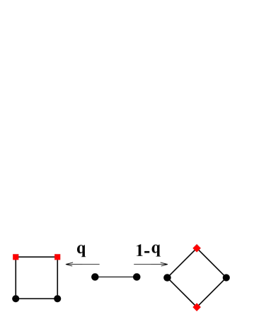
Figure 1: (Color online) Iterative method of the network construction. Each edge is replaced by the connected clusters on the left-hand side with a certain probability $q$, otherwise by the one on the right-hand side, where red squares represent new nodes.

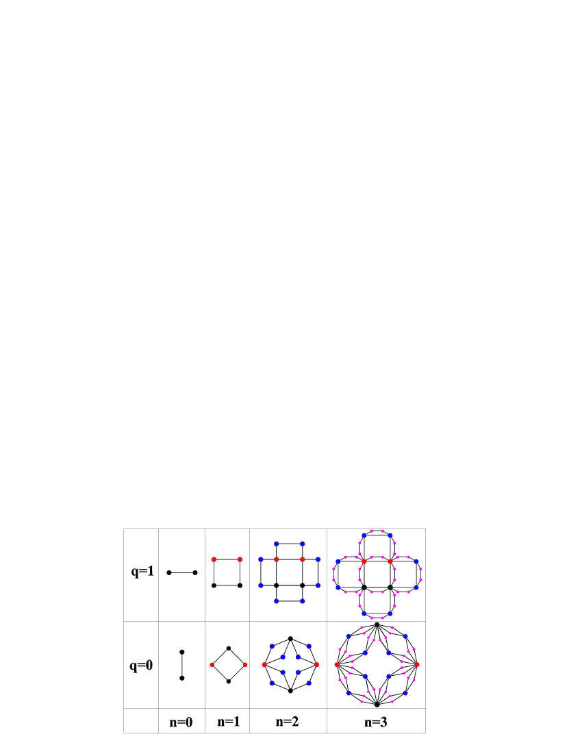
Figure 2: (Color online) Illustration of the first three iterations of the network for the particular cases $q=0$ and $q=1$.

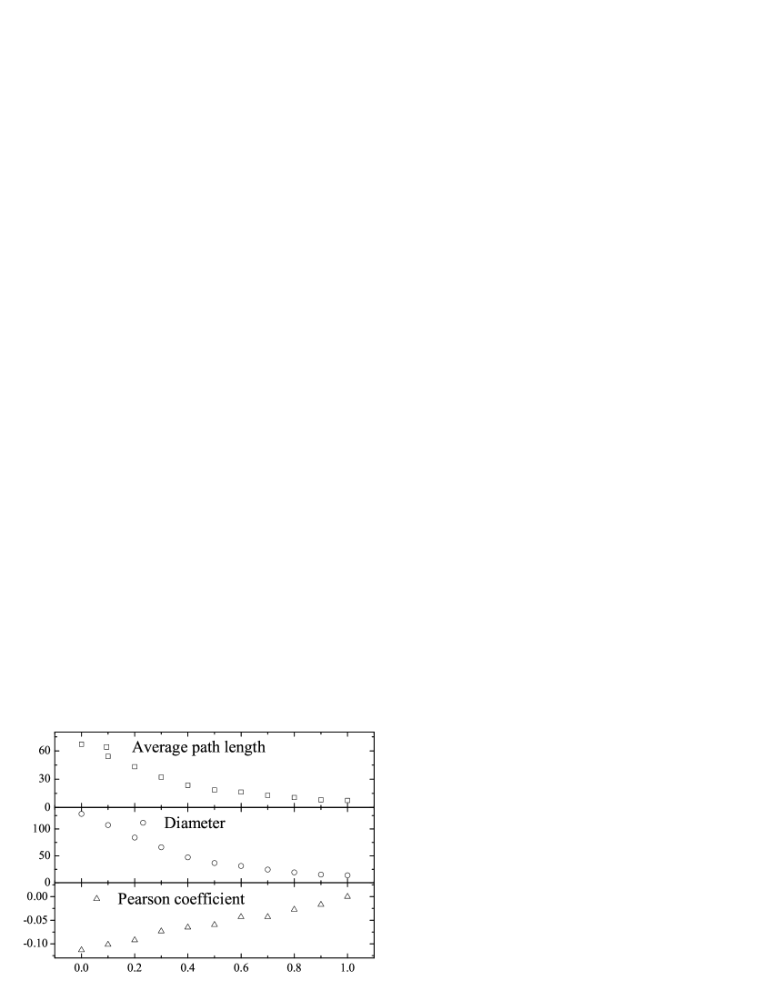
Figure 3: Pearson correlation coefficient, average path length, and diameter versus $q$ ranging from $0$ to $1$ for the IDS-SF networks. Each data point corresponds to ten independent realizations of the network for $n=7$.

4 Diffusion-annihilation processes on the weighted IDS-SF networks

According to the conclusion on the weighted random diffusion operating in the weighted uncorrelated scale-free networks in Section 2, it is easily seen that $P_{i}^{\infty}=\frac{k^{\theta+1}_{i}}{\Sigma_{i}k^{\theta+1}_{i}}$. Thus, for $\theta>0$, particles move towards hubs with time gradually. As hubs are the minority of the population, moving to them means getting concentrated actually. At these hubs, particles have thus a high probability to collide and react with each other, leading to a higher reaction rate than that in homogeneous networks [9]. For $\theta<0$, conversely, the particles are repelled by the hubs. In this case, the particles are getting dispersed on the low-degree nodes with time, which are also called leaves. Seen in this light, reaction rate of diffusion-annihilation tends to decrease with $\theta$ for the two processes. In what follows, we will show the diffusion tendency mentioned above is correct, but the influence of $\theta$ on the reaction rate is not monotonic, which depends not only on degree distribution but also other topological features of the network.

We first generate a special IDS-SF structure through an iterative way with $n=7$. The simulation results are obtained on IDS-SF networks with $10,924$ nodes and $16,384$ links. For the two reaction processes, each node in the networks can host at most one particle. The concrete processes are defined as follows: an arbitrary particle jumps with a certain probability $\frac{w_{ij}}{s_{i}}$ from a node $i$ to a randomly chosen nearest neighbor $j$. If it is empty, the particle fills it, leaving $i$ empty. If $j$ is occupied, the two particles annihilate, leaving both nodes empty. An initial fraction $\rho(0)$ of nodes in the networks is randomly chosen, which is occupied by an $A$ particle with probability $0.5$ for both types. For the $A+B\rightarrow\emptyset$ process, the initial densities of $A$ and $B$ are equal, i.e., $\rho_{B}(0)=\rho_{A}(0)$. For a convenience of discussion, we define $f$ as the first order derivative of $\frac{1}{\rho(t)}$, where $\rho(t)=\rho_{A}(t)$ for $A+A\rightarrow\emptyset$ and $\rho(t)=\rho_{A}(t)+\rho_{B}(t)$ for the $A+B\rightarrow\emptyset$ process. In the cases among $0<q<1$, each plot corresponds to $100$ simulations that are ten runs for ten independent realizations of the network with the same parameters. For the two limiting cases $q=0,1$, each plot corresponds to $100$ runs for the two deterministic networks.

As the degree sequences of the IDS-SF networks with $q\in[0,1]$ are the same, in which $\gamma=3$ [32], Eq. (5) and Eq. (9) can be rewritten as

$$\rho \sim \left\{\begin{array}[]{ccc}t^{-1}&&\theta<0\\ t^{-\frac{1+\theta}{1-\theta}}&&0\leq\theta<1\\ e^{-t}&&\theta\geq 1\end{array}\right..$$ (17)

For the $A+B\rightarrow\emptyset$ process, inserting $\gamma=3$, one can also obtain

$$\rho \sim \left\{\begin{array}[]{ccc}t^{-1}&&\theta<0\\ (t\ln t)^{-1}&&\theta=0\\ t^{-\frac{1}{1-\theta}}&&0<\theta<1\end{array}\right..$$ (21)

For a convenience, we define two quantities as follow:

$$Q_{AA}=\frac{N_{AA}(t)}{M(t)(M(t)-1)},$$ (22)

$$Q_{AB}=\frac{N_{AB}(t)}{M(t)(M(t)-1)},$$ (23)

where $N_{AA}(t)$ denotes the number of close contacts between two nodes with the identical particles for the $A+A\rightarrow\emptyset$ process. $N_{AB}(t)$ denotes the number of contacts between the distinct particles for the $A+B\rightarrow\emptyset$ process at time $t$ [38]. $M(t)$ denotes the total number of particles at time $t$.

4.1 Case of $q=1$

As shown in Fig. 2, in the case $q=1$, the networks are reduced to the $(1,3)$-flower proposed in the reference [35]. By definition [39], the fractal dimension $d_{f}$ can be obtained by

$$d_{f}=\lim_{n\rightarrow\infty}\left(\frac{\ln{N_{n}}}{\ln{l_{n}}}\right),$$ (24)

where $N_{n}$ and $l_{n}$ are the size and diameter of $G_{n}$ respectively. Inserting $N_{n}=\frac{2}{3}(4^{n}+2)$ and $l_{n}=2n$ [35] into Eq. (24), we have

$$d_{f}=\lim_{n\rightarrow\infty}\left(3\ln 2n\right).$$ (25)

Obviously, the net is infinite-dimensional, namely, a non-fractal network.

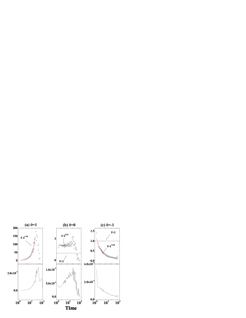
Figure 4: (Color online) $f$ and $Q_{AA}$ as a function of time $t$ for $A+A\to\emptyset$ with $q=1$. The first and second row denote $f$ and $Q_{AA}$ versus $t$ respectively. The dashed lines correspond to the mean field prediction: For the $A+A\to\emptyset$ process, $f=1$ when $\theta=0,-1$, and $f=exp(t)$ when $\theta=1$.

For $A+A\rightarrow\emptyset$, Fig. 4 shows the relation between $f$ and time $t$ for $\theta=-1,0,1$, where red lines are the power-law fittings of the plots. Note that all the plots about the dependence of $f$ and $Q_{AA(AB)}$ on time $t$ are logarithmically binned in this paper. Concretely, $f_{t_{2}}=\frac{\frac{1}{\rho(t_{2})}-\frac{1}{\rho(t_{1})}}{t_{2}-t_{1}}$ and $Q_{t_{2}}=\frac{Q_{t_{2}}-Q_{t_{1}}}{t_{2}-t_{1}}$, where the time interval $log(t_{2})-log(t_{1})=0.1$. For each panel, the curve is relatively stable in the beginning and fluctuates radically in the end. The numerical results show the reaction processes are vastly different from the previous analytical predictions on the weighted uncorrelated networks denoted by the dashed lines [11].

Compared with the mean-field prediction, one can observe many discrepancies in Fig. 4. Here, we only focus on looking for some common reasons. Note that, for $\theta\geq 1$, the mean-field prediction $f=e^{t}$ is much higher than our results in Fig. 4(a). To show the plots clearly, we omit the dashed line in this panel. The apparent discrepancy is mainly caused by the approximation $N_{g}\rightarrow\infty$. In this condition, $\langle k^{1+\theta}\rangle\rightarrow\infty$, which makes the differential equation solvable. For $0<\theta<1$, on the other hand, the approximation in the literature [11] omits the reaction running on the low-degree nodes, which causes the predicted reaction rate is lower than our observation. For $\theta=0$, our results in Fig. 4(b) roughly match the conclusion in the reference [11] in term of the scaling of $f$. But, the value of $f$ is a bit higher than the prediction in that the global mean first-passage time of random walks $G$ in the mean field prediction of Eq. (17) is proportional to $N_{g}$ [40] while $G\sim{N_{g}^{\frac{ln3}{ln4}}}$ [33]. So that, one can expect a larger deviation in the IDS-SF networks with $n>7$. Notably, this observation in this case is inconsistent with the previous conclusion on finite size effects, i.e., $\frac{1}{\rho(t)}\sim N^{\frac{3-\gamma}{2}}t$ for $\gamma\leq 3$ [9]. For $\theta<0$, our results in Fig. 4(c) are basically lower than the prediction. This deviation is caused by the approximation in Taylor expansion. As is known, $\rho(t)$ can only be omitted at the end of the reaction, where it is close to $0$.

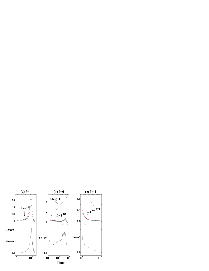
Figure 5: (Color online) $f$ and $Q_{AB}$ as a function of time $t$ for $A+B\to\emptyset$ with $q=1$. The first and second row denote $f$ and $Q_{AB}$ versus $t$ respectively. The dashed lines correspond to the mean field prediction: For $A+B\to\emptyset$, $f=1$ when $\theta=-1$ and $f=ln(t)+1$ when $\theta=0$.

For the $A+B\rightarrow\emptyset$ process, we measure the relation between the total particle density $\rho(t)=\rho_{A}(t)+\rho_{B}(t)$ and time $t$ as shown in Fig. 5. Our observation exhibits the similar behaviors with $A+A\rightarrow\emptyset$. As the probability of collision between two identical particles is equal to that for distinct ones, one can find $Q_{AB}$ in Fig. 5 is about half of the corresponding $Q_{AA}$. Thus, the reaction rate of the $A+B\rightarrow\emptyset$ process is naturally much lower than that of $A+A\rightarrow\emptyset$.

It should be mentioned that the $(1,3)$-flower is a network with a number of common properties, e.g., non-fractal topology, no degree correlations and scale-free degree distribution, satisfying the condition of mean-field approximation fully. But, the annihilation dynamics on it presents many unpredictable properties. Thus, there is a need to provide such a complement to the previous discussion on both fractal scale-free networks [10] and weighted scale-free networks [11]. Without loss of generality, in what follows, we will investigate the other limiting case $q=0$.

4.2 Case of $q=0$

Unlike the case of $q=1$ addressed above, for $q=0$, the networks are reduced to the $(2,2)$-flower as shown in the corresponding panel of Fig. 2, which is a fractal network whose fractal dimension $d_{f}=\frac{\ln 4}{\ln 2}=2$ [35]. By definition, the fractal network is a network satisfying the fractal scaling $N_{B}(l_{B})\sim l_{B}^{d_{f}}$, where $N_{B}$ is the number of boxes needed to cover the entire network with boxes of size $l_{B}$. Note that the fractal scaling $d_{f}$ holds in the system where hubs are located separately from each other [41, 42]. As is known, the mean-field theory can only be applicable when the nets have infinite dimensionality but not in the fractal ones [35, 10]. Thus, the discrepancies between the mean field prediction and our results are not unexpected. However, the weighted networks have their unique subtle properties, which gives rise to many interesting dynamical behaviors distinct from the previous unweighted fractal nets.

For the $A+A\rightarrow\emptyset$ process in Fig. 6, we also measure the relation between $f$ and $t$ for the set of $\theta$. In Fig. 6, one can observe that $f$ decays with time $t$ in all the three panels. In the case of $\theta=1$ in Fig. 6(a), the exponent $f$ decreases with $t$ abnormally and exhibits a contrary behavior with the case of $q=1$, in which $f$ increases with $t$.

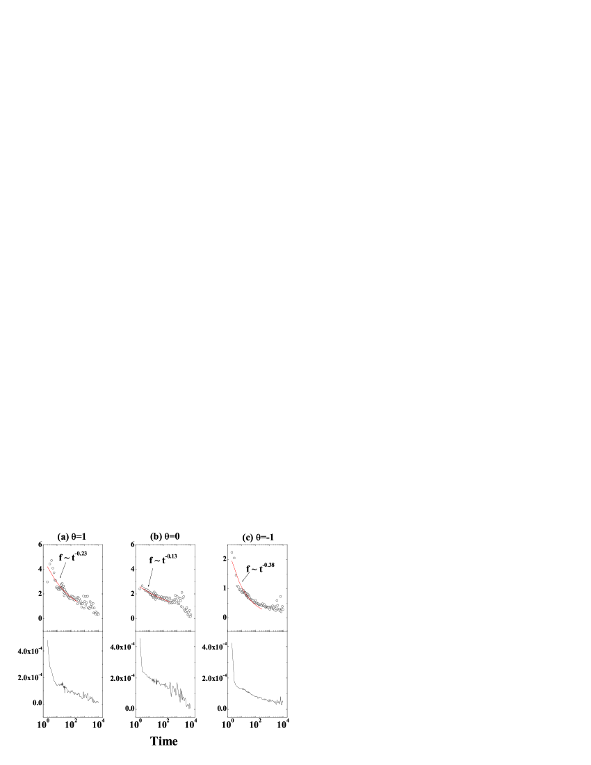
Figure 6: (Color online) $f$ and $Q_{AA}$ as a function of time $t$ for $A+A\to\emptyset$ with $q=0$. The first and second row denote $f$ and $Q_{AA}$ versus $t$ respectively.

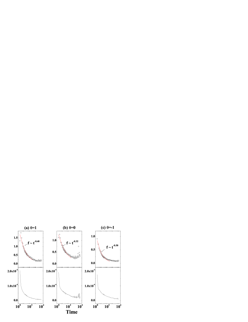
Figure 7: (Color online) $f$ and $Q_{AB}$ as a function of time $t$ for $A+B\to\emptyset$ with $q=0$. The first and second row denote $f$ and $Q_{AB}$ versus $t$ respectively.

For the $A+B\rightarrow\emptyset$ process shown in Fig. 7, one can observe a similar phenomenon with the $A+A\rightarrow\emptyset$ process as well. Because of $Q_{AA}\sim 2Q_{AB}$, $f$ in this case is much lower than the $A+A\rightarrow\emptyset$ as well. Notably, for the unweighted case, i.e., $\theta=0$, $f$ shown in Fig. 7(b) is not a constant $0.5$ mentioned in the reference [10].

For homogeneous initial distributions with equal densities of $A$ and $B$, $\rho_{A}(0)=\rho_{B}(0)$, local hubs and the random fluctuation in the initial particle number generate the segregation of distinct particles, which drastically slows down the reaction rate. Usually, for the unweighted uncorrelated scale-free networks, it is hard for a large number of particles to form a close formation that cannot be penetrated by the other species because of a short diameter. However, for $q=0$, the influence of disassortative mixing is enhanced by the high heterogeneous weight distribution as shown in Fig. 6(a) and Fig. 7(a). The tighter local hubs attract the particles, the lower the diffusion rate is.

As shown in Fig. 8(a), a hub leads to a fast decay of the local $A$ particle density in the beginning, followed by a slow decay in the long time regime as shown in Fig. 6(a). Thus, one can clearly observe depletion zones emerging from the intervals among hubs in this panel. In Fig. 6(b), a hub in a $A$ or $B$-rich domain can give rise to a pure $A$ or $B$ zone after a prompt local annihilation of $A$ and $B$, leaving a relatively particle-free space among the hubs. With these segregations, one can observe a slow decay of the reaction rate as shown Fig. 7(a).

Interestingly, the depletion zone and segregation also inhibit particles moving from leaves to hubs when $\theta<0$. The behavior can be observed by measuring the average degree of occupied nodes increases with $t$ as plotted in Fig. 9. Note that the plots are also logarithmically binned. Recalling the discussion at the beginning of this section, particles are attracted by the leaves in this condition. For $q=1$, particles tend to agglomerate around hubs for $\theta>0$ (see Fig. 9(a)) and leaves for $\theta<0$ (see Fig. 9(c)). Comparing Fig. 4(a) and Fig. 5(a) with Fig. 6(a) and Fig. 7(a), one can figure out the depletion zone and segregation slow down the rate of reaction for $\theta>0$. For $\theta<0$, comparing Fig. 5(c) with Fig. 7(c), instead, they accelerate the rate slightly. This is because they slow down the decentralizing process of the particles. For $\theta=0$, their effect is hardly identified as shown in Fig. 9(b) without the enhancement of weight. Apparently, these interesting behaviors are vastly distinct from the previously reported results [10, 11].

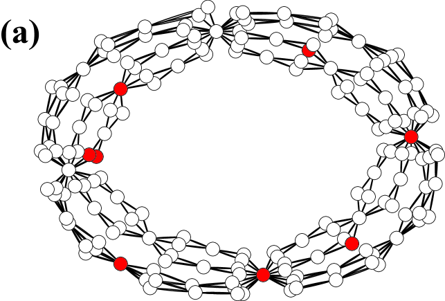
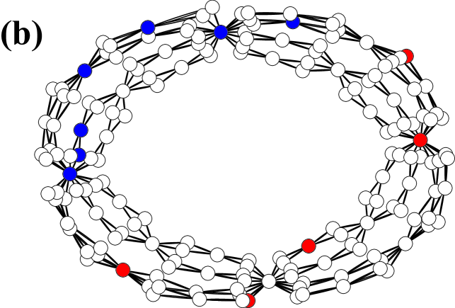
Figure 8: (Color online) Illustration of the $A+A\to\emptyset$ and $A+B\to\emptyset$ processes on the IDS-SF networks with $n=4$. (a) $A+A\to\emptyset$ at $t=10$, and (b) $A+B\to\emptyset$ at $t=15$. Red and blue plots denote $A$ and $B$ particles respectively.

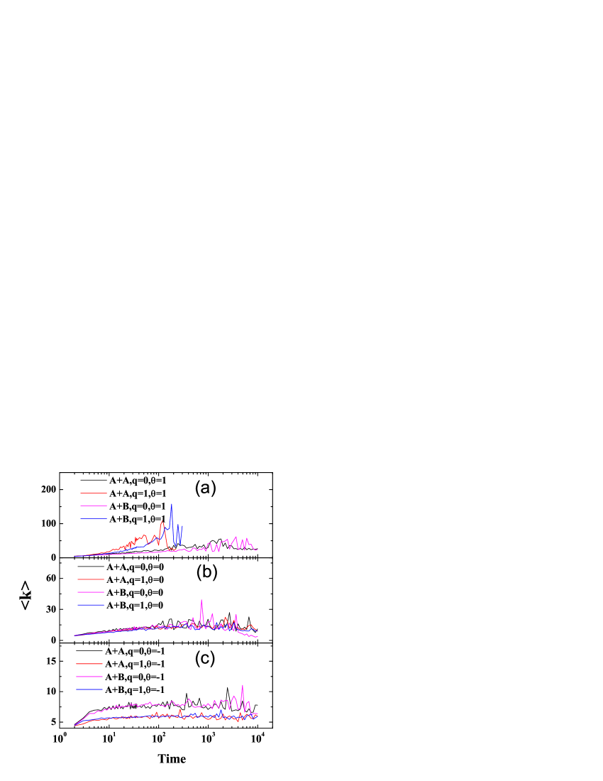
Figure 9: (Color online) $\langle k\rangle$ as a function of time $t$ for $A+A\to\emptyset$ and $A+B\to\emptyset$ for $\theta=-1,0,1$ with $q=0,1$ respectively.

4.3 Case of $0<q<1$

For $0<q<1$, the networks are stochastic, which makes them not self-similar [33]. Thus the networks are non-fractal in this middle case. Thus, in order to discuss the variation in the dependence of $f$ on $q$, we have performed extensive numerical simulations for various $q$ from $0$ to $1$. The simulation settings were the same as the former cases. When $q$ increasing from $0$ to $1$, the exponent of global mean first-passage time of random walks $G(N_{g})$, decreases from $1$ to $\frac{\ln 3}{\ln 4}$ [33], which indicates the enhancement of transporting efficiency during the process. At the same time, the diameter of the networks also decreases while the disassortative mixing feature disappears.

In Fig. 10, one can observe that the segregations among hubs disappear gradually with the increase of $q$. Under the influence, the diffusion rate increases drastically, leading to an apparent enhancement of $f$ for $\theta=1$ (see Fig. 10(a)). Notably, in panel (b), the purely topological segregations for $\theta=0$ are also observable, although its influence is not as apparent as that in panel (a). Also, comparing $q=0.1$ with $q=0.9$, the subtle influence of segregations on the reaction rate in the case of $\theta=-1$ can be identified in panel (c). As shown in this panel, the reaction rate decreases slightly with $q$, which is consistent with our observation in Section 4.2 .

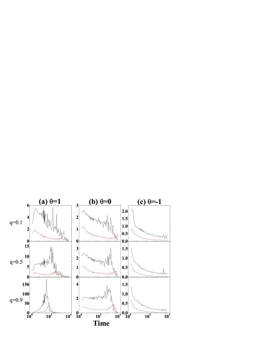
Figure 10: (Color online) Reaction rate exponent $f$ with $\theta=-1,0,1$ and $q=0.1,0.5,0.9$ for $A+A\to\emptyset$ (black lines) and $A+B\to\emptyset$ (red lines) processes on the IDS-SF networks respectively.

5 CONCLUSION

In summary, we have investigated the diffusion-annihilation process on a family of weighted scale-free networks with identical degree sequence (weighted IDS-SF networks), which is controlled by a parameter $q\in[0,1]$. In this paper, the weight of links is defined as $w_{ij}=(k_{i}k_{j})^{\theta}$ with the degree $k_{i}$ and $k_{j}$ of both nodes, where $\theta$ is the network’s weightiness parameter. For a convenience, we define a kinetic exponent $f$ as $\frac{d(\frac{1}{\rho(t)})}{dt}$, where $\rho(t)=\rho_{A}(t)$ for the $A+A\rightarrow\emptyset$ process and $\rho(t)=\rho_{A}(t)+\rho_{B}(t)$ for the $A+B\rightarrow\emptyset$ process. Based on the definition, we provide numerical results to characterize the relation between $f$ and the reaction time $t$ for the $A+A\rightarrow\emptyset$ and $A+B\rightarrow\emptyset$ bimolecular reactions.

One significant observation is that, in contrast to the commonly accepted conception that the depletion zone and segregation only exist in fractal networks. Our observation shows they can exist in the diffusion-annihilation process on the non-fractal networks as well. This striking feature in scale-free networks was not reported in previous studies. In fact, the depletion zone and segregation can both exists in fractal and non-fractal networks no matter whether it is weighted or not. We found that the segregation effect is essentially caused by the disassortative mixing, i.e., high-degree nodes tend to connect with low-degree nodes. On the weighted networks, its influence on the particles diffusion is highly enhanced by the weight heterogeneity. We have demonstrated that both degree and weight distribution do not suffice to characterize the diffusion-annihilation processes on weighted scale-free networks. Our observations suggest care should be taken when making general statements about the diffusion-annihilation process in weighted scale-free networks.

References

References

- [1] R. Albert and A.-L. Barabási, Rev. Mod. Phys. 74, 47 (2002).
- [2] S. N. Dorogvtsev and J. F. F. Mendes, Adv. Phys. 51, 1079 (2002).
- [3] M. E. J. Newman, SIAM Rev. 45, 167 (2003).
- [4] S. Boccaletti, V. Latora, Y. Moreno, M. Chavez, and D.-U. Hwanga, Phys. Rep. 424, 175 (2006).
- [5] F. M. Atay, T. Biyikoǧlu, and J. Jost, IEEE Trans. Circuits Syst., I: Fundam. Theory Appl. 53, 92 (2006).
- [6] A. Hagberg, P. J. Swart, and D. A. Schult, Phys. Rev. E 74, 056116 (2006).
- [7] V. M. Eguíluz and K. Klemm, Phys. Rev. Lett. 89, 108701 (2002).
- [8] L. K. Gallos and P. Argyrakis, Phys. Rev. Lett. 92, 138301 (2004).
- [9] M. Catanzaro, M. Boguñá, and R. Pastor-Satorras, Phys. Rev. E 71, 056104 (2005).
- [10] C. K. Yun, B. Kahng and D. Kim, New J. Phys. 11, 063025 (2009).
- [11] S. Kwon, W. Choi, and Y. Kim, Phys. Rev. E 82, 021108 (2010).
- [12] B. P. Lee, J. Phys. A 27, 2633 (1994).
- [13] U. C. Täuber, M. Howard, and B. P. Lee, J. Phys. A 38, R79 (2005).
- [14] F. Leyvraz and S. Redner, Phys. Rev. A 46, 3132 (1992)
- [15] D. C. Torney and H. M. McConnell, J. Phys. Chem. 87, 1941 (1983); Proc. R. Soc. London A 487, 147 (1983).
- [16] D. Toussaint and F. Wilczek, J. Chem. Phys. 78, 2642 (1983).
- [17] R. Pastor-Satorras, A. V zquez, and A. Vespignani, Phys. Rev. Lett. 87, 258701 (2001).
- [18] A. Vázquez, R. Pastor-Satorras, and A. Vespignani, Phys. Rev. E 65, 066130 (2002).
- [19] A. Barrat, M. Barthélemy, R. Pastor-Satorras, and A. Vespignani, Proc. Natl. Acad. Sci. U.S.A. 101, 3747 (2004).
- [20] A. Fronczak and P. Fronczak, Phys. Rev. E 80, 016107 (2009).
- [21] A. Einstein, Ann. Phys. (Leipzig) 17, 549 (1905); 19, 371 (1906).
- [22] M. Smoluchowski, Ann. Phys. (Leipzig) 21, 756 (1906).
- [23] J. D. Noh and H. Rieger, Phys. Rev. Lett. 92, 118701 (2004).
- [24] F. Jasch and A. Blumen, Phys. Rev. E 63, 041108 (2001).
- [25] L. A. Adamic, R. M. Lukose, A. R. Puniyani, and B. A. Huberman, Phys. Rev. E 64, 046135 (2001).
- [26] R. Guimerá, A. Díaz-Guilera, F. Vega-Redondo, A. Cabrales, and A. Arenas, Phys. Rev. Lett. 89, 248701 (2002).
- [27] S. Lee, S.-H. Yook, and Yup Kim, Phys. Rev. E 74, 046118 (2006).
- [28] S. Lee, S.-H. Yook, and Yup Kim, Physica A 385, 743 (2007).
- [29] A. Fronczak and P. Fronczak, Phys. Rev. E 74, 026121 (2006).
- [30] M. Molloy and B. Reed, Random Struct. Algorithms 6, 161 (1995).
- [31] M. Catanzaro, M. Boguñá, and R. Pastor-Satorras, Phys. Rev. E 71, 027103 (2005).
- [32] Z. Zhang, S. Zhou, T. Zou, L. Chen, and J. Guan, Phys. Rev. E 79, 031110 (2009).
- [33] Z. Zhang, S. Zhou, W. Xie, M. Li, and J. Guan, Phys. Rev. E 80, 061111 (2009).
- [34] M. E. J. Newman, SIAM Rev. 45, 167 (2003).
- [35] H. D. Rozenfeld, S. Havlin, and D. ben-Avraham, New J. Phys. 9, 175 (2007).
- [36] M. E. J. Newman, Phys. Rev. Lett. 89, 208701 (2002).
- [37] A.-L. Barabási and R. Albert, Science 286, 509, (1999).
- [38] L. K. Gallos and P. Argyrakis, J. Phys.: Condens. Matter 19, 065123 (2007).
- [39] D. ben-Avraham and S. Havlin, Diffusion and Reactions in Fractals and Disordered Systems (Cambridge: Cambridge University Press) (2000).
- [40] V. Tejedor, O. Bénichou, and R. Voituriez, Phys. Rev. E 80, 065104 (2009).
- [41] S.-H. Yook, F. Radicchi and H. Meyer-Ortmanns, Phys. Rev. E 72, 045105 (2005).
- [42] C. Song, S. Havlin and H. A. Makse, Nat. Phys. 2, 275 (2006).