COSMOLOGICAL CONSTRAINTS ON THE HIGGS BOSON MASS

Abstract

For a robust interpretation of upcoming observations from PLANCK and LHC experiments it is imperative to understand how the inflationary dynamics of a non-minimally coupled Higgs scalar field with gravity may affect the determination of the inflationary observables. We make a full proper analysis of the WMAP7+SN+BAO dataset in the context of the non-minimally coupled Higgs inflation field with gravity.

For the central value of the top quark pole mass $m_{T}=171.3$GeV, the fit of the inflation model with non-minimally coupled Higgs scalar field leads to the Higgs boson mass in range $143.7\,{\rm GeV}\leq m_{H}\leq 167{\rm GeV}$ (95% CL)
We show that the inflation driven by a non-minimally coupled scalar field to the Einstein gravity leads to significant constraints on the scalar spectral index $n_{S}$ and tensor-to-scalar ratio $R$ when compared with a tensor with similar constraints to form the standard inflation with a minimally coupled scalar field.
We also show that an accurate reconstruction of the Higgs potential in terms of inflationary observables requires an improved accuracy of other parameters of the Standard Model of particle physics such as the top quark mass and the effective QCD coupling constant.

1 Introduction

The primary goal of particle cosmology is to obtain a concordant description of the early evolution of the universe, establishing a testable link between cosmology and particle physics, consistent with both unified field theory and astrophysical and cosmological measurements. On the ground, the Large Hadron Collider (LHC) at CERN is investigating the elementary particle collisions in the TeV energy range, seeking to validate a large number of theoretical predictions of the Standard Model (SM) of particle physics and beyond. In the sky, the PLANCK Surveyor is actively taking precise measurements of the Cosmic Microwave Background (CMB) temperature and polarization anisotropies.

Inflation is the most simple and robust theory capable of explaining astrophysical and cosmological observations, at the same time providing self-consistent primordial initial conditions Starobinsky (1979); Guth (1981); Sato (1981); Albercht (1982); Linde (1982, 1983) and mechanisms for the quantum generation of scalar (curvature) and tensor (gravitational waves) perturbations Mukanov (1981); Hawking (1982); Guth (1982); Starobinsky (1982); Bardeen (1983); Abbot (1984). In the simplest class of inflationary models, inflation is driven by a single scalar field $\phi$ (or inflaton) with some potential $V(\phi)$ minimally coupled to the Einstein gravity. The perturbations are predicted to be adiabatic, nearly scale-invariant and Gaussian distributed, resulting in an effectively flat universe.
The WMAP cosmic microwave background (CMB) measurements alone Dunkley et al. (2009); Larson et al. (2010) or complemented with other cosmological datasets Komatsu et al. (2009, 2010) support the standard inflationary predictions of a nearly flat universe with adiabatic initial density perturbations. In particular, the detected anti-correlations between temperature and E-mode polarization anisotropy on degree scales Nolta et al. (2009) provide strong evidence for correlation on length scales beyond the Hubble radius.

Alternatively, one can look to the inflationary dynamics based on models beyond the Standard Model (SM) of particle physics. The hybrid inflation models involving supersymmetric (SUSY) TeV energy scales Dvali et al. (1994) and minimal supergravity (SUGRA) Linde & Riotto (1997) provide natural connection between cosmology and particle physics Cervantes-Cota & Dehnen ; Şenoğuz & Shafi (2005). The realization of these inflationary scenarios introduces new physics between the electroweak energy scale and the Planck scale, leading to distinct predictions of the main inflationary parameters, such as the spectral index $n_{S}$ of scalar perturbations and the tensor-to-scalar ratio $R$ Rehman et. al (2008); Rehman09 (2009, 2010).
However, a number of recent papers Bezrukov & Shaposhnikov (2008); Barvinsky et al. (2008); Bezrukov et al. (2009, 2009); De Simone et al. (2009); Bezrukov et al. (2009) reported the possibility that the SM of particle physics with an additional non-minimally coupled term of the Higgs field to the gravitational Ricci scalar can give rise to inflation without the need for additional degrees of freedom to the SM. This scenario is based on the observation that the problem of the very small value of Higgs quadratic coupling required by the CMB anisotropy data can be solved if the Higgs inflaton has a large coupling with gravity Futamase & Maeda (1989); Fakir & Unruh (1990); Komatsu & Futamase (1999); Tsujikawa & Gumjudpai (2004); Barvinsky & Kamenshchik (1994).
The resultant Higgs inflaton effective potential in the inflationary domain is effectively flat and can result in a successful inflation for values of the non-minimal coupling constant $\xi\sim 10^{3}-10^{4}$, allowing for cosmological values for the Higgs boson mass in a window in which the electroweak vacuum is stable and therefore sensitive to the field fluctuations during the early stages of the universe Espinosa et al. (2008).

Limits of the validity of Higgs-type inflation have recently been debated by several authors. Specifically, Barbón & Espinosa (2009) argued that the large coupling of Higgs inflaton to the Ricci scalar makes this model invalid beyond the ultraviolet cutoff scale $\Lambda_{\xi}\simeq M_{P}/\xi$ (here $M_{P}=2.4\times 10^{18}$ GeV is the reduced Planck mass) which is below the Higgs field expectation value at $N$ e-foldings during inflation, $h\simeq\sqrt{N}M_{P}/\sqrt{\xi}$. As consequence, at the ultraviolet cutoff scale $\Lambda_{\xi}$ at least one of the cross-sections of different scattering processes hits the unitarity bound Burgess et al. (2009). The fact that the quantum corrections due to the strong coupling to gravity makes the perturbative analysis to break down at energy scales above $\Lambda_{\xi}$ was interpreted as a signature of a new physics, implying higher dimensional operators at energies above $\Lambda_{\xi}$. However, the theory can still be considered valid above $\Lambda_{\xi}$ if one finds some ultraviolet completion or if a very high degree of fine tuning is required, keeping in this way the unwanted contributions of higher dimensional operators small to zero Bezrukov & Shaposhnikov (2009); De Simone et al. (2009).
Recent papers Lerner & McDonald 2010a ; Lerner & McDonald 2010b ; Burgess et al. (2010); Hertzberg (2010) revisit the arguments against Higgs-type inflation addressing the issue of its naturalness with respect to perturbativity and unitarity violation in the Jordan and Einstein frames. It is shown that the apparent breakdown of this theory in the Jordan frame does not imply new physics, but a failure of the perturbation theory in the Jordan frame as a calculational method. These works demonstrate that for inflation based on a single scalar field with large non-minimal coupling, the quantum corrections at high energy scales are small, making the perturbative analysis valid. As consequence, for these models there is no breakdown of unitarity at the energy scale $\Lambda_{\xi}$. In particular, when the single-field Higgs inflation model is analyzed in the Einstein frame there is no breakdown of the theory at energy scales ${\hat{h}}\geq\Lambda_{\xi}$, where ${\hat{h}}$ is the canonically normalized Higgs scalar field in the Einstein frame. However, the inclusion of two or more scalar fields non-minimally coupled with gravity (in particular, the 3 Goldstone bosons of the Higgs doublet) causes unitarity violation in the Einstein frame at $\Lambda_{\xi}$, making the theory unnatural Hertzberg (2010).

The present cosmological constraints on the Higgs mass are based on mapping between the Renormalization Group (RG) flow equations and the spectral index of the curvature perturbations parameterized in terms of the number of ${\it e}$-foldings until the end of inflation, emerging from the analysis of CMB data combined with astrophysical distance measurements. For a robust interpretation of upcoming observations from PLANCK Mandolesi et al. (2010) and LHC Bayatian et al. (2007) experiments it is imperative to understand how the inflationary dynamics of a non-minimally coupled Higgs scalar field may affect the degeneracy of the inflationary observables.
The aim of this paper is to make a full proper analysis of the WMAP 7-year CMB measurements complemented with astrophysical distance measurements Komatsu et al. (2010); Larson et al. (2010) in the context of the non-minimally coupled Higgs inflaton field with gravity. The paper is structured as follows. In Section 2 we compute the power spectra of scalar and tensor density perturbations generated during inflation driven by a single scalar field non-minimally coupled to gravity. In Section 3 we derive the Higgs field equations and compute the RG improved Higgs field potential and in Section 4 we present our main results. In Section 5 we draw our conclusions. Throughout the paper $a$ is the cosmological scale factor ($a_{0}=1$ today), $\kappa^{2}\equiv 8\pi M_{pl}^{-2}$ where $M_{pl}\simeq 1.22\times 10^{19}$ GeV is the present value of the Planck mass, overdots denotes the time derivatives and ${}_{,\varphi}\equiv\partial/\partial\varphi$.

2 COSMOLOGICAL PERTURBATIONS DRIVEN BY A NON-MINIMALLY COUPLED SCALAR FIELD

In this section we compute the power spectra of scalar and tensor density perturbation generated during inflation driven by a single scalar field non-minimally coupled to gravity via the Ricci scalar Fakir & Unruh (1990); Hwang & Noh (1996); Komatsu & Futamase (1998, 1999); Hwang & Noh (2001); Tsujikawa & Gumjudpai (2004) . The general action for these models in the Jordan frame is given by Futamase & Maeda (1989):

$$S_{J}\equiv\int d^{4}x\sqrt{-g}\left[U(\varphi){\it\bf R}-\frac{1}{2}G(\varphi)(\nabla\varphi)^{2}-V(\varphi)\right]\,,$$ (1)

where $U(\varphi)$ is a general coefficient of the Ricci scalar, R, giving rise to the non-minimal coupling, $G(\varphi)$ is the general coefficient of kinetic energy and $V(\varphi)$ is the general potential.
The generalized $U(\varphi)$R gravity theory in Equation (1) includes diverse cases of coupling. For the generally coupled scalar field $U=(\gamma+\kappa^{2}\xi\varphi^{2})$, $G(\varphi)=1$ and $\gamma$ and $\xi$ are constants. The non-minimally coupled scalar field is the case with $\gamma=1$ while the conformal coupled scalar field is the case with $\gamma=1$ and $\xi=1/6$.
The conformal transformation for the action given in Equation (1) can be achieved by defining the Einstein frame metric as:

$$\hat{g}_{\mu,\nu}=\Omega{g}_{\mu,\nu}\,,\hskip 8.5359pt\hskip 8.5359pt\Omega=2\kappa^{2}U(\varphi)\,,$$ (2)

where the quantities in the Einstein frame are marked by caret.

The kinetic energy in the Einstein frame can be made canonical with respect to the new scalar field ${\hat{\varphi}}$, defined through the scalar field propagator suppression factor $s(\hat{\varphi})$ as De Simone et al. (2009); Barvinsky et al. (2009):

$$s(\hat{\varphi})^{-2}=\left(\frac{{\rm d}\hat{\varphi}}{{\rm d}\varphi}\right)^{2}=\frac{1}{2\kappa^{2}}\frac{G(\varphi)U(\varphi)+3U^{2}(\varphi)_{,\varphi}}{U^{2}(\varphi)}\,.$$ (3)

Thus the non-minimal coupling to the gravitational field introduces a modification to the Higgs field propagator by the factor $s(\hat{\varphi})$, acting as back reaction of the gravitational field.
The scalar potential $\hat{V}(\hat{\varphi})$ in the Einstein frame is given by:

$$\hat{V}(\hat{\varphi})=\frac{1}{4\kappa^{4}}\frac{V(\varphi)}{U^{2}(\varphi)}\,,$$ (4)

leading to the following canonical form of the action in the Einstein frame:

$$S_{E}\equiv\int d^{4}x\sqrt{-g}\left[\frac{1}{2\kappa^{2}}{\it\bf R}-\frac{1}{2}(\nabla\hat{\varphi})^{2}-V(\hat{\varphi})\right]\,.$$ (5)

2.1 Background Field Equations

When evaluating the field equations we assume that the background space-time can be written in the form of a flat (k=0) Robertson-Walker line element:

$${\rm d}s^{2}=g_{\mu,\nu}\,{\rm d}x_{\mu}\,{\rm d}x^{\nu} = -{\rm d}t^{2}+a^{2}(t){\rm d}x^{2}$$

$$= \Omega(x)\left(-{\rm d}{\hat{t}}^{2}+\hat{a}^{2}({\hat{t}}){\rm d}x^{2}\right)\,,$$

where $t$ is the cosmic time and $a$ is the cosmological scale factor. From the above equation we obtain:

$${\rm d}\hat{a}=\sqrt{\Omega}\,{\rm d}a\,,\hskip 28.45274pt{\rm d}\hat{t}=\sqrt{\Omega}\,{\rm d}t\,.$$ (7)

Now the Friedmann equation in the Einstein frame can be written as Komatsu & Futamase (1998); Tsujikawa & Gumjudpai (2004):

$$\hat{H}^{2}=\frac{\kappa^{2}}{3}\left[\left(\frac{{\rm d}\hat{\varphi}}{{\rm d}\hat{t}}\right)^{2}+\hat{V}(\hat{\varphi})\right]\,,\\$$ (8)

where:

$$\hat{H}\equiv\frac{1}{\hat{a}}\frac{{\rm d}\hat{a}}{{\rm d}\hat{t}} = \frac{1}{\sqrt{\Omega}}\left[H+\frac{1}{2\Omega}\frac{{\rm d}\Omega}{{\rm d}t}\right]\,,$$ (9)

$$\frac{{\rm d}\hat{\varphi}}{{\rm d}\hat{t}} = \left(\frac{{\rm d}\hat{\varphi}}{{\rm d}\varphi}\right)\left(\frac{{\rm d}t}{{\rm d}\hat{t}}\right)\dot{\varphi}$$ (10)

Equations (9) and (10) are enough to compute the background field evolution in the Einstein frame if the field equations in the Jordan frame are known (see the next section).

2.2 Scalar and Tensor Perturbations

Neglecting the contribution of the decaying modes, the scale dependence of the amplitudes of scalar (S) and tensor (T) perturbations in the Einstein frame are fully governed by the mode equation Mukanov (1981):

$$\frac{{\rm d}^{2}u_{k}}{{\rm d}{\hat{t}}^{2}}+\left(k^{2}-\frac{1}{{z}}\frac{{\rm d}^{2}z}{{\rm d}{\hat{t}}^{2}}\right)u_{k}=0\,,$$ (11)

where $k$ is the comoving wave number of the mode function $u_{k}$. For the case of scalar perturbations we have Hwang (1996); Hwang & Noh (1996, 2001):

$$\frac{1}{z_{S}}\frac{{\rm d}^{2}z_{S}}{{\rm d}{\hat{t}}^{2}}=({\hat{a}}{\hat{H}})^{2}\left[(1+{\hat{\delta}}_{S})(2+{\hat{\delta}}_{S}+\hat{\epsilon})+\frac{\dot{\hat{\delta}}_{S}}{{\hat{a}}{\hat{H}}}\right]\,,$$ (12)

where:

$$z_{S}=\hat{a}\sqrt{{\hat{Q}_{S}}}\,,\hskip 28.45274pt\hat{Q_{s}}=\left(\frac{{\rm d}\hat{\varphi}/{\rm d}\hat{t}}{\hat{H}}\right)^{2}\,.$$ (13)

and slow-roll parameters $\hat{\epsilon}$ and $\hat{\delta}_{S}$ are given by Stewart & Lyth (1993):

$$\hat{\epsilon}=-\frac{{\dot{\hat{H}}}}{\hat{H}^{2}}\,,\hskip 28.45274pt\hat{\delta}_{S}=\frac{{\dot{\hat{Q}}}_{S}}{2\hat{H}\hat{Q}_{S}}\,.$$ (14)

In the case of tensor perturbations Equation (12) has the same form with the following replacements:

$$z_{S}\rightarrow z_{T}=\hat{a}\sqrt{{\hat{Q}_{T}}}\,,\hskip 28.45274pt{\hat{Q}}_{S}\rightarrow{\hat{Q}}_{T}=1\,,\hskip 28.45274pt\hat{\delta}_{S}\rightarrow{\hat{\delta}_{T}}=\frac{{\dot{\hat{Q}}}_{T}}{2\hat{H}\hat{Q}_{T}}=0\,.$$ (15)

The power spectra of scalar and tensor perturbations are given by Copeland et al. (1994):

$${\cal P}_{S}(k)=\frac{k^{3}}{2\pi^{2}}\,\left(\frac{1}{Q_{S}}\right)^{2}\,\frac{|u_{k}|^{2}}{a^{2}}\hskip 22.76228pt{\cal P}_{T}(k)=\frac{16k^{3}}{\pi m^{2}_{pl}}\,\frac{|u_{k}|^{2}}{a^{2}}\,,$$ (16)

and the spectral index of the scalar perturbations $n_{S}$ is obtained as usual as: $n_{s}-1=d\,{\rm ln}{\cal P}_{S}(k)/d\,{\rm ln}k$.

3 HIGGS BOSON AS INFLATON

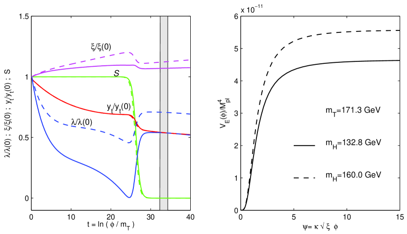
Figure 1: Left panel: The running of the coupling constants normalized to their initial values for $m_{H}=132.8$ GeV (continuous lines) with $\lambda(0)\simeq 0.14$ (blue), $\xi(0)=1.7\times 10^{4}$ (magenta), $m_{H}=160$ (dashed lines) with $\lambda(0)=0.21$ (blue), $\xi(0)=2.1\times 10^{4}$ (magenta) and $m_{T}=171.3$ GeV with $y_{t}(0)=0.91$ (continuous red line). The green curves show the running of the Higgs field propagator suppression factor $s(t)$. The right-hand gray region indicates the slow-roll inflationary regime. Right panel: The Einstein frame renormalization group improved potential as a function of the Higgs field for $m_{H}=132.8$ GeV (continuous line), $m_{H}=160$ (dashed line) and $m_{Top}=171.3$ GeV. In both cases we take the amplitude of scalar perturbations $A^{2}_{S}=2.44\times 10^{-9}$ at the Hubble radius crossing $k_{*}$=0.002 Mpc^-1 and the vacuum expectation value ${\it v}$=246.22 GeV.

Higgs boson as inflaton adds non-minimal coupling to gravity Barvinsky & Kamenshchik (1994); Bezrukov & Shaposhnikov (2008); Barvinsky et al. (2008); De Simone et al. (2009); Bezrukov et al. (2009); Bezrukov & Shaposhnikov (2009).
Taking the Higgs field potential $V(\varphi)$ of the Landau-Ginzburg type (by assuming that the spontaneous symmetry breaking arises through a condensate), the Jordan-frame effective action has the same form as given in Equation (1) with (see e.g. Futamase & Maeda 1989, Fakir & Unruh 1990, Makino & Sasaki 1991):

$$U(\varphi)=\frac{1+\kappa^{2}\xi\varphi^{2}}{2\kappa^{2}}\,,\hskip 42.67912ptV(\varphi)=\frac{\lambda}{4}\left(\varphi^{2}-{\it v}^{2}\right)^{2}\,,\hskip 42.67912ptG(\varphi)=1\,,$$ (17)

where: ${\it v}=(\sqrt{2}G_{F})^{-1/2}$=246.22 GeV is the vacuum expectation value of the Higgs field that sets the electroweak scale, $\lambda$ is the quadratic coupling constat of the Higgs boson with a mass $m_{H}=\sqrt{2\lambda}{\it v}$ and $\xi$ is the non-minimal coupling constant. The Jordan-frame field equations from the above action are given by Komatsu & Futamase (1999); Kaiser (1995):

$$H^{2}=\frac{\kappa^{2}}{3\,(1+\kappa^{2}\xi\phi^{2})}\left[V(\varphi)+\frac{1}{2}\dot{\varphi}^{2}-6\,\xi H\varphi\dot{\varphi}\right]\,,$$ (18)

$$\ddot{\varphi}+3H\dot{\varphi}+\left(\frac{\kappa^{2}\xi\varphi^{2}(1+6\xi)}{1+\kappa^{2}\xi\varphi^{2}(1+6\xi)}\right)\frac{\dot{\varphi}^{2}}{\varphi}=\frac{\kappa^{2}\xi\varphi V(\varphi)-(1+\kappa^{2}\xi\phi^{2})V_{,\,\varphi}(\varphi)}{1+\kappa^{2}\xi\varphi^{2}(1+6\xi)}\,,$$ (19)

which in the slow-roll approximation ( $|\dot{\varphi}/\varphi|\ll H$ and $|\dot{\varphi}^{2}|\ll V(\varphi)$ ) can be written as:

$$H^{2} \simeq \frac{\kappa^{2}}{3(1+\kappa^{2}\xi\phi^{2})}V(\varphi)\,,$$ (20)

$$3H\dot{\varphi} \simeq \frac{\kappa^{2}\xi\varphi V(\varphi)-(1+\kappa^{2}\xi\phi^{2})V_{,\,\varphi}(\varphi)}{1+\kappa^{2}\xi\varphi^{2}(1+6\xi)}\,.$$ (21)

The quantum corrections due to the interaction effects of the SM particles with Higgs boson through quantum loops modify the action coefficients $U(\varphi)$, $V(\varphi)$ and $G(\varphi)$ from their classical expression given in Equations (1) and (17), taking the renormalization group (RG) improved forms $U_{q}(t)$, $V_{q}(t)$, $G_{q}(t)$ defined as Barvinsky et al. (2008); De Simone et al. (2009); Clark et al. (2009); Lerner & McDonald (2009):

$$U_{q}(t) = \frac{1}{2\kappa^{2}}\left(1+\kappa^{2}\xi(t)G_{q}^{2}(t)\varphi(t)^{2}\right)\,,$$ (22)

$$V_{q}(t) = \frac{\lambda(t)}{4}G_{q}^{4}(t)\left(\varphi^{2}(t)-{\it v}^{2}(t)\right)^{2}\,,$$ (23)

$$G_{q}(t) = e^{-\gamma(t)/(1+\gamma(t))}\,,$$ (24)

where $\gamma(t)$ is the Higgs field anomalous dimension given in the Appendix.
The scaling variable $t={\rm ln}(\varphi/m_{T})$ in the above equations normalizes the Higgs field and all the running couplings to the top quark mass scale $m_{T}$.

As the energy scale of inflation is many order of magnitude above the electroweak scale ($\varphi(t)>>{\it v}$), in the following we will approximate the Higgs potential by $V(\varphi)\simeq\lambda\varphi^{4}/4$, neglecting the vacuum contribution and its running in the potential.
Making the conformal transformation (2), Equations (3) and (4) yield to:

$$s(t)^{-2}=\left(\frac{{\rm d}\hat{\varphi}(t)}{{\rm d}\varphi(t)}\right)^{2} = \frac{1}{2\kappa^{2}}\,\frac{1+\kappa^{2}\xi(t)\varphi^{2}(t)(1+6\xi(t))}{(1+\kappa^{2}\xi(t)\varphi^{2}(t))^{2}}\,,$$ (25)

$$\hat{V}(t) = \frac{1}{16\kappa^{4}}\,\frac{\lambda(t)\varphi^{4}(t)}{(1+\kappa^{2}\xi(t)\varphi^{2}(t))^{2}}\,.$$ (26)

The amplitude of scalar density perturbations at the Hubble radius crossing $k_{*}$ is then given by:

$$A^{2}_{S}=\left.\frac{{\hat{V}}}{24\pi^{2}M^{2}_{pl}\epsilon}\right|_{k_{*}}\,,\hskip 42.67912pt\epsilon=\frac{1}{2}M^{2}_{pl}\left(\frac{\hat{V}_{\,,\varphi}}{\hat{V}}\right)^{2}\,.$$ (27)

We compute the various $t$-dependent running constants, the Higgs field propagator suppression factor and the Higgs field anomalous dimension by integrating the RG $\beta$-functions as compiled in the Appendix. The runnings of $SU(2)\times S(1)$ gauge couplings ${g^{\prime},g}$, the $SU(3)$ strong coupling $g_{s}$, the top Yukawa coupling $y_{t}$ and the Higgs quadratic coupling $\lambda$ are computed by using two-loop quantum corrections while the running of non-minimal coupling constant $\xi$ is computed by using one-loop quantum corrections.
One should note the importance of the quantum corrections due to non-minimal coupling. The quantum corrections to the classical kinetic sector $G(\varphi)=1$ arise from the Higgs field anomalous dimension $\gamma(t)$ occurring with a factor of $1/\xi$ which in the inflationary regime ($\xi\sim 10^{4}$) has a negligible small contribution. In the case of a classical gravity sector $U(\varphi)=(1+\kappa^{2}\xi\varphi^{2})/2\kappa^{2}$, the conformal transformation (2) introduces a one-loop $\beta$-function for $\xi$ with a term proportional to $\lambda$ due to Higgs running in a loop which has a small contribution during inflation due to the suppression of the Higgs field propagator, while the contribution of the remaining terms cancel to good approximation De Simone et al. (2009). Although small, the one-loop quantum corrections due to the non-minimal coupling are not negligible but enough for the purpose of this analysis.

For each case, the $t$-dependent running constants are obtained as:

$$Y(t)=\int^{t}_{t=0}\frac{\beta_{Y}(t^{\prime})}{1+\gamma(t^{\prime})}\,{\rm d}t^{\prime}\,,\hskip 42.67912ptY=\{g,g^{\prime},g_{s},y_{t},\lambda,\xi\}\,,$$ (28)

At $t=0$, which corresponds to the top quark mass scale $m_{T}$, the Higgs quadratic coupling $\lambda(0)$ and the top Yukawa coupling $y_{t}(0)$ are determined by the pole masses and the vacuum expectation value ${\it v}$:

$$\lambda(0)=\frac{m^{2}_{H}}{2{\it v}^{2}}\left[1+\Delta_{H}(m_{H})\right]\,,\hskip 42.67912pty_{t}(0)=\frac{\sqrt{2}m_{T}}{\it v}\left[1+\Delta_{T}(m_{T})\right]\,,$$ (29)

where $\Delta_{H}(m_{H})$ and $\Delta_{T}(m_{T})$ are the corrections to Higgs and top quark mass respectively, computed following the scheme from the Appendix of Espinosa et al. (2008).
The gauge coupling constants at $m_{T}$ scale are Barvinsky et al. (2009): $g^{2}(0)=0.4202$, $g^{\prime 2}(0)=0.1291$ and $g^{2}_{s}(0)=1.3460$. The value of the non-minimal coupling constant $\xi(0)$ is determined so that at the beginning of the slow-roll inflation $t_{ini}$ the non-minimally coupling constant $\xi(t_{ini})$ is such that the calculated value of the amplitude of density perturbations given in Equation (27) agrees with the measured value of $A^{2}_{S}$.
Figure 1 presents the running of the coupling constants and of the Higgs field propagator suppression factor obtained for two different values of the Higgs boson mass. In both cases we also show the Einstein frame renormalization group improved potential as a function of the Higgs field $\psi=\kappa\sqrt{\xi}\varphi(t)$.

4 Results

4.1 The CMB Angular Power Spectra

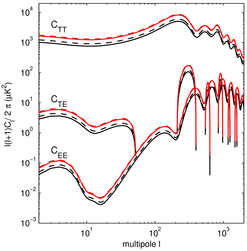
Figure 2: The renormalization group improved CMB temperature and polarization angular power spectra (continuous lines) compared with the same power spectra obtained at the tree-level (dashed-lines) for $m_{H}$=145 GeV (black lines) and $m_{H}$=160 GeV (red lines). In both cases we take the top quark pole mass $m_{T}=171.3$ GeV, the amplitude of scalar perturbations $A^{2}_{S}=2.44\times 10^{-9}$ at Hubble radius crossing $k_{*}$=0.002 Mpc^-1 and the vacuum expectation value ${\it v}$=246.22 GeV.

We obtain the CMB temperature anisotropy and polarization power spectra by integrating the coupled Equations (9), (10) and (11) together with Equations (20) and (21) with respect to the conformal time imposing that the electroweak vacuum expectation value ${\it v}=$246.22 GeV is the true minimum of the Higgs potential at any energy scale ($\lambda(t)>$0). We take wavenumbers in the range [$5\times 10^{-6}-5$] Mpc^-1 needed by the CAMB Boltzmann code Lewis et al. (2000) to numerically derive the CMB angular power spectra and a Hubble radius crossing scale $k_{*}=0.002$Mpc^-1. The value of the Higgs scalar field $\varphi_{*}$ at this scale is related to the quantum scale of inflation $\varphi_{I}$ and to the duration of inflation expressed in units of e-folding number ${\it N}$ through Barvinsky et al. (2008):

$$\frac{\varphi^{2}_{*}}{\varphi_{I}} = e^{x}-1\,,\hskip 42.67912pt\varphi^{2}_{I}=\frac{64\pi^{2}M^{2}_{pl}}{\xi{\bf A_{I}}}\,,\hskip 42.67912ptx\equiv\frac{{\it N}{\bf A_{I}}}{48\pi^{2}}\,,$$ (30)

$${\bf A_{I}} = \frac{3}{8\lambda}\left(2g^{4}+(g^{2}+g^{\prime 2})^{2}-16y_{t}^{4}\right)-6\lambda\,,$$ (31)

where the inflationary anomalous scaling parameter ${\bf A_{I}}$ Barvinsky & Kamenshchik (1994); Barvinsky et al. (2009) involves a special combination of quantum corrected coupling constants. These relations determine the value of the scaling parameter $t_{*}={\rm ln}(\varphi_{*}/m_{T})$ at Hubble radius crossing $k_{*}$. As the inflationary observables are evaluated at the epoch of horizon-crossing quantified by the number of e-foldings $N$ before the end of the inflation at which our present Hubble scale equalled the Hubble scale during inflation, the uncertainties in the determination of $N$ translates into theoretical errors in determination of the inflationary observables Kinney et al. (2004); Kinney & Riotto (2006). Assuming that the ratio of the entropy per comoving interval today to that after reheating is negligible, the main uncertainty in the determination of $N$ is given by the uncertainty in the determination of the reheating temperature after inflation. Recent studies of the reheating after inflation driven by SM Higgs field non-minimally coupled with gravity estimates the reheating temperature in the range Garcia-Bellido et al. (2009); Bezrukov et al. (2009):

$$3.4\times 10^{13}\,{\rm GeV}<T_{r}<\left(\frac{\lambda}{0.25}\right)^{1/4}\,1.1\times 10^{14}\,{\rm GeV}\,,$$

which translates into a negligible variation of the number of e-foldings with the Higgs mass ($\Delta~{}N~{}\sim~{}0.1$). For the purpose of this work we choose ${\it N}=k_{*}/aH=$ 59 ${\it e}$-foldings in view of WMAP7+SN+BAO normalization at $k_{*}$ Komatsu et al. (2010); Larson et al. (2010).
For each wavenumber $k$ in the above range our code integrates the $\beta$-functions of the $t$-dependent running constant couplings in the observational inflationary window imposing that $k$ grows monotonically to the wavenumber $k_{*}$, at the same time eliminating those models violating the condition for inflation $0\leq\epsilon_{H}\equiv-{\dot{H}}/H^{2}\leq 1$.
Figure 2 presents the RG improved CMB temperature and polarization power spectra compared with the same power spectra obtained at the tree-level for $m_{H}$=145 GeV and $m_{H}$=160 GeV. These plots clearly show that the CMB anisotropies are sensitive to the quantum radiative corrections of the SM coupling constants.

4.2 Markov Chain Monte Carlo (MCMC) Analysis

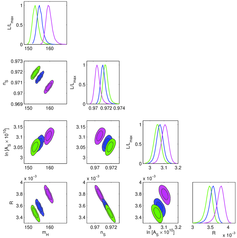
Figure 3: The results of the fit of inflationary model with a non-minimal coupled Higgs scalar field to the WMAP7+SN+BAO dataset for top quark pole mass values: 168 GeV (green), 171.3 GeV (blue) and 173 GeV (magenta). The top plot in each column shows the probability distribution of different parameters while the other plots show their joint 68% and 95% confidence intervals. All parameters are computed at the Hubble crossing scale $k_{*}$=0.002Mpc^-1.

We use MCMC technique to reconstruct the Higgs field potential and to derive constraints on the inflationary observables and the Higgs mass from the following datasets.
The WMAP 7-year data Komatsu et al. (2010); Larson et al. (2010) complemented with geometric probes from the Type Ia supernovae (SN) distance-redshift relation and the baryon acoustic oscillations (BAO). The SN distance-redshift relation has been studied in detail in the recent unified analysis of the published heterogeneous SN data sets - the Union Compilation08 Kowalski et al. (2008); Riess et al. (2009). The BAO in the distribution of galaxies are extracted from Two Degree Field Galaxy Redshidt Survey (2DFGRS) the Sloan Digital Sky Surveys Data Release 7 Percival et al. (2010). The CMB, SN and BAO data (WMAP7+SN+BAO) are combined by multiplying the likelihoods. We use these measurements especially because we are testing models deviating from the standard Friedmann expansion. These datasets properly enables us to account for any shift of the CMB angular diameter distance and of the expansion rate of the Universe.
The likelihood probabilities are evaluated by using the public packages CosmoMC and CAMB Lewis & Briddle (2002); Lewis et al. (2000) modified to include the formalism for inflation driven by non-minimally coupled Higgs scalar field as described in the previous sections. Our fiducial model is the $\Lambda$CDM standard cosmological model described by the following set of parameters receiving uniform priors:

$$\left\{\Omega_{b}h^{2}\,,\,\,\Omega_{c}h^{2}\,,\,\,\theta_{s}\,,\,\,\tau\,,\,\,A^{2}_{S}\,,\,\,m_{H}\,,\,\,m_{T}\right\}\,,$$

where: $\Omega_{b}h^{2}$ is the physical baryon density, $\Omega_{c}h^{2}$ is the physical dark matter density, $\theta_{s}$ is the ratio of the sound horizon distance to the angular diameter distance, $\tau$ is the reionization optical depth, $A^{2}_{S}$ is the amplitude of scalar density perturbations, $m_{H}$ is the Higgs boson pole mass and $m_{T}$ is the top quark pole mass. For comparison we use the MCMC technique to reconstruct the standard inflation field potential and to derive constraints on the inflationary observables from the fit to WMAP7+SN+BAO dataset of the standard inflation model with minimally coupled scalar field. For this case we use the same set of input parameters with uniform priors as in the case of non-minimally coupled Higgs scalar field inflation, except for Higgs boson and top quark pole masses. The details of this computation can be found in Popa et al. (2009).
For each inflation model we run 64 Monte Carlo Markov chains, imposing for each case the Gelman & Rubin convergence criterion Gelman & Rubin (1992). Figure 3 presents the constraints on the Higgs boson mass $m_{H}$, the spectral index of the scalar density perturbations $n_{S}$, the amplitude of the scalar density perturbations $A^{2}_{S}$ and the ratio of tensor-to-scalar amplitudes $R$, as obtained from the fit to the WMAP7+SN+BAO dataset of the inflation model with non-minimally coupled Higgs scalar field for three different top quark pole mass values. We find that $n_{S}$, $A^{2}_{S}$ and R are dependent of the Standard Model parameters, in particular on the Higgs quadratic coupling and Yukawa coupling. One should recall that in the standard inflation these parameters are independent on the parameters of the Standard Model.
The running of Higgs quadratic coupling $\lambda$ is increased for a heavier Higgs, also receiving contributions from gauge couplings $\{g,g^{\prime},g_{s}\}$ and top Yukawa coupling $y_{t}$. In the inflationary regime, the contribution from $y_{t}$ is increased as the top quark mass is varied toward higher mass values through its experimental allowed range: 168 GeV - 173 GeV Amsler et al. (2008). As a consequence, since we fixed the non-minimal coupling constant $\xi$ such that the amplitude of the scalar density perturbations $A^{2}_{S}\sim\lambda/\xi^{2}$ is at the observed value, $A^{2}_{S}$ increases for a heavier Higgs boson and a higher top quark mass value, leading to the suppression of the spectral index of scalar density perturbations $n_{s}$. Moreover, the joint confidence regions of the scalar spectral index $n_{s}$ and of the ratio of tensor-to-scalar amplitudes $R$ are anti-correlated. This can be attributed to a larger contribution of the tensor modes to the primordial density perturbations when Higgs boson and top quark masses are increased. Table 1 presents the mean values and the errors (68% CL) of the parameters from the posterior distributions obtained from the fit of the standard inflation model and the inflation model with non-minimally coupled Higgs scalar field with $m_{T}$=171.3 GeV and ${\it v}$=246.22 GeV to WMAP7+SN+BAO dataset. We find for Higgs boson pole mass the following dependence on $m_{T}$ and $\alpha_{s}(m_{Z})$ normalized in units of one standard deviations from their experimental central values:

$$m_{H} \simeq (155.37\pm 3.85\pm\delta)\,{\rm GeV}+3.8\,{\rm GeV}\left(\frac{m_{T}-171.3\,{\rm GeV}}{2.3\,{\rm GeV}}\right)$$ (32)

$$- 1.4\,{\rm GeV}\left(\frac{\alpha_{s}(m_{Z})-0.1176}{0.0020}\right)\hskip 19.91684pt(68\%{\rm\,\,\,CL)}\,,$$

where we included the overall theoretical uncertainty $\delta\simeq 2$ GeV accounting for higher-order quantum corrections Espinosa et al. (2008).

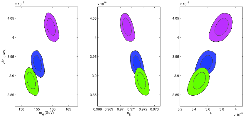
Figure 4: The dependence of the reconstructed Higgs field potential (the joint 68% and 95% confidence intervals) on $m_{H}$, $n_{S}$ and $R$ as obtained from the fit of inflationary model with non-minimally coupled Higgs scalar field to the WMAP7+SN+BAO dataset for top quark pole mass values: 168 GeV (green), 171.3 GeV (blue) and 173 GeV (magenta). All parameters are computed at the Hubble crossing scale $k_{*}$=0.002Mpc^-1.

In Figure 4 we present the dependence of the recovered Higgs field potential on $m_{H}$, $n_{S}$ and $R$ as obtained from the fit of inflationary model with non-minimally coupled Higgs scalar field to the WMAP7+SN+BAO dataset for different top quark pole mass values. Figure 4 explicitly demonstrates that the cosmological measurements not only probe the graviton-inflaton sector of the SM but also the variation of the scale of inflation due to the SM heavy particles coupled to inflation.

5 CONCLUSIONS

A number of papers have discussed bounds on the Higgs boson mass coming from demanding stability or metastability of the lifetime of the universe Espinosa et al. (2008). Further, by demanding that Higgs drive inflation, depending on the top quark mass and the computation of the RG improved effective potential, it was found that a heavier Higgs boson with a mass within the absolute stability bounds is required Bezrukov & Shaposhnikov (2008); Barvinsky et al. (2008); Bezrukov et al. (2009, 2009); De Simone et al. (2009); Bezrukov et al. (2009). However, the present cosmological constraints on the Higgs boson mass are based on mapping between the RG flow and the scalar spectral index of of curvature perturbations.
For a robust interpretation of upcoming observations from PLANCK Mandolesi et al. (2010) and LHC Bayatian et al. (2007) experiments it is imperative to understand how the inflationary dynamics of a non-minimally coupled Higgs scalar field with gravity may affect the determination of the inflationary observables. The aim of this paper is to make a full proper analysis of the WMAP 7-year CMB measurements Komatsu et al. (2010); Larson et al. (2010) complemented with geometric probes from the Type Ia supernovae (SN) distance-redshift relation Kowalski et al. (2008); Riess et al. (2009) and the baryon acoustic oscillations (BAO) in the distribution of galaxies from Two Degree Field Galaxy Redshidt Survey (2DFGRS) and the Sloan Digital Sky Surveys Data Release 7 Percival et al. (2010), in the context of the non-minimally coupled Higgs inflaton with gravity.
We compute the full RG improved effective potential including two-loop beta functions for $SU(2)\times S(1)$ gauge couplings ${g^{\prime},g}$, the $SU(3)$ strong coupling $g_{s}$, the top Yukawa coupling $y_{t}$ and the Higgs quadratic coupling $\lambda$ and one-loop beta functions for non-minimal coupling constant $\xi$ and vacuum expectation value v. We also include the curvature in RG flow equations through Higgs field propagator suppression function $s(t)$ and the Higgs field anomalous dimension $\gamma(t)$.
The initial conditions for $\lambda$ and $y_{t}$ are properly obtained through the pole mass matching scheme while the inflationary anomalous scale parameter ${\bf A_{I}}$ relates the initial value of the Higgs inflation field to the quantum scale of inflation and the number of e-foldings.
We use MCMC technique to reconstruct the Higgs field potential and to derive constraints on the inflationary observables and the Higgs mass from WMAP7+SN+BAO dataset. For the central value of the top quark pole mass $m_{T}=171.3$GeV the fit of the inflation model with non-minimally coupled Higgs scalar field to WMAP7+SN+BAO dataset leads to the following 95% CL bounds on Higgs boson mass:

$$143.7\,{\rm GeV}\leq m_{H}\leq 167.0\,{\rm GeV}\,,$$ (33)

where we take into account the overall theoretical error $\delta=\pm 2$ GeV and $\alpha_{s}(m_{Z})=0.1176$.
We show that the inflation driven by a non-minimally coupled scalar field to the Einstein gravity leads to significant constraints on the scalar spectral index $n_{S}$ and tensor-to-scalar ratio $R$, when compared with the similar constraints from the standard inflation with minimally coupled scalar field. In particular, one should note the smallness of tensor-to-scalar ratio ($R\sim 10^{-3}$) that is challenging the future polarization experiments.
We conclude that in order to obtain an accurate reconstruction of the Higgs potential in terms of inflationary observables it is imperative to improve the accuracy of other parameters of the SM as the top quark mass and the effective QCD coupling constant.
For example, it is expected that in the near future LHC will improve the determination of the current value of top quark mass to $\Delta m_{T}\simeq 1.5$ GeV. From Equation (32) it follows that this improvement will lead to an improvement in the determination of the Higgs boson mass to $\Delta m_{T}\simeq 2.4$ GeV. Since $A^{2}_{S}\sim\lambda$, using Equation (27) with $R=16\epsilon$ and fixing all parameters at their observed values, it follows that the expected improved determination of the top quark mass leads to an improved accuracy in the determination of the Higgs potential of about 3%.

Table 1: The mean values from the posterior distributions of the parameters obtained from the fit of the standard inflation model and Higgs inflation model with $m_{T}$=171.3 GeV and ${\it v}$=246.22 GeV to WMAP7+SN+BAO dataset. The errors are quoted at 68% CL. All parameters are computed at the Hubble radius crossing $k_{*}$=0.002 Mpc^-1.

Model	Standard Inflation	Higgs Inflation
Parameter
$100\Omega_{b}h^{2}$	2.259$\pm$0.054	2.257$\pm$0.051
$\Omega_{c}h^{2}$	0.113$\pm$0.003	0.114$\pm$0.003
$\tau$	0.088$\pm$0.015	0.086$\pm$0.013
$\theta_{s}$	1.038$\pm$0.002	1.037$\pm$0.002
${\rm ln}[10^{10}A^{2}_{S}]$	3.157$\pm$0.031	3.161$\pm$0.032
$n_{S}$	0.960$\pm$0.012	0.972$\pm$0.0004
R	$<$ 0.144	0.0036$\pm$0.0009
$m_{H}$(GeV)	-	155.372$\pm$3.851
$\lambda$	-	0.216$\pm$0.053
$\xi\times 10^{-4}$	-	3.147 $\pm$ 0.509

Acknowledgments

The authors acknowledge the referee the useful comments.// This work was partially supported by CNCSIS Contract 539/2009 and by ESA/PECS Contract C98051.

6 APPENDIX

In this appendix we collect the SM renormalization group $\beta$-functions Ford et al. (1992), including the Higgs field propagator suppression factor $s(t)$ given in Equation (25), at the renormalization energy scale $t={\rm ln}(\varphi/m_{t})$ beyond the top quark mass $m_{t}$.
The two-loop $\beta$-functions for gauge couplings $g_{i}=\{g^{\prime},g,g_{s}\}$ are Espinosa et al. (2008):

$$\beta_{g_{i}} = kg_{i}^{3}b_{i}+k^{2}g_{i}^{3}\left[\sum_{j=1}^{3}B_{ij}g_{j}^{2}-s(t)d_{i}^{t}y_{t}^{2}\right],$$ (34)

where $k=1/16\pi^{2}$ and

$$b=((40+s(t))/6,-(20-s(t))/6,-7),\quad B = \left(\begin{array}[]{ccc}199/18&9/2&44/3\\ 3/2&35/6&12\\ 11/6&9/2&-26\end{array}\right),$$ (38)

$$d^{t}=(17/6,3/2,2).$$ (39)

For the top Yukawa coupling $y_{t}$, the two-loop $\beta$-function is given by De Simone et al. (2009):

$$\beta_{y_{t}} =k\,y_{t}\left[-\frac{9}{4}g^{2}-\frac{17}{12}g^{\prime 2}-8g^{2}_{s}+\frac{9}{2}s(t)y_{t}^{2}\right]+k^{2}y_{t}\Bigg{[}-\frac{23}{4}g^{4}-\frac{3}{4}g^{2}g^{\prime 2}+\frac{1187}{216}g^{\prime 4}+9g^{2}g_{s}^{2}$$

$$+ \frac{19}{9}g^{\prime 2}g_{s}^{2}-108g_{s}^{4}+\left(\frac{225}{16}g^{2}+\frac{131}{16}g^{\prime 2}+36g_{s}^{2}\right)s(t)y_{t}^{2}+6\left(-2s^{2}(t)y_{t}^{4}-2s^{3}(t)y_{t}^{2}\lambda+s^{2}(t)\lambda^{2}\right)\Bigg{]}\,.$$

The two-loop $\beta$-function for the Higgs quadratic coupling $\lambda$ is De Simone et al. (2009):

$$\beta_{\lambda} = k\left[24s^{2}\lambda^{2}-6y_{t}^{4}+\frac{3}{8}\left(2g^{4}+\left(g^{2}+g^{\prime 2}\right)^{2}\right)+\left(-9g^{2}-3g^{\prime 2}+12y_{t}^{2}\right)\lambda\right]$$ (41)

$$+ k^{2}\Bigg{[}\frac{1}{48}\left(915g^{6}-289g^{4}g^{\prime 2}-559g^{2}g^{\prime 4}-379g^{\prime 6}\right)+30s(t)y_{t}^{6}-y_{t}^{4}\left(\frac{8g^{\prime 2}}{3}+32g_{s}^{2}+3s(t)\lambda\right)$$

$$+ \lambda\left(-\frac{73}{8}g^{4}+\frac{39}{4}g^{2}g^{\prime 2}+\frac{629}{24}s(t)g^{\prime 4}+108s^{2}(t)g^{2}\lambda+36s^{2}(t)g^{\prime 2}\lambda-312s^{4}(t)\lambda^{2}\right)$$

$$+ y_{t}^{2}\left(-\frac{9}{4}g^{4}+\frac{21}{2}g^{2}g^{\prime 2}-\frac{19}{4}g^{\prime 4}+\lambda\left(\frac{45}{2}g^{2}+\frac{85}{6}g^{\prime 2}+80g_{s}^{2}-144s^{2}(t)\lambda\right)\right)\Bigg{]}.$$

The one-loop $\beta$-function for non-minimal coupling $\xi$ is given by Bezrukov & Shaposhnikov (2009); Clark et al. (2009); Lerner & McDonald (2009):

$$\beta_{\xi}=k\left(\xi+\frac{1}{6}\right)\left(6(1+s^{2}(t))\lambda+6y^{2}_{t}-\frac{3}{2}g^{\prime 2}-\frac{9}{2}g^{2}\right)\,.$$ (42)

The reference Bezrukov & Shaposhnikov (2009) also gives the one-loop $\beta$-function for the vacuum expectation value ${\it v^{2}}$ in the form:

$$\beta_{{\it v}^{2}}=k\left(\frac{3}{2}g^{\prime 2}+3g^{2}-6y^{2}_{t}\right){\it v^{2}}\,.$$ (43)

Finally, the two-loop Higgs field anomalous dimension $\gamma$ is given by De Simone et al. (2009):

$$\gamma = -k\left[\frac{9g^{2}}{4}+\frac{3g^{\prime 2}}{4}-3y_{t}^{2}\right]-k^{2}\left[\frac{271}{32}g^{4}-\frac{9}{16}g^{2}g^{\prime 2}-\frac{431}{96}s(t)g^{\prime 4}\right]$$ (44)

$$+ k^{2}\left[-\left(\frac{45}{8}g^{2}+\frac{85}{24}g^{\prime 2}+20g_{s}^{2}\right)y_{t}^{2}+\frac{27}{4}s(t)y_{t}^{4}-6s^{3}(t)\lambda^{2}\right]\,,$$

References

- Abbot (1984) Abbott, L. F. & Wise, M. B. 1984, Nucl. Phys.B 244, 541
- Albercht (1982) Albrecht, A. & Steinhardt, P. J. 1982, Phys. Rev. Lett.48, 1220
- Amsler et al. (2008) Amsler, C. et al. (Particle Data Group) 2008, Phys. Lett. B 667, 1
- Barbón & Espinosa (2009) Barbón, J. L. F. & Espinosa, J. R. 2009, Phys. Rev. D79, 081302
- Bardeen (1983) Bardeen, J. M., Steinhardt, P. J. & Turner, M. S. 1983, Phys. Rev. D28, 679
- Barvinsky & Kamenshchik (1994) Barvinsky, A. O. & Kamenshchik, A. Yu. 1994, Phys. Lett. B 332, 270
- Barvinsky et al. (2008) Barvinsky, A. O., Kamenshchik, A. Yu., Starobinsky A. A. 2008, J. Cosmology Astropart. Phys, JCAP11(2008)021
- Barvinsky et al. (2009) Barvinsky, A. O., Kamenshchik, A. Yu., Kiefer, C., Starobinsky, A. A., Steinwachs, C. F. 2009, J. Cosmology Astropart. PhysJCAP12(2009)003
- Bayatian et al. (2007) Bayatian, G. L. et al. (CMS Collaboration) 2007, J. Phys. G34, 995
- Bezrukov & Shaposhnikov (2008) Bezrukov,F. & Shaposhnikov, M. 2008, Phys. Lett.B 659, 703
- Bezrukov et al. (2009) Bezrukov, F. L., Magnin, A., Shaposhnikov, M. 2009, Phys. Lett.B 675, 88
- Bezrukov & Shaposhnikov (2009) Bezrukov, F., Shaposhnikov M. 2009, J. High Energy Phys., JHEP07(2009)089
- Bezrukov et al. (2009) Bezrukov, F., Gorbunov, D., Shaposhnikov, M. 2009, J. Cosmology Astropart. Phys, JCAP06(2009)029
- Burgess et al. (2009) Burgess, C. P., Lee, H. M., Trott, M. 2009, J. High Energy Phys., JHEP09(2009)103
- Burgess et al. (2010) Burgess, C. P., Lee, H. M., Trott, M. 2010,J. High Energy Phys., JHEP 1007:007 [arXiv:1002.2730]
- (16) Cervantes-Cota, J. L., Dehnen, H. 1995, Nucl. Phys. B, 442, 391-409
- Clark et al. (2009) Clark, T. E.; Liu, B., Love, S. T., Ter Veldhuis, T. 2009, Phys. Rev. D80, 075019
- Copeland et al. (1994) Copeland, E. J., Kolb, E. W.. Liddle, A. R., Lidsey, J. E. 1994, Phys. Rev. D49, 1840
- De Simone et al. (2009) de Simone, A., Hertzberg, M. P., Wilczek, F. 2009, Phys. Lett. B 678, 1
- Dvali et al. (1994) Dvali, G., Shafi, Q., Schaefer, R. 1994, Phys. Rev. Lett.73, 1886
- Dunkley et al. (2009) Dunkley, J. et al. 2009, ApJS 180, 306
- Espinosa et al. (2008) Espinosa, J. R., Giudice, G. F., Riotto, A. 2008, J. Cosmology Astropart. PhysJCAP05(2008)002
- Fakir & Unruh (1990) Fakir, R. & Unruh, W. G. 1990, Phys. Rev. D41, 1783; ibid, Phys. Rev. D41, 1792
- Ford et al. (1992) Ford,C., Jack, I. & Jones, D.R.T. 1992, Nucl. Phys. B 387, [Erratum-ibid. 1997, Nucl. Phys. B 504, 551 ]
- Futamase & Maeda (1989) Futamase, T. & Maeda, K. 1989, Phys. Rev. D39, 399
- Garcia-Bellido et al. (2009) Garcia-Bellido, J., Figueroa, D. G. & Rubio, J. 2009, Phys. Rev. D79, 063531
- Gelman & Rubin (1992) Gelman, A. & Rubin, D. 1992, Statistical Science 7, 457
- Guth (1981) Guth, A. H. 1981, Phys. Rev. D23, 347
- Guth (1982) Guth, A. H. & Pi S. Y. 1982, Phys. Rev. Lett.49, 1110
- Hawking (1982) Hawking, S. W. 1982, Phys. Lett.B 115, 295
- Hertzberg (2010) Hertzberg, M. P. 2010, [arXiv:1002.2995]
- Hwang (1996) Hwang, J. C. 1996, Phys. Rev. D 53, 762
- Hwang & Noh (1996) Hwang, J. C. & Noh H. 1996, Phys. Rev. D54, 1460;
- Hwang & Noh (2001) Hwang, J. C. & Noh H. 2001, Phys. Lett. B 515, 231
- Kaiser (1995) Kaiser, D. I. 1995, Phys. Rev. D52, 4295
- Kinney et al. (2004) Kinney, W. H., Kolb, E. W., Melchiorri, A., Riotto, A. 2004, Phys. Rev. D, 69, 103516
- Kinney & Riotto (2006) Kinney, W. H. & Riotto, A. 2006, J. Cosmology Astropart. Phys, 03, 011
- Komatsu & Futamase (1998) Komatsu, E. & Futamase, T. 1998 Phys. Rev. D58, 023004
- Komatsu & Futamase (1999) Komatsu, E. & Futamase, T. 1999, Phys. Rev. D59, 064029
- Komatsu et al. (2009) Komatsu, E. et al., 2009, ApJS 180, 330
- Komatsu et al. (2010) Komatsu, E. et al., 2010, arXiv:1001.4538
- Kowalski et al. (2008) Kowalski, M. et al. (Supernova Cosmology Project) 2008, ApJ686, 749
- Larson et al. (2010) Larson, D. et al., 2010, arXiv:1001.4635
- Lerner & McDonald (2009) Lerner, R. N. & McDonald, J. 2009, Phys. Rev. D80, 123507
- (45) Lerner, R. N. & McDonald, J. 2010a, J. Cosmology Astropart. PhysJCAP04(2010)015
- (46) Lerner, R. N. & McDonald, J. 2010b, [arXiv:1005.2978v1]
- Lewis et al. (2000) Lewis, A., Challinor, A., & Lasenby A. 2000, ApJ 538, 473 222http://camb.info
- Lewis & Briddle (2002) Lewis, A. & Briddle S. 2002, Phys. Rev. D66, 103511 333http://cosmologist.info/cosmomc/
- Linde (1982) Linde, A. D, 1982, Phys. Lett.B 108, 389;
- Linde (1983) Linde, A. D. 1983, Phys. Lett.B 129, 177
- Linde & Riotto (1997) Linde, A. & Riotto, A. 1997, Phys. Rev. D56, 1841
- Mandolesi et al. (2010) Mandolesi, N. et al. (Planck Collaboration) 2010, Astron. & Astrophys., 520, A3 (in press)
- Rehman et. al (2008) Rehman, M. U., Shafi, Q., Wickman, J. R. 2008, Phys. Rev. D78, 123516
- (54) Rehman, M. U., Shafi, Q., Wickman, J. R. 2009, Phys. Rev. D79, 3503
- (55) Rehman, M. U., Shafi, Q., Wickman, J. R. 2010, Phys. Lett.B 12, 010
- (56) Makino, N. & Sasaki, M. 1991, Prog. Theo. Phys. 86, 103
- Mukanov (1981) Mukhanov, V. F. & Chibisov, G. V. 1981, JETP Lett. 33, 532
- Nolta et al. (2009) Nolta, M. et al. 2009, ApJS 180, 296
- Percival et al. (2010) Percival, W. J.et al. 2010, MNRAS 401, 2148
- Popa et al. (2009) Popa, L.A., Mandolesi, N., Caramete, A., Burigana, C. 2009, ApJ706, 1008
- Riess et al. (2009) Riess et al. 2009, ApJ699, 539
- Şenoğuz & Shafi (2005) Şenoğuz, V. N. & Shafi, Q. 2005, Phys. Rev. D71, 043514
- Sato (1981) Sato, K. 1981, MNRAS 195, 467
- Starobinsky (1979) Starobinsky, A. A. 1979, JETP Lett., 30, 682
- Starobinsky (1982) Starobinsky, A. A. 1982, Phys. Lett. B, 117, 175
- Stewart & Lyth (1993) Stewart, E. D., Lyth, D. H. 1993, Phys. Lett. B 302, 171
- Tsujikawa & Gumjudpai (2004) Tsujikawa, S. & Gumjudpai, B. 2004, Phys. Rev. D69, 123523