Energy oscillations and a possible route to chaos in a modified Riga dynamo

Abstract

Starting from the present version of the Riga dynamo experiment with its rotating magnetic eigenfield dominated by a single frequency we ask for those modifications of this set-up that would allow for a non-trivial magnetic field behaviour in the saturation regime. Assuming an increased ratio of azimuthal to axial flow velocity, we obtain energy oscillations with a frequency below the eigenfrequency of the magnetic field. These new oscillations are identified as magneto-inertial waves that result from a slight imbalance of Lorentz and inertial forces. Increasing the azimuthal velocity further, or increasing the total magnetic Reynolds number, we find transitions to a chaotic behaviour of the dynamo.

1 Introduction

The last decade has seen great advantages in the experimental realization of hydromagnetic dynamos (Stefani, Gailitis and Gerbeth 2008), culminating perhaps in the recent observation of reversing and chaotic dynamos in the French VKS experiment (Ravelet 2008).

The Riga dynamo experiment traces back to one of the simplest homogeneous dynamo concepts that had been proposed by Ponomarenko (1973). The Ponomeranko dynamo consists of a conducting rigid rod that spirals through a medium of the same conductivity that extends infinitely in radial and axial direction.

By a detailed analysis of this dynamo, Gailitis and Freibergs (1976) were able to identify the rather low critical magnetic Reynolds number of 17.7 for the convective instability. An essential step towards the later experimental realization was the addition of a straight back-flow concentric to the inner helical flow, which converts the convective instability into an absolute one (Gailitis and Freibergs 1980).

After many years of optimization, design and and construction (cf. Gailitis et al. 2008 for a recent survey) a first experimental campaign took place in November 1999, resulting in the observation of a slowly growing magnetic eigenfield (Gailitis et al. 2000).

The four dynamo runs of July 2000 provided a first stock of growth rate, frequency, and spatial structure data of the magnetic eigenfield, this time both in the kinematic as well as in the saturated regime (Gailitis et al. 2001). During the following experimental campaigns, plenty of growth rate and frequency measurements were carried out. When scaled by the temperature dependent conductivity of sodium, both quantities turned out to be reproducible over the years. (Note, however, that after the replacement of the outworn gliding ring seal by a modern magnetic coupler in 2007 a problem with a reduced azimuthal velocity occurred which is detrimental for dynamo action and which needs further inspection).

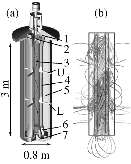
Figure 1: The Riga dynamo experiment and its eigenfield. (a) Details of the central dynamo module. 1 - Upper bending region; 2 - Propeller; 3 - Central helical flow region; 4 - Return-flow region; 5 - Outer sodium region; 6 - Guiding vanes for straightening the flow in the return flow. 7 - Lower bending region. At approximately 1/3 (L) and 2/3 (U) of the dynamo height there are four ports for various magnetic field, pressure and velocity probes. (b) Simulated structure of the magnetic eigenfield in the kinematic regime.

With view on the future utilization of the Riga dynamo experiment, here we deal with the general question whether the facility could be modified in such a way that it exhibits a more complicated saturation behaviour. One idea that comes to mind is the principle possibility to lower the critical $Rm$ by means of a parametric resonance, or swing excitation, (Rohde, Rüdiger and Elstner 1999) with a periodic flow forcing with approximately the double of eigenfrequency. We feel, however, that the comparably high frequency (around 4 Hz and larger) that would be needed for this purpose is far beyond the technical specifications of the utilized motors and their control.

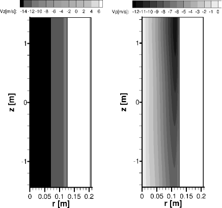
Figure 2: Assumed kinematic velocity structure in the central part of the inner tube and in the back-flow tube at a rotation rate of 2100 rpm. Axial velocity $v_{z}(r,z)$ (l.h.s) and azimuthal velocity $v_{\varphi}(r,z)$ (r.h.s.). Note the slight downward decay of $v_{\varphi}(r,z)$. Figure adopted from (Gailitis et al. 2002)

.

Another idea, namely to modify the present ratio of azimuthal velocity $v_{\varphi}$ and axial velocity $v_{z}$, is motivated by the following considerations: The Riga dynamo had been constructed in such a way that the flow helicity is maximum for a given kinetic energy (Gailitis et al. 2004) which implies the ratio of $v_{\varphi}$ to $v_{z}$ to be close to 1. Now, since the saturation mechanism relies strongly on a selective braking of $v_{\varphi}$ one could ask for the consequences if one would start with a too strong $v_{\varphi}$. Its braking would then lead to a reduced ratio $v_{\varphi}$ to $v_{z}$ which might be suspected to be even better suited for dynamo action than the original kinematic flow. In the extreme form this mechanism could lead to a sub-critical Hopf bifurcation, meaning that the velocity in the saturated state has a lower critical $Rm$ than the kinematic (unperturbed) velocity. This effect should be detectable in form of a hysteretic behaviour of self-excitation, similar to the case studied recently by Reuter et al. (2008). But even if an ”honest” sub-critical Hopf bifurcation could not be achieved, a general tendency of the system to oscillate between a weak-field and a strong-field state is still to be expected. Since such an oscillation would appear from the destabilization of the (former) steady equilibrium between Lorentz forces and inertial forces, it should be called a magneto-inertial wave, similar to the waves that have been observed in the DTS-experiment in Grenoble (Schmitt 2010).

Further, if such an oscillation with a second frequency sets in, one could also ask for the appearance of more frequencies and possibly for a transition to chaos according to the Ruelle-Takens-Newhouse scenario (Eckmann 1981).

These foregoing ideas delineate the scope of the present paper. In the second section, we will describe briefly the Riga dynamo, and present the utilized scheme for its numerical simulation. Then we will discuss two sorts of parameter variations that both start from the well-known single-frequency saturation state and end up with a chaotic regime. The paper concludes with a few remarks concerning the technical feasibility of the proposed modification.

2 The Riga dynamo and the numerical code for its simulation

An illustration of the Riga dynamo, and of its magnetic eigenfield is shown in Fig. 1. The facility consists basically of three concentric cylinders. In the innermost cylinder, the liquid sodium undergoes a downward spiral motion with optimized helicity. In the second cylinder, it flows back to the propeller region. The third cylinder serves for improving the electromagnetic boundary conditions which helps in achieving a minimum critical $Rm$. More details about the facility and the experimental campaigns can be found in (Gailitis et al. 2000, 2001, 2003, 2004, 2008). In the present configuration, self-excitation occurs approximately at a propeller rotation rate of $P=1840$ rpm when scaled appropriately to a reference temperature of 157^∘C. The shape of the magnetic eigenfield resembles a double-helix that rotates around the vertical axis with a frequency in the range of 1-2 Hz.

Figure 3: Influence of the increasing ratio of $v_{\varphi}$ and $v_{z}$ (factor $A$ compared with the present flow structure) on the time evolution. From top to bottom: A=1, 1.3, 1.7, 2.0, 2.5, 3.0. From left to right: Magnetic field energy and $B_{z}(r=0.086\mbox{ m},z=-0.39\mbox{ m})$ (first column), two-dimensional phase portrait of $B_{z}$ and $v_{\varphi}$ at $(r=0.086\mbox{ m},z=-0.39\mbox{ m})$ (second column), three-dimensional phase portrait of $B_{r}$, $B_{\varphi}$, and $B_{z}$ $(r=0.086\mbox{ m},z=-0.39\mbox{ m})$ (third column), power spectral density of $B_{z}(r=0.086\mbox{ m},z=-0.39\mbox{ m})$ (fourth column).

The numerical simulations of this paper will be carried out by means of a code that couples a solver for the induction equation

$$\frac{\partial{{\bf{B}}}}{\partial t}=\nabla\times({\bf{v}}\times{\bf{B}})+\frac{1}{\mu_{0}\sigma}\Delta{\bf{B}}\;.$$ (1)

for the azimuthal $m=1$ component of the magnetic field $\bf B$, and a simplified solver for the velocity perturbation. The solver for the induction equation is a two-dimensional finite difference scheme with a non-homogeneous grid in $r$ and $z$, that uses an Adams-Bashforth method of second order for the time integration (cf. Gailitis et al. 2004 for more details). The real geometry of the dynamo module has been slightly simplified, with all curved parts in the bending regions being replaced by rectangular ones. The unperturbed velocity in the central channel was inferred from a number of measurements at a water test facility and some extrapolations. These measurements had revealed a slight downstream decay of $v_{\varphi}$. The velocity in the back-flow channel has been considered as purely axial and constant in $r$ and $z$, with the constraint that the volume flux there is equal to the volume flux in the inner cylinder. Figure 2 shows the assumed kinematic velocity components $v_{z}(r,z)$ and $v_{\varphi}(r,z)$ both in the central channel and in the back-flow channel.

Figure 4: The three lowest dominant frequencies for increasing factor $A$. $f_{1}$ denotes the frequency of the magnetic eigenfield, $f_{2}$ is the frequency of the first magneto-inertial oscillation, $f_{3}$ is the third arising frequency. $f_{4}$ corresponds approximately to the combination $f_{1}+f_{2}-f_{3}$.

The induction equation solver has been extensively used in the optimization of the Riga dynamo experiment, and its main results (in particular concerning the growthrate and the frequency of the eigenfield) agree to a very few percent with the experimental results.

Figure 5: Same as Fig. 3, but for increasing propeller rotation rate $P$ at fixed factor $A=1.5$. From to to bottom: $P=$ 1900, 2600, 3000, 3600, 4500, 6000 rpm.

As for the saturation regime, our code tries to take into account the most important back-reaction effect within a simple one-dimensional model (see Gailitis et al. 2002, 2008). While $v_{z}$ can be assumed rather constant from top to bottom due to mass conservation, $v_{\varphi}$ can be easily braked by the Lorentz forces without any significant pressure increase. In the inviscid approximation, and considering only the $m=0$ mode of the Lorentz force, we end up with the differential equation for the Lorentz force induced perturbation $\delta v_{\varphi}(r,z)$ of the azimuthal velocity component:

$$\frac{\partial}{\partial t}\delta v_{\varphi}(r,z,t) = -\bar{v}_{z}(r,z)\frac{\partial}{\partial z}\delta v_{\varphi}(r,z,t)$$

$$+\frac{1}{\mu_{0}\rho}[(\nabla\times{\bf{B}})\times{\bf{B}}]_{\varphi}(r,z,t)\;\;.$$

In contrast to the procedure described in (Gailitis et al. 2002, 2004, 2008) which was focused exclusively on a stationary saturated regime, here we take into account the time dependence of $\delta v_{\varphi}(r,z,t)$ explicitly.

Note that Eq. 2 is solved both in the innermost channel where it describes the downward braking of $v_{\varphi}$, as well as in the back-flow channel where it describes the upward acceleration of $v_{\varphi}$. Both effects together lead to a reduction of the differential rotation and usually to a deterioration of the dynamo capability of the flow, quite in accordance with Lenz’s rule. As a technical remark, note that Eq. 2 is time-stepped independently in the innermost channel and the back-flow channel, with time-independent profiles set on two disconnection lines. The first disconnection line is in the central channel directly behind the propeller where the $v_{\varphi}(r)$ profile is set to the water-test profile (multiplied by $A$). The second disconnection line is at the bottom of the back-flow channel behind the straightening blades where $v_{\varphi}(r)$ is always set to zero.

The main result of this code, the downward accumulating braking of $v_{\varphi}$, has been shown to be in reasonable agreement with experimental data, and with the results of a much more elaborated T-RANS simulation (see Kenjeres et al. 2006, 2007), apart from the fact that the latter simulation results in an additional slight radial redistribution of $v_{z}$ that cannot be covered by our simple back-reaction model.

In the following we will use the physical units of the Riga dynamo experiment, i.e. the real geometry, velocity and conductivity with the only compromise that we will always use the conductivity $\sigma=8.56\times 10^{6}$ S/m at the reference temperature $T=157^{\circ}$C (which was used in all previous publications on the Riga dynamo). If we would dare, however, to lower the temperature to $T=102^{\circ}$C (i.e. 5^∘C above melting temperature) we would get $\sigma=10.28\times 10^{6}$ S/m, and the presently achievable propeller rotation rate of $P=2500$ rpm would than be equivalent (in terms of the magnetic Reynolds number) to 3000 rpm.

With the reference conductivity $\sigma=8.56\times 10^{6}$ S/m we obtain a diffusion time $t_{\rm diff}=\sigma\mu_{0}R^{2}_{1}=0.168$ sec if the innermost radius $R_{1}=0.125$ is used, or 1.72 sec if we take the outer radius $R_{3}=0.4$ m. The integration time for our runs was set to 6.25 sec, which in some cases is not completely sufficient for all relaxations to be finalized.

3 Numerical results

In this section we present the numerical results for two types of parameter variations. The first variation starts from a state that corresponds approximately to the maximum achievable $Rm$ number of the present Riga dynamo set-up, from where we artificially scale up $v_{\varphi}$ by a factor $A$, keeping $v_{z}$ fixed. In the second variation we scale-up the magnetic Reynolds number (in terms of the propeller rotation rate $P$) while keeping the ratio of $v_{\varphi}$ and $v_{z}$ fixed at $A=1.5$.

Figure 6: Same as Fig. 4, but for increasing P at fixed $A=1.5$.

The variation documented in Fig. 3 starts from a given propeller rotation rate $P=3000$ rpm with the present ratio of $v_{\varphi}$ to $v_{z}$ (corresponding to $A=1$). Keeping the profile of $v_{z}$ fixed, we artificially increase then $v_{\varphi}$. The rows from top to bottom in Fig. 3 correspond to increasing factors $A=$1.0, 1.3, 1.7, 2.0, 2.5, 3.0. For each row, the first column shows the time evolution of the magnetic field component $B_{z}$ at radius $r=0.086$ m and axial position $z=-0.39$ m (with respect to the mid-height of the dynamo) and of the total magnetic field energy. The second column depicts the two-dimensional phase portrait of $B_{z}$ and $v_{\varphi}$ at the same position $(r=0.086\mbox{ m},z=-0.39\mbox{ m})$. The third column shows a three-dimensional phase portrait in the three magnetic field components $B_{r}$, $B_{\varphi}$, and $B_{z}$ at the same position. Finally, the fourth column gives the power spectral density of $B_{z}(r=0.086\mbox{ m},z=-0.39\mbox{ m})$

For $A=1.0$ we obtain the well-known single-frequency oscillation (resulting from the rotating magnetic eigenfield) with a frequency $f_{1}=2.13$ Hz, which translates into a (more or less) horizontal line in the $B_{z}$-$v_{\varphi}$ plot and a circle in the $B_{r}$-$B_{\varphi}$-$B_{z}$ phase portrait. For $A=1.3$, a second frequency $f_{2}=1.71$ Hz comes into play, which is a signature of an arising magneto-inertial oscillation. Accordingly, the three-dimensional phase portrait shows a torus structure. Around $A=2.0$ a third frequency arises. For $A=2.5$ and $A=3.0$ we observe then a irregular, probably chaotic behaviour, which manifests itself in the phase portraits and the smeared out PSD.

In Fig. 4 we have compiled the three lowest peaks $f_{1}$, $f_{2}$, and $f_{3}$ of the frequency spectrum. We have also indicated a fourth frequency, $f_{4}$, which seems to agree with the combination $f_{1}+f_{2}-f_{3}$. It is important to note that these spectral properties have still a preliminary character because the simulation time comprises only a few oscillations. Anyway, there is some evidence that the appearance of the third frequency ”rings in” the on-set of irregular behaviour by destabilizing the two-torus made up by the first two frequencies $f_{1}$ and $f_{2}$.

A second parameter variation, for which the value $A$ is now fixed to 1.5, while the propeller rotation rate $P$ is increased, is illustrated in Figs. 5 and 6. The rows from top to bottom in Fig. 4 correspond now to the axial propeller rotation rates $P=$1900, 2600, 3000, 3600, 4500, 5000, 6000 rpm.

The main features are quite similar as in the former sequence, apart from the fact that the ratio $f_{1}/f_{2}\sim 2$ stays rather constant within the wide range of $P=1900...4000$ rpm, a fact that points to a phenomenon called ”mode locking”. This is best visible in the appearance of a rather sharp ratio $f_{1}/f_{2}=2.0$ for $P=3600$ rpm (fourth row) in Fig. 5).

Figures 7 and 8 illustrate the character of the magneto-inertial wave for $A=1.5$ and two selected values $P=$ 3600 and 6000 rpm, respectively. In each case, the upper panel shows $v_{\varphi}(r=0.086\mbox{ m},z,t)$, and the lower panel shows $B_{r}(r=0.086\mbox{ m},z,t)$. While the case $P=3600$ rpm shows a frequency-locked wave, the case $P=6000$ is already much more irregular.

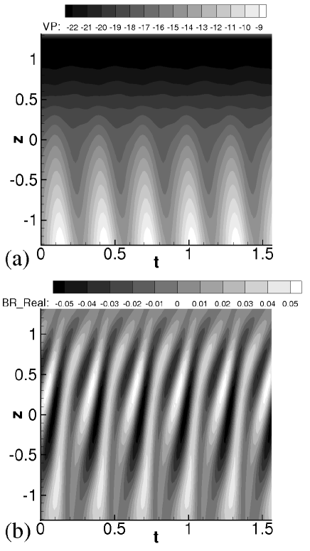
Figure 7: $t-z$-dependence of $v_{\varphi}(r=0.086\mbox{ m},z,t)$ (a) and $B_{r}(r=0.086\mbox{ m},z,t)$ (b) for $A=1.5$ and $P=3600$ rpm. The unit of $v_{\varphi}$ is m/s, the unit of $B_{r}$ is Tesla.

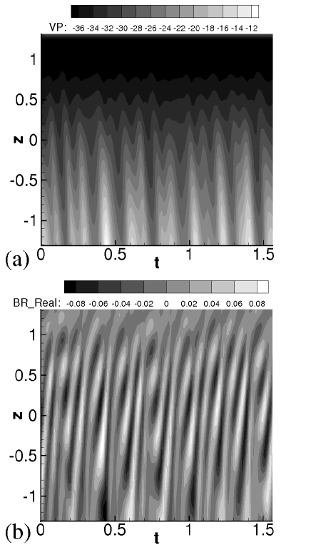
Figure 8: Same as Fig. 7, but for $A=1.5$ and $P=6000$ rpm.

4 Conclusions

Presently, the maximum $Rm$ in the Riga dynamo experiment can be achieved with a propeller rotation rate of 2500 rpm and a temperature of around 102^∘C, which is roughly equivalent to a propeller rotation rate of 3000 rpm at a reference temperature of 157^∘C. Starting from this realistic set-up that leads to a single-frequency saturated state, we have studied hypothetical modifications of the sodium flow in which the present ratio of $v_{\varphi}$ and $v_{z}$ is scaled-up by a factor $A$. Beginning approximately at $A=1.3$ we observe the appearance of a magnetic field energy oscillation with a frequency $f_{2}$ that is in the order of one half of the eigenfrequency $f_{1}$ of the saturated dynamo.

We hypothesize that this new oscillation with frequency $f_{2}$ is basically a magneto-inertial wave that traces back to the fact that the steady equilibrium between Lorentz and inertial forces (that is responsible for the saturation) becomes unstable if the ratio of $v_{\varphi}$ and $v_{z}$ velocity is larger than the optimum value. This allows the system to oscillate between a weak field and a strong field limit.

For increasing factors $A$ we observe further the appearance of a third frequency $f_{3}$ and then the transition to a rather irregular, probably a chaotic state. Similar transitions are observed when increasing the propeller rotation rate $P$ while holding the factor $A$ fixed at a value of 1.5. An interesting feature of this latter sequence is the appearance of a sort of frequency locking (characterized $f_{1}/f_{2}=2$ ) for a rather wide range of $2600<P<3600$.

The observed behaviour resembles the Ruelle-Takens-Newhouse scenario of the transition to chaos (see Eckmann 1981). We have to point out, though, the preliminary character of our study, both with respect to limited integration time as well as to the fact that a detailed study of the space and time resolution is still missing.

What remains to be checked further is the possible existence of a sub-critical Hopf-bifurcation.

The delineated mechanism to obtain energy oscillations in the saturated state, and even the sketched route to chaos, seems to be in the range of technical feasibility if we assume approximately a doubling of the motor power and an increase of the ratio of azimuthal to axial velocity by means of an appropriate propeller and guiding blade design.

- [1] Eckmann, J.-P.: 1981, Rev. Mod. Phys. 53, 643
- [2] Gailitis, A., Freibergs, Ya.: 1976, Magnetohydrodynamics 12, 127
- [3] Gailitis, A., Freibergs, Ya.: 1980, Magnetohydrodynamics 16, 116
- [4] Gailitis, A., Lielausis, O., Dement’ev, S., et al.: 2000, Phys. Rev. Lett. 84, 4365
- [5] Gailitis, A., Lielausis, O., Platacis, O., et al.: 2001, Phys. Rev. Lett. 86, 3024
- [6] Gailitis, A., Lielausis, O., Platacis, E., Gerbeth, G, Stefani, F.: 2002, Magnetohydrodynamics 38, 15
- [7] Gailitis, A., Lielausis, O., Platacis, E., Gerbeth, G, Stefani, F.: 2003, Surv. Geophys. 24, 247
- [8] Gailitis, A., Lielausis, O., Platacis, E., Gerbeth, G, Stefani, F.: 2004, Phys. Plasmas 11, 2838
- [9] Gailitis, A., Gerbeth, G., Gundrum, T., Lielausis, O., Platacis, E., Stefani, F.: 2008, Compt. Rend. Phys. 9, 721
- [10] S. Kenjereš, S., Hanjalić, K., Renaudier, S. Stefani, F., Gerbeth, G., Gailitis, A.: 2006, Phys. Plasmas 13, 122308.
- [11] Kenjereš, S., Hanjalić, K.: 2007, Phys. Rev Lett. 98,104501.
- [12] Ponomaranko, Yu.B.: 1973, J. Appl. Mech. Tech. Phys. 14, 775
- [13] Ravelet, F., Berhanu, M., Monchaux, R., et al.: 2008, Phys. Rev. Lett. 101, 074501
- [14] Rohde, R., Rüdiger, R., Elstner, D.: 1999, Astron. Astrophys. 347, 860
- [15] Reuter, K., Jenko, F., Forest, C.B.: 2009, New J. Phys. 11, 013027
- [16] Schmitt, D.: 2010, Geophys. Astrophys. Fluid Dyn. 104, 135
- [17] Stefani, Gailitis, A., Gerbeth, G.: 2008, ZAMM 88, 930