Free probability, Planar algebras, Subfactors and Random Matrices.

Abstract

To a planar algebra $\mathcal{P}$ in the sense of Jones we associate a natural non-commutative ring, which can be viewed as the ring of non-commutative polynomials in several indeterminates, invariant under a symmetry encoded by $\mathcal{P}$. We show that this ring carries a natural structure of a non-commutative probability space. Non-commutative laws on this space turn out to describe random matrix ensembles possessing special symmetries. As application, we give a canonical construction of a subfactor and its symmetric enveloping algebra associated to a given planar algebra $\mathcal{P}$. This talk is based on joint work with A. Guionnet and V. Jones.

rimary: 46L37, 46L54; Secondary 15A52.

1 Introduction.

The aim of this paper is to explore the appearance of planar algebra structure in three areas of mathematics: subfactor theory; free probability theory; and random matrices.

Jones’ subfactor theory has lead to a revolution in understanding what may be termed “quantum symmetry”. The standard invariant of a subfactor — the so-called lattice of higher relative commutants, or “$\lambda$-lattice” [Pop95, GHJ89] is a remarkable mathematical object, which can represent a very general type of symmetry. For example, a subfactor inclusion (and so its standard invariant) can be associated to a Lie group representation. In this case, the vector spaces that make up the standard invariant are the spaces of intertwiners between tensor powers of that representation. Thus the standard invariant of such a subfactor can be used to encode the representation theory of a Lie group, and thus symmetries associated with Lie group actions.

In his groundbreaking paper [Jon99, Jon01] Jones (building on an earlier algebraic axiomatization of standard invariants by Popa [Pop95]) showed that there is a striking way to characterize standard invariants of subfactors: these are exactly planar algebras (see §3.4 below for a definition). Very roughly, one can think of a planar algebra as a sequence of vector spaces consisting of vectors invariant under some “quantum symmetry”, together with very general ways (dictated by planar diagrams) of producing new invariant vectors from existing vectors. The planar algebra thus encodes the underlying symmetry. In the context of the present paper, we shall use the terms “quantum symmetry” and “planar algebra” interchangeably.

Curiously, planar diagrams also occur in random matrix theory. Certain random multi-matrix ensembles (see 4.7 below) are asymptotically described by combinatorics involving counting planar maps (these objects are very much like planar diagrams appearing in the definition of planar algebras). This fact has been discovered and extensively used by physicists, starting from the works of ’t Hooft, Brezin, Iszykson, Parisi, Zuber and others (see e.g. [tH74, BIPZ78]). A rigorous proof of convergence was obtained by Guionnet and Maurel Segala (see [Gui06, GMS06] and references therein) and Ercolani and McLaughlin [EM03].

Finally, turning to Voiculescu’s free probability theory [VDN92], it was shown by Speicher [Spe94] and others that many important free probability laws (such as the semicircle law, the free Poisson law and so on) have combinatorial descriptions involving counting planar objects (such as non-crossing partitions, which are also very closely related to planar diagrams).

Thus one is faced with two natural questions. First, why do these planar structures appear in these three areas? And second, how can these similarities be exploited?

Concerning the first question, we do not know a fully satisfactory answer. However, if one grants that planar structure is necessary to describe “quantum symmetries” (i.e., subfactors), then one is able to find explanations for appearances of planar structure in free probability theory and random matrices. We show that one has a natural notion of a non-commutative probability law having a quantum symmetry — this law is given by a trace on a ring naturally associated to a planar algebra. Mathematically, this is accomplished by a “change of rings” procedure, where we replace the ring of non-commutative polynomials in $K$ variables with a certain canonical ring associated to a given planar algebra (see §3.9). This “change of rings” is analogous to the passage from some probability space $\Omega$ to the quotient space $\Omega/G$ in the case that the laws of some family of random variables are invariant under the action of a group $G$.

Also, we show how to construct random matrix ensembles, which asymptotically give rise to a non-commutative law with a given quantum symmetry.

This means that any time one considers a natural equation in free probability theory, or a natural equation giving the asymptotics of a random matrix ensemble, this equation must make sense not only as an equation involving polynomials in $K$ non-commuting indeterminates, but also arbitrary planar algebra elements. Thus the equation (and so its solutions) must have a natural planar structure.

Concerning the second question, we give a number of applications of our techniques. One such application is a version of the ground-breaking theorem of Popa [Pop95, PS03] which states that every planar algebra $\mathcal{P}$ arises from a subfactor $N\subset M$ with $N,M$ isomorphic to free group factors. It turns out that both $N$ and $M$ can in fact be chosen to be natural non-commutative probability spaces “in the presence of the symmetry $\mathcal{P}$”. On the random matrix side, our approach gives a mathematical framework to formulate the work of a number of physics authors [EZJ92, Kos89, ZJ03] on the so-called $O(n)$ matrix model. In fact, using our techniques one can make rigorous sense of the $O(n)$ matrix model for $n\in\{2\cos\frac{\pi}{n}:n\geq 3\}\cup[2,+\infty)$ (non-integer values of $n$ are used in the physics literature).

The remainder of the paper is organized as follows. We first discuss some basic notions from free probability theory and subfactors. Next, we discuss a notion of a non-commutative probability law having a symmetry encoded by a planar algebra $\mathcal{P}$ and present some applications to subfactor theory. Finally, we show that one can construct random matrix ensembles that model certain non-commutative laws with a given planar algebra symmetry $\mathcal{P}$, and explain connections with a class of random matrix ensembles used in the physics literature, and derive some random matrix consequences.

This paper is based on the joint work with A. Guionnet and V.F.R. Jones [GJS08, GJS09].

2 Background and basic notions: Free probability and non-commutative probability spaces.

2.1 Non-commutative probability spaces

Recall (see for example [VDN92]) that an algebraic non-commutative probability space $(A,1_{A},\tau)$ consists of an algebra $A$ with unit $1_{A}$ and a unital linear functional $\tau:A\to\mathbb{C}$. We often make the assumption that $A$ is a $*$-algebra and $\tau$ is a trace, i.e., $\tau(ab)=\tau(ba)$ for all $a,b\in A$. Elements of $A$ are called non-commutative random variables. Here are a few examples:

Example 2.2.

(a) If $(\mathfrak{X},\mu)$ is a measure space and $\mu$ is a probability measure, then $(A=L^{\infty}(\mathfrak{X},\mu),1_{A},f\stackrel{{\scriptstyle\tau}}{{\to}}\int fd\mu)$ is a non-commutative probability space.
(b) For any $N$, the algebra of $N\times N$ matrices $(A=M_{N\times N}(\mathbb{C}),1_{A}=\textrm{Id},\tau=\frac{1}{N}Tr)$ is a non-commutative probability space.
(c) Consider $A=M_{N\times N}(L^{\infty,-}(\mathfrak{X},\mu))$, with $(\mathfrak{X},\mu)$ as in (a). Thus elements of $A$ are random matrices. Then $(A,1_{A},\mathbb{E}(\frac{1}{N}Tr(\cdot)))$ is a non-commutative probability space.

Note that in all of these examples, $\tau$ is a trace: $\tau(xy)=\tau(yx)$.

In order to be able to do analysis on non-commutative probability spaces we make the assumption that the algebra $(A,1_{A},\tau)$ is represented (by bounded or unbounded operators) on a Hilbert space $H$ by a faithful unital representation $\pi$, so that $\tau(a)=\langle\Omega,\pi(a)\Omega\rangle$ for some fixed vector $\Omega\in H$.

Elements of non-commutative probability spaces are called non-commutative random variables.

2.3 Non-commutative laws

Given $K=1,2,\dots$ classical real random variables $X_{1},\dots,X_{K}$, which we can think of as an $\mathbb{R}^{K}$-valued function $X$ on some probability space $(\mathfrak{X},\mu)$, their joint law is defined to be the push-forward by $\tau=X_{*}\mu$ of $\mu$ to a probability measure on $\mathbb{R}^{K}$. If $\mu$ has finite moments, we obtain a linear functional on the algebra of polynomials on $\mathbb{R}^{K}$.

By analogy, given non-commutative random variables $X_{1},\dots,X_{K}\in A$, their non-commutative law $\tau_{X_{1},\dots,X_{K}}$ is the linear function on the algebra of all non-commutative polynomials in $K$ indeterminates $\mathbb{C}[t_{1},\dots,t_{K}]$ obtained by composing $\tau$ with the canonical map sending $t_{j}$ to $X_{j}$. In other words

$$\tau_{X_{1},\dots,X_{K}}(P(t_{1},\dots,t_{K}))=\tau(P(X_{1},\dots,X_{K}))$$

for any non-commutative polynomial $P$.

If $K=1$, non-commutative laws are the same as commutative laws, modulo identification of measures with linear functionals they induce on polynomials by integration. For example, in the case of a single self-adjoint matrix $Y\in(M_{N\times N},\frac{1}{N}Tr)$, its non-commutative law corresponds to integration against the measure $\mu_{Y}=\frac{1}{N}\sum\delta_{\lambda_{j}}$, where $\lambda_{1},\dots,\lambda_{N}$ are the eigenvalues of $Y$. If $Y$ is a random matrix, its non-commutative law captures the expected value of the random spectral measures associated to $Y$, $\mathbb{E}(\mu_{Y})$.

The classical notion of independence of random variables can be reformulated algebraically by stating that $(X_{1},\dots,X_{K})$ is independent from $(X_{K+1},\dots,X_{K+L})$ in a non-commutative probability space $(A,\tau)$ if the law of $(X_{1},\dots,X_{K+L})\in(A,\tau)$ is the same as that of the variables

$$(\alpha_{1}(X_{1}),\dots,\alpha_{1}(X_{K}),\alpha_{2}(X_{K+1}),\dots,\alpha_{2}(X_{K+L}))\in(A\otimes A,\tau\otimes\tau).$$

Here $\alpha_{1}(X)=X\otimes 1$, $\alpha_{2}(X)=1\otimes X$ are two natural embeddings of $A$ into $A\otimes A$.

Voiculescu developed his free probability theory (see e.g. [VDN92]) around another notion of independence, free independence. For this notion, we say that $(X_{1},\dots,X_{K})$ is freely independent from $(X_{K+1},\dots,X_{K+L})$ in a non-commutative probability space $(A,\tau)$ if the law of $(X_{1},\dots,X_{K+L})\in(A,\tau)$ is the same as that of the variables

$$(\alpha_{1}(X_{1}),\dots,\alpha_{1}(X_{K}),\alpha_{2}(X_{K+1}),\dots,\alpha_{2}(X_{K+L}))\in(A*A,\tau*\tau),$$

where $*$ denotes the free product [Voi85, VDN92], and $\alpha_{1}$, $\alpha_{2}$ are the natural embeddings of $A$ into $A*A$ (into the first and second copy, respectively).

If $\tau$ is a non-commutative law satisfying positivity and boundedness requirements, the GNS construction yields a representation of $\mathbb{C}[t_{1},\dots,t_{K}]$ on $L^{2}(\tau)$ and thus generates a von Neumann algebra $W^{*}(\tau)$. The non-commutative case here differs significantly from the commutative case. In the commutative case, $W^{*}(\tau)=L^{\infty}(\mathfrak{X})$, and, notably, all measure spaces $\mathfrak{X}$ are isomorphic (at least for laws $\tau$ which are non-atomic). In the non-commutative case, the von Neumann algebras $W^{*}(\tau)$ are much more diverse, and it is in general a very difficult and challenging question to decide, for two laws $\tau,\tau^{\prime}$, when $W^{*}(\tau)\cong W^{*}(\tau^{\prime})$, or to somehow identify the isomorphism class of $W^{*}(\tau)$.

3 Symmetries: Subfactors, Planar algebras, and non-commutative laws

3.1 Non-commutative laws with quantum symmetry

Consider a complex-valued classical random variable $Z$; thus we actually have a pair of random variables $Z,\bar{Z}$, whose joint law is described by a probability measure $\mu$ on $\mathbb{C}=\mathbb{R}^{2}$: for any function of two variables $f(x,y)$, we are interested in the value

$$\iint f(z,\bar{z})d\mu(z,\bar{z}).$$

In this way, the law of $(Z,\bar{Z})$ is a functional on the space of functions on $(-\infty,\infty)\times(-\infty,\infty)$.

Assume that we know that the law of $(Z,\bar{Z})$ is invariant under rotations: $(Z,\bar{Z})\sim(wZ,\bar{w}\bar{Z})$ for any $w\in\mathbb{C}$, $|w|=1$. Then the joint law of $(Z,\bar{Z})$ is completely determined by its “radial part”, the integrals of the form

$$\int g(|z|)d\mu(z,\bar{z}),$$

and thus defines a linear functional on the space of rotation-invariant functions, i.e., effectively on the space of functions on $[0,+\infty)=\mathbb{C}^{2}/\mbox{rotation}$.

Thus the presence of a symmetry dictates that we use a different probability space. Our aim is to extend this observation to the non-commutative setting, allowing the most general notions of symmetry possible.

We defined a non-commutative probability law to be a linear functional $\tau$ defined on the algebra $A=\mathbb{C}[X_{1},\dots,X_{K}]$ of non-commutative polynomials in $K$ variables. If symmetries are present, this choice of the algebra $A$ may not be suitable. In this case the algebra $A$ (the non-commutative analog of the ring of polynomials on $\mathbb{R}^{K}$) must be replaced by the analog of the ring of functions on a different algebraic variety. For instance, one may be interested in $*$-probability spaces, i.e., we want to have an algebra $A$ that has a non-trivial adjoint operation (involution). This can be accomplished by considering the algebra $B=\mathbb{C}[X_{1},\dots,X_{K},X_{1}^{*},\dots,X_{K}^{*}]$ and defining $X_{j}^{*}$ to be the adjoint of $X_{j}$. An even more interesting situation is the case that our algebra $B$ has a natural symmetry. For example, we may consider the action of the unitary group $U(K)$ on $B$ given on the generators by

$$U\cdot X_{k}=\sum U_{ik}X_{i},\qquad U\cdot X_{k}^{*}=\sum\overline{U_{ik}}X_{i}^{*},\qquad\quad U=(U_{ij}).$$ (3.1.1)

In this case we may only be interested in a part of $B$, the algebra $B^{U(K)}$ consisting of $U(K)$-invariant elements. One can easily see that $B^{U(K)}$ is not even a finitely-generated algebra, but it is the natural non-commutative probability space on which to define $U(K)$-invariant laws.

More generally, in this paper we will be interested in non-commutative laws defined on a class of “symmetry algebras”, which are the analogs of algebras such as $B^{U(K)}$ above for more general symmetries (including actions of quantum groups).

As is well-known, subfactor theory of Jones provides a framework for considering such very general symmetries. To formalize our notion of a “non-commutative probability law with a quantum symmetry”, we shall first review Jones’ notion of planar algebras [Jon99, Jon01].

3.2 The standard invariant of a subfactor: spaces of intertwiners

Planar algebras [Jon99, Jon01] were introduced by Jones in his study of invariants of subfactors of II₁ factors.

Let $M_{0}\subset M_{1}$ be an inclusion of II₁ factors of finite Jones’ index [Jon83, GHJ89]. Then $M_{1}$ can be regarded as a bimodule over $M_{0}$ by using the left and right multiplication action of $M_{0}$ on $M_{1}$. Using the operation of the relative tensor product of bimodules (see e.g. [Con, Pop86, Con94, Bis97]) one can construct other $M_{0},M_{0}$-bimodules by considering tensor powers

$$M_{k}=\underbrace{M_{1}\otimes_{M_{0}}\otimes\cdots\otimes_{M_{0}}M_{1}}_{k}.$$

One can then consider the intertwiner spaces

$$A_{ij}=\operatorname{Hom}_{M_{0},M_{0}}(M_{i},M_{j})$$

consisting of all homomorphisms from $M_{i}$ to $M_{j}$, which are linear for both the left and the right action of $M_{0}$. Because the index of $M_{0}\subset M_{1}$ is finite, these spaces turn out to be finite-dimensional. The system of intertwiner spaces $A_{ij}$ has more structure than the algebra structure of the individual $A_{ij}$’s. For example, having an intertwiner $T:M_{i}\to M_{j}$ one can also construct an “induced representation” intertwiner $T\otimes 1:M_{i+1}\to M_{j+1}$. More generally, one can restrict intertwiners, take their tensor products, etc., thus providing many operations involving elements of the various $A_{ij}$’s.

The following example explains how classical representation theory of a Lie group can be viewed in subfactor terms. Similar examples exist also in the case of quantum group representations:

Example 3.3.

Let $G$ be a Lie group and $V$ be an irreducible representation of $G$, and denote by $V^{op}$ the representation on the dual of $V$. Let $M$ be a II₁ factor carrying an action of $G$ satisfying a technical condition of being properly outer (such an action always exists with $M$ a hyperfinite II₁ factor or a free group factor). Consider the “Wassermann-type” inclusion

$$M_{0}=M^{G}\subset(M\otimes End(V))^{G}=M_{1}.$$

Here $N^{G}$ denotes the fixed points algebra for an action of $G$ on $N$, and $G$ acts on $End(V)$ by conjugation. Then

$$\operatorname{Hom}_{M_{0},M_{0}}(M_{k}) =\operatorname{Hom}_{G}(\underbrace{V\otimes V^{op}\otimes\cdots\otimes V\otimes V^{op}}_{k})$$

is the space of all $G$-invariant linear maps on $(V\otimes V^{op})^{\otimes k}$.

The main theorem of Jones [Jon99, Jon01] is that there is a beautiful abstract characterization of systems of intertwiner spaces associated to a subfactor (also called “standard invariants”, “$\lambda$-lattices”, systems of higher-relative commutants): such systems are exactly the planar algebras. His proof relied on an earlier axiomatization of $\lambda$-lattices by Popa [Pop95].

3.4 Planar algebras

To state the definition of a planar algebra, let us introduce the notion of a planar tangle $T$ with $r$ input disks or sizes $k_{1},\dots,k_{r}$ and output disk of size $k$ (we’ll write $\mathcal{T}(k_{1},\dots,k_{r};k)$ for the set of such tangles). Such a tangle is given by drawing (up to isotopy on the plane) $r$ “input” disks $(D_{j}:j=1,\dots,r)$ inside the “output” disk $D$. Each disk $D_{l}$ has $2k_{l}$ points marked on its boundary (one of which is marked as the “first” point). The output disk $D$ has $2k$ points marked on its boundary, one of which is marked “first”. Furthermore, all marked boundary points are connected to other marked points by non-crossing paths.

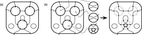
Figure 1: Planar tangles; composing planar tangles.

Figure 1(a) shows an example of a planar tangle in $\mathcal{T}(3,3,2;3)$; the first point on each interior disk is labeled by a $*$. Note that tangles may contain loops which are not connected to any interior disks.

Tangles can be composed by gluing the output disk of one tangle inside an input disk of another tangle in a way that aligns points marked “first” and preserves the orientation of boundaries (see Figure 1(b), which illustrates the composition of a tangle in $\mathcal{T}(3,3,2;3)$ with three tangles, from $\mathcal{T}(4;6)$, $\mathcal{T}(;4)$ and $\mathcal{T}(;6)$). (This is only possible if disks are of matching sizes).

Definition 3.5.

Let $(P_{k}:k=0,1,2,\dots)$ be a collection of vector spaces. We say that $(P_{k})_{k\geq 0}$ forms a planar algebra if any planar tangle $T\in\mathcal{T}(k_{1},\dots,k_{r};k)$ gives rise to a multi-linear operation $Op(T):P_{k_{1}}\otimes\cdots\otimes P_{k_{r}}\to P_{k}$ in such a way that the assignment $T\to Op(T)$ is natural with respect to composition of tangles and of multilinear maps.

Very roughly, one should think of the spaces $P_{k}$ as the space of “intertwiners” of degree $2k$ for some quantum symmetry (see §3.6.1 below). The various operations $Op(T)$ correspond to the various ways of combining such intertwiners to form new intertwiners.

We also often make the assumption that the space $P_{0}$ is one-dimensional and all $P_{k}$ are finite-dimensional. In particular, a tangle $T$ with no input disks and one output disk with zero marked points and no paths inside gives rise to a basis element of $P_{0}$, which we’ll denote by $\emptyset$. If we instead consider a tangle $T^{\prime}$ with no input disks, one output disk with no marked points, and a simple closed loop inside of the output disk, then $T^{\prime}$ produces an element $\delta\emptyset$ in $P_{0}$ (where $\delta$ is some fixed number). Furthermore, it follows from naturality of composition of tangles that if some tangle $T$ is obtained from a tangle $T^{\prime}$ by removing a closed loop, then $Op(T)=\delta Op(T^{\prime})$.

The tangle in Figure 2(a) gives rise to a bilinear form on each $A_{k}$, which we assume to be non-negative definite. We endow each $P_{k}$ with an involution compatible with the action of orientation-preserving planar maps on tangles. Finally, we assume a spherical symmetry, so that we consider tangles up to isotopy on the sphere (and not just the plane).

A planar algebra satisfying these additional requirements is called a subfactor planar algebra with parameter $\delta$. It is a famous result of Jones [Jon83] that $\delta\in\{2\cos\frac{\pi}{n}:n\geq 3\}\cup[2,+\infty)$, and all of these values can occur.

3.6 Examples of planar algebras

Planar algebras can be thought of as families of linear spaces consisting of vectors “obeying a symmetry”, where the word symmetry is taken in a very generalized sense (such “symmetries” include group actions as well as quantum group actions). We consider a few examples:

3.6.1 Planar algebras of polynomials

Let $X_{1},\dots,X_{K},X_{1}^{*},\dots,X_{K}^{*}$ be indeterminates, and denote by $A$ the algebra spanned by alternating monomials of the form $X_{i_{1}}X_{j_{1}}^{*}\cdots X_{i_{k}}X_{j_{k}}^{*}$. Let $P_{k}$ be the linear subspace of $A$ consisting of all elements that have degree $2k$. We claim that $\mathcal{P}=(P_{k})_{k\geq 0}$ is a planar algebra if endowed with the following structure. Given a monomial $W=X_{i_{1}}X_{j_{1}}^{*}\cdots X_{i_{k}}X_{j_{k}}^{*}\in P_{k}$, associate to it the labeled disk $D(W)$ whose $2k$ boundary points are labeled (clockwise, from the “first” point) by the $2k$-tuple $(i_{1},j_{1},i_{2},j_{2},\dots,i_{k},j_{k})$. Now given a planar tangle $T\in\mathcal{T}(k_{1},\dots,k_{r};k)$ and monomials $W_{1},\dots,W_{r}$ of appropriate degrees, we define

$$Op(T)(W_{1},\dots,W_{r})=\sum_{W}C_{W}W.$$

Here the sum is over all monomials $W\in A_{k}$ and $C_{W}$ are integers obtained as follows. Glue the disks $D(W_{j})$ into the input disks of $T$ and then the output disk of $T$ into $D(W)$. We obtain a collection of disks, whose marked boundary points are connected by curves. Then $C_{W}$ is the total number of ways to assign integers from $\{1,\dots,K\}$ to these curves, so that each curve has the same label as its endpoints. ($C_{W}=0$ if no such assignment exists).

In this case, $\mathcal{P}$ is actually a subfactor planar algebra with parameter $\delta=K$ (the number of ways to assign an integer from $\{1,\dots,K\}$ to a closed loop). The corresponding subfactor inclusion is rather trivial: it corresponds to the $K\times K$ matrix inclusion $M_{0}=M\subset M\otimes M_{K\times K}(\mathbb{C})=M_{1}$, for any II₁ factor $M$.

Consider the action of the unitary group $U(K)$ on each $P_{k}$ defined by (3.1.1). In other words, we identify $P_{k}$ with the $k$-th tensor power of $\mathbb{C}^{K}\otimes\overline{\mathbb{C}^{K}}=\operatorname{End}(\mathbb{C}^{K})$, where $\mathbb{C}^{K}$ is the basic representation of $U(K)$. Then the linear subspaces $P_{k}^{U(K)}$ consisting of vectors fixed by the $U(K)$ action turn out to form a planar algebra $\mathcal{P}^{U(K)}$ (taken with the restriction of the planar algebra structure of $\mathcal{P}$). The associated subfactor has the form

$$M^{U(K)}\subset(M\otimes\operatorname{End}(\mathbb{C}^{K}))^{U(K)}.$$

3.6.2 The Temperley-Lieb planar algebra

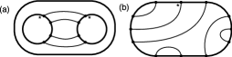
Figure 2: Canonical bilinear form; Temperley Lieb diagrams.

Let $TL_{k}$ be the linear space spanned by tangles $T\in\mathcal{T}(;k)$ with no internal disks and $2k$ points on the outer disk. Such tangles are called Temperley-Lieb diagrams (see Figure 2(b)). Then $TL=(TL_{k})_{k\geq 0}$ is a planar algebra in the following natural way. Given any tangle $T\in\mathcal{T}(k_{1},\dots,k_{r};k)$ and Temperley-Lieb diagrams $T_{1},\dots,T_{r}$ , $Op(T)(T_{1},\dots,T_{r})$ is defined to be the result of gluing the diagrams $T_{1},\dots,T_{r}$ into the input disks of $T$, provided that we agree that closed loops contribute a multiplicative factor of $\delta$. $TL$ is actually a subfactor planar algebra when $\delta$ is in the set of allowed index values $\{2\cos\frac{\pi}{n}:n\geq 3\}\cup[2,+\infty)$.

It should be noted that any planar algebra $\mathcal{P}$ contains a homomorphic image of $TL$; indeed, $TL$ elements arise as $Op(T)$ when $T\in\mathcal{T}(;k)$.

3.7 Algebras and non-commutative probability spaces arising from planar algebras

A planar algebra $\mathcal{P}=(P_{k})_{k\geq 0}$ has, by definition, a large variety of mutli-linear operations. We shall single out the following bilinear operations $\wedge_{k}$, each of which is an associative multiplication on $\oplus_{n\geq k}P_{k}$. The operation $\wedge_{k}$ takes $P_{k+n}\times P_{k+m}\to P_{k+m+n}$ and is given by the following tangle (here $k=2$, $n=1$ and $m=2$):

3.7.1 The product $\wedge_{0}$

Perhaps the easiest way to see the importance of these operations is to realize that in the case of planar algebra of polynomials (see §3.6.1) the multiplication $\wedge_{0}$ is just the ordinary multiplication of polynomials.

Thus if we think of $\oplus_{k\geq 0}P_{k}$ as a linear space consisting of vectors which are invariant under some “quantum symmetry”, the product $\wedge_{0}$ is a kind of tensor product of these invariants, and thus $(\mathcal{P},\wedge_{0})$ has the natural interpretation of the algebra of “invariant polynomials”.

3.7.2 The higher products $\wedge_{k}$

In the case of the polynomial algebra (§3.6.1), the product $\wedge_{k}$ corresponds to the product on the algebra of differential operators of degree $k$. Let us consider such operators of the form (for simplicity, if $k$ is even)

$$X_{i_{1}}X_{j_{1}}^{*}\cdots X_{i_{k/2}}X_{j_{k/2}}^{*}X_{t_{1}}X_{s_{1}}^{*}\cdots X_{t_{n}}X_{s_{n}}^{*}\partial_{X_{i_{k/2+1}}}\partial_{X_{j_{k/2+1}}^{*}}\cdots\partial_{X_{i_{k}}}\partial_{X_{j_{k}}^{*}}\in P_{k+n}.$$

Such expressions can be multiplied using the convention that $\partial_{X_{s}^{a}}X_{t}^{b}=\delta_{a\neq b}\delta_{s=t}1$, where $a,b\in\{\ ,*\}$. This is exactly the multiplication $\wedge_{k}$.

Note that the map $\mathcal{E}_{k}$ given by the tangle in Figure (3)(c) defines a natural map from $(\mathcal{P},\wedge_{k})$ to $(\mathcal{P},\wedge_{0})$.

Definition 3.8.

A planar algebra law associated to a planar algebra $\mathcal{P}$ is a linear functional $\tau$ on the algebra $(\mathcal{P},\wedge_{0})$, so that $\tau\circ\mathcal{E}_{k}$ is a trace on $(\mathcal{P},\wedge_{0})$ for any $k\geq 0$.

Since $P_{k}$ can be thought of as the space of vectors with a “quantum symmetry encoded by $\mathcal{P}$”, a planar algebra law is a law having this “quantum symmetry”.

3.9 The Voiculescu trace on $(\mathcal{P},\wedge_{0})$

Any planar algebra probability space comes with a natural trace $\tau=\tau_{TL}$ given by the tangle in Figure (3)(a).

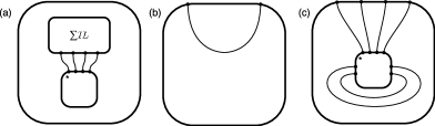
Figure 3: (a) The Voiculescu trace; here $\sum TL$ stands for the sum of all $TL$ elements with the appropriate number of strings. (b) The element $\cup$. (c) The map $\mathcal{E}_{k}$ (here $k=2$).

Lemma 3.10.

[GJS08] (Non-commutative analog of the $\chi$-squared distribution). Consider the element $\cup\in TL$ described in Figure (3)(b). Then law of $\cup\in TL\subset(\mathcal{P},\wedge_{0},\tau_{TL})$ is the free Poisson law of parameter $\delta$ (see Figure 4).

Figure 4: Free Poisson law ($\delta=8$).

The polynomial planar algebra (see §3.6.1) contains $TL$; one can compute that $\cup=\sum_{i=1}^{K}X_{i}X_{i}^{*}$, which explains the analogy with the $\chi$-squared law.

Theorem 3.11.

[GJS08] Assume that $\mathcal{P}$ is a subfactor planar algebra. Then trace $\tau_{TL}$ is non-negative definite. If $\delta>1$, then the von Neumann algebra $M_{0}(\mathcal{P})=W^{*}(\tau_{TL})$ generated in the GNS representation is a II₁ factor.

There are several ways in which one can obtain this statement. One such way is show explicitly that the Hilbert space $L^{2}(\tau_{TL})$ can be identified with the $L^{2}$ direct sum of the spaces making up the planar algebra [JSW08]. To prove that $M_{0}(\mathcal{P})$ is a factor, one first shows that the element $\cup$ generates a maximal abelian sub-algebra. Thus the center of $M$ is contained in $W^{*}(\cup)$; some further analysis shows that the center is in fact trivial.

In a similar way one can prove:

Theorem 3.12.

[GJS08] For a subfactor planar algebra $\mathcal{P}$, consider the trace $\tau_{TL}^{n}$ on $(\mathcal{P},\wedge_{n})$ given by $\tau_{TL}\circ\mathcal{E}_{n}$. Then $\tau_{TL}^{n}$ is non-negative definite, and the von Neumann algebra $M_{n}(\mathcal{P})=W^{*}(\tau_{TL}^{n})$ is a II₁ factor whenever $\delta>1$.

3.13 Application: constructing a subfactor realizing a given planar algebra

The following tangle gives rise to a natural inclusion from $M_{0}(\mathcal{P})$ into $M_{1}(\mathcal{P})$:

It turns out that this makes $M_{0}(\mathcal{P})$ into a finite-index subfactor of $M_{1}(\mathcal{P})$, which canonically realizes $\mathcal{P}$:

Theorem 3.14.

[GJS08] (a) The inclusions $M_{0}(\mathcal{P})\subset M_{1}(\mathcal{P})\subset\cdots\subset M_{n-1}(\mathcal{P})\subset M_{n}(\mathcal{P})$ are canonically isomorphic to the tower of basic constructions for $M_{0}(\mathcal{P})\subset M_{1}(\mathcal{P})$. (b) The planar algebra associated to the inclusion $M_{0}(\mathcal{P})\subset M_{1}(\mathcal{P})$ is again $\mathcal{P}$.

In other words, we are able to construct a canonical subfactor realizing the given planar algebra. A construction that does this was given earlier by Popa [Pop93, Pop95, Pop02, PS03] using amalgamated free products. In fact, it turns out that our construction is related to his; in particular, the algebras $M_{i}(\mathcal{P})$ are isomorphic to certain amalgamated free products [GJS09, KS09a, KS09b]. We are able to identify the isomorphism classes of the algebras $M_{j}(\mathcal{P})$:

Theorem 3.15.

[GJS09, KS09a, KS09b] Assume that $\dim P_{0}=\mathbb{C}$, $\delta>1$ and $\mathcal{P}$ is finite-depth of global index $I$. Then

$$M_{0}(\mathcal{P})\cong L(\mathbb{F}_{t})$$

where $t=1+2(\delta-1)I$. More generally, $M_{j}(\mathcal{P})=L(\mathbb{F}_{t_{j}})$ with $t_{j}=1+\delta^{-2j}(\delta-1)I$, $j\geq 0$.

Here $L(\mathbb{F}_{t})$ is the interpolated free group factor [Dyk94, Răd94]: $L(\mathbb{F}_{t})=pL(\mathbb{F}_{n})p$ where $p$ is a projection so that $t-1=\tau(p)^{2}(n-1)$.

Of course, it should be noted that rather than considering von Neumann algebras $M_{j}(\mathcal{P})=W^{*}(\mathcal{P},\wedge_{j},\tau_{TL}\circ E_{j})$ one can also consider the $C^{*}$-algebras $C^{*}(\mathcal{P},\wedge_{j},\tau_{TL}\circ E_{j})$. Little is known about their structure.

3.16 Application: the symmetric enveloping algebra

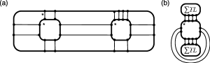
Figure 5: (a) The multiplication $\boxtimes_{k}$ (there are $k$ horizontal lines joining the input disks). (b) The trace $\tau\boxtimes_{k}\tau$ (there are $k$ loops).

Consider the associative multiplication $\boxtimes_{k}$ defined on $\oplus_{n\geq k}P_{k}$ by the tangle in Figure 5(a) and the trace $\tau\boxtimes_{k}\tau$ on $(\bigoplus_{n\geq k}P_{k},\boxtimes_{k})$ defined in Figure 5(b).

Let us call $M_{k}\boxtimes M_{k}$ the von Neumann algebra generated by this algebra in the GNS representation. These algebras are related to Popa’s symmetric enveloping algebra $M_{1}\boxtimes_{e_{0}}M_{1}^{op}$. For $k=1$ we obtain exactly the symmetric enveloping algebra, at least in the Temperley-Lieb case.

The symmetric enveloping algebra was introduced by Popa as an important analytical tool in the study of the “quantum symmetry” behind a planar algebra. For example, such analytic properties as amenability, property (T) and so on are encoded by the symmetric enveloping algebra [Pop99].

4 Random matrices and Planar algebras.

4.1 GUE and the Voiculescu trace $\tau_{TL}$

Let $M_{N\times N^{\prime}}$ denote the linear space of complex $N\times N^{\prime}$ matrices. Let $K=1,2,\dots$ be an integer, and endow $(M_{N\times N^{\prime}})^{K}$ with the Gaussian measure

$$d\mu^{(N,N^{\prime})}(A_{1},\dots,A_{K},A_{1}^{*},\dots,A_{K}^{*})\\ =\frac{1}{Z_{N}}\exp(-\frac{1}{2}NTr(\sum A_{j}^{*}A_{j}))\ dA_{1}\cdots dA_{K}dA_{1}^{*}\cdots dA_{K}^{*}.$$

Here $dA_{j}dA_{j}^{*}$ stands for Lebesgue measure on the $j$-th copy of $M_{N\times N^{\prime}}$.

A $K$-tuple of matrices $(A_{1},\dots,A_{K})$ chosen at random from $(M_{N\times N^{\prime}})^{K}$ according to this measure is called the Gaussian Unitary Ensemble (GUE).

Let $Q$ be a non-commutative polynomial in $X_{1},\dots,X_{K},X_{1}^{*},\dots,X_{K}^{*}$ which is a linear combination of monomials of the form $X_{i_{1}}X_{j_{1}}^{*}\cdots X_{i_{p}}X_{j_{p}}^{*}$ (in other words, we can think of $Q$ as an element of $(\mathcal{P},\wedge_{0})$, where $\mathcal{P}$ is the planar algebra of polynomials, see §3.6.1). For each $N,N^{\prime}$, consider the non-commutative law $\tau^{(N,N^{\prime})}$ defined by

$$\tau^{(N,N^{\prime})}(Q)\\ =\int\frac{1}{N}Tr(Q(A_{1},\dots,A_{K},A_{1}^{*},\dots,A_{K}^{*}))d\mu^{(N,N^{\prime})}(A_{1},\dots,A_{K},A_{1}^{*},\dots,A_{K}^{*}).$$

The non-commutative law $\tau^{(N,N^{\prime})}$ captures certain aspects of the random multi-matrix ensemble $(A_{1},\dots,A_{K})$. For example, the value of $\tau^{(N)}\left((A_{1}A_{1}^{*})^{p}\right)$ is the $p$-th moment of the empirical spectral measure associated to $A_{1}A_{1}^{*}$: if $\lambda_{1}<\cdots<\lambda_{N}$ are the random eigenvalues of $A_{1}A_{1}^{*}$, then

$$\tau^{(N)}\left((A_{1}A_{1}^{*})^{p}\right)=\mathbb{E}(\sum\lambda_{j}^{p}).$$

In his seminal paper [Voi91], Voiculescu showed that the laws $\tau^{(N)}$ have a limit as $N\to\infty$; rephrasing slightly he proved:

Theorem 4.2.

[Voiculescu] With the above notation, assume that $N,N^{\prime}\to\infty$ so that $N^{\prime}/N\to 1$. Then $\tau^{(N)}\to\tau_{TL}$, where $\tau_{TL}$ is the Voiculescu trace on the planar algebra of polynomials.

One can re-derive some well-known random matrix results from this theorem. For example, combining it with Lemma 3.10, one can recover convergence of singular values of block random GUE matrices to the Marcenko-Pastur law [MP67].

4.3 The case of a general planar algebra

It turns out that Theorem 4.2 also holds in the context of more general planar algebras (i.e., “in the presence of symmetry”). We now describe the appropriate random matrix ensembles.

4.3.1 Graph planar algebras

Our construction relies on the following fact [Jon01, GJS08]:

Proposition 4.4.

Every planar algebra $\mathcal{P}$ is a subalgebra (in the sense of planar algebras) of some graph planar algebra $\mathcal{P}^{\Gamma}$.

Here the graph planar algebra $\mathcal{P}^{\Gamma}$ is a planar algebra canonically associated to an arbitrary bipartite graph, taken with its Perron-Frobenius eigenvector $\mu$ (if $\mathcal{P}$ is finite depth, $\Gamma$ can be taken to be a finite graph). The spaces $\mathcal{P}_{k}^{\Gamma}$ have as linear bases the sets of closed paths of length $2k$ on $\Gamma$. The planar algebra structure is defined in a manner analogous to the case of the polynomial planar algebra, §3.6.1; see [Jon01] for details. The graph $\Gamma$ can be chosen to be finite if the planar algebra is finite depth (in particular, if $\delta<2$).

4.4.1 Random matrix ensembles on graphs

Let $\mathcal{P}$ be a planar algebra of finite depth. Thus $\mathcal{P}\subset\mathcal{P}^{\Gamma}$ for some finite bi-partite graph. Let us write $\mu(v)$ for the value of the Perron-Frobenius eigenvector at a vertex $v$ of $\Gamma$.

To an oriented edge $e$ of $\Gamma$ which starts at $v$ and ends at $w$ we associated a matrix $X_{e}$ of size $[N\mu(v)]\times[N\mu(w)]$ (here $[\cdot]$ denotes the integer part of a number). To a path $e_{1}\cdots e_{n}$ in the graph we associate the product of matrices $X_{e_{1}}\cdots X_{e_{n}}$ (here $X_{e^{o}}=X_{e}^{*}$ if $e^{o}$ is the edge $e$ but with opposite orientation).

Thus any element $W\in\bigoplus_{k}P_{k}$ is a specific expression in terms of the matrices $\{X_{e}\}_{e\in\mathcal{E}(\Gamma)}$. For example, let $\cup$ be as in Figure 3(b). Then $\cup=\sum_{e}\sqrt{\frac{\mu(v)}{\mu(w)}}X_{e}X_{e}^{*}$, the sum taken over all positively oriented edges; here $v$ and $w$ are, respectively, the start and end of $e$. Let us write $W=\sum_{v}W_{v}$, where $W_{v}$ is in the linear span of closed paths that start at $v$. Thus for example $\cup_{v}=\sum_{e}\sqrt{\frac{\mu(v)}{\mu(w)}}X_{e}X_{e}^{*}$, where the sum is taken over all edges $e$ starting at $v$.

With this notation, the expression

$$d\nu_{N}=Z_{N}^{-1}\exp(-N\sum_{v}\mu(v)Tr(\cup_{v}))\prod_{e}dX_{e}$$

makes sense and gives us a probability measure, with respect to which we can choose our random matrix ensemble $\{X_{e}\}$.

For any $Q\in P_{k}$, the expression

$$\tau_{N}(Q)=\int\sum_{v}\frac{\mu(v)}{N}Tr(P(Q_{v}(X_{e}:e\in\Gamma)))d\nu_{N}$$

gives rise to a non-commutative law on the non-commutative probability space $(\mathcal{P}^{\Gamma},\wedge_{0})$ and so in particular on $(\mathcal{P},\wedge_{0})$. We denote this restriction by $\tau^{(N)}$.

Theorem 4.5.

With the above notation, $\tau^{(N)}\to\tau_{TL}$, where $\tau_{TL}$ is the Voiculescu trace on the planar $\mathcal{P}$.

4.6 Random matrix ensembles

More generally, let us assume that we are given a non-commutative polynomial $V(t_{1},\dots,t_{K},t_{1}^{*},\dots,t_{K}^{*})$ which is a sum of monomials of the form $t_{i_{1}}t_{j_{1}}^{*}\cdots t_{i_{p}}t_{j_{p}}^{*}$. Then consider on $(M_{N\times N})^{K}$ the measure

$$d\mu_{V}^{(N)}(A_{1},\dots,A_{K},A_{1}^{*},\dots,A_{K}^{*})\\ =\frac{1}{Z_{N}}1_{\{\|A_{j}\|\leq R\}}\exp(-NTr(V(A_{1},\dots,A_{K},A_{1}^{*},\dots,A_{K}^{*})))\\ dA_{1}\cdots dA_{K}dA_{1}^{*}\cdots dA_{K}^{*},$$ (4.6.1)

where $dA_{j}$ stands for Lebesgue measure on the $j$-th copy of $M_{N\times N}$. The constant $Z_{N}$ is chosen so that $\mu_{V}^{(N)}$ is a probability measure (the cutoff $R$ insures that the support of $\mu_{V}^{(N)}$ is compact). Of course, $R=\infty$ and $V(A_{1},\dots,A_{K})=\sum A_{k}A_{k}^{*}$ corresponds to the Gaussian measure.

The measures $\mu_{V}^{(N)}$ are matrix analogs of the classical Gibbs measures $\mu_{V}=Z^{-1}\exp(-V(x))dx$.

Let us call the $K$-tuple of random matrices chosen from $(M_{N\times N}^{sa})^{K}$ at random according to this measure a random multi-matrix ensemble (see [AGZ10, Chapter 5]).

Certain properties of the random multi-matrix ensemble $A_{1},\dots,A_{K}$ is captured by the non-commutative laws $\tau_{V}^{(N)}$ defined on the algebra of non-commutative polynomials in $X_{1},\dots,X_{K},X_{1}^{*},\dots,X_{K}^{*}$ by

$$\tau_{V}^{(N)}(Q(X_{1},\dots,X_{K},X_{1}^{*},\dots,X_{K}^{*}))=\\ \int\frac{1}{N}Tr(Q(A_{1},\dots A_{K},A_{1}^{*},\dots,A_{K}^{*}))d\mu_{V}^{(N)}(A_{1},\dots,A_{K},A_{1}^{*},\dots,A_{K}^{*}).$$

4.7 Combinatorial properties of the laws $\tau_{V}^{(N)}$

Remarkably, the laws $\tau_{V}^{(N)}$ have a very nice combinatorial interpretation. Let $P$, $W_{1},\dots,W_{n}$ be a monomials, and set $V(t_{1},\dots,t_{K})=(\sum t_{j}t_{j}^{*})+\sum_{j=1}^{n}\beta_{j}W_{j}$. Define a non-commutative law $\tau_{V}$ by

$$\tau_{V}(P)=\sum_{m_{1},\dots,m_{n}\geq 0}\sum_{D}\prod_{j=1}^{n}\frac{(-\beta_{j})^{m_{j}}}{m_{j}!}$$ (4.7.1)

where the summation is taken over all planar tangles $D$ with output disk labeled by $P$ and having $m_{j}$ interior disks labeled by $W_{j}$ as in §3.6.1.

Theorem 4.8.

[Gui06, GMS06] Let $P$, $W_{1},\dots,W_{n}$ be monomials, and assume that $V(t_{1},\dots,t_{K})=(\sum t_{j}t_{j}^{*})+\sum_{j=1}^{n}\beta_{j}W_{j}$. Then for sufficiently small $\beta_{j}$,

$$\tau_{V}^{(N)}(P)=\tau_{V}(P)+O(N^{-2}).$$

The right-hand side of (4.7.1) would make sense if we were to replace $P$ and $W_{j}$ by arbitrary elements of an arbitrary planar algebra (in fact, as written, equation (4.7.1) can be taken to occur in the planar algebra of polynomials). The term $\sum t_{j}t_{j}^{*}$ correpsonds to the element $\cup$ defined in Figure 3(b). We thus make the following definition.

Definition 4.9.

Let $\mathcal{P}$ be a planar algebra, and assume that $Q\in P_{k},W_{j}\in P_{k_{j}}$, $j=1,\dots,n$ are elements of algebra $\mathcal{P}$. Let $V_{\beta}=\cup+\sum_{j}\beta_{j}W_{j}$. We define the associated free Gibbs law with symmetry $\mathcal{P}$ to be the planar algebra law

$$\tau_{V_{\beta}}(Q)=\sum_{m_{1},\dots,m_{n}\geq 0}\sum_{D}\prod_{j=1}^{n}\frac{(-\beta_{j})^{m_{j}}}{m_{j}!}Op(D)(P,\underbrace{W_{1},\dots,W_{1}}_{m_{1}},\dots,\underbrace{W_{n},\dots,W_{n}}_{m_{n}}).$$ (4.9.1)

Here the summation takes place over all planar tangles $D$ having one disk of size $k$, $m_{1}$ input disks of size $k_{1}$, $m_{2}$ disks of size $k_{2}$, etc. and no output disks.

One can check that in the case of the planar algebra of polynomials, (4.9.1) is equivalent to (4.7.1).

Theorem 4.10.

Assume that $Q\in P_{k},W_{j}\in P_{k_{j}}$, $j=1,\dots,n$ are elements of a finite-depth planar algebra $\mathcal{P}$, and let $V_{\beta}=\cup+\sum_{j}\beta_{j}W_{j}$. Then for sufficiently small $\beta$, the free Gibbs law given by (4.9.1) defines a non-negative trace on $(\oplus_{k\geq 0}P_{k},\wedge_{0})$.

We now show that the laws $\tau_{V_{\beta}}$ arise from random matrix ensembles, just as in §4.4.1 (which corresponds to $\beta=0$). Once again, we embed $\mathcal{P}$ into a graph planar algebra $\mathcal{P}^{\Gamma}$ and consider a family of random matrices $X_{e}$ of size $[N\mu(v)]\times[N\mu(w)]$ labeled by the edges $e$ of $\Gamma$ (here $[\cdot]$ denotes the integer part of a number and $\mu$ is the Perron-Frobenius eigenvector of $\Gamma$). The matrices $X_{e}$ are chosen according to the measure

$$d\nu_{N}=Z_{N}^{-1}\exp\left(-N\sum_{v}\mu(v)Tr\left((V_{\beta})_{v}\right)\right)\prod_{e}dX_{e}.$$

For any $Q\in P_{k}$, the expression

$$\tau_{N}(Q)=\int\sum_{v}\frac{\mu(v)}{N}Tr(P(Q_{v}(X_{e}:e\in\Gamma)))d\nu_{N}$$

gives rise to a non-commutative law on the non-commutative probability space $(\mathcal{P}^{\Gamma},\wedge_{0})$ and, by restriction, on $(\mathcal{P},\wedge_{0})$. We denote this restriction by $\tau_{V_{\beta}}^{(N)}$.

Theorem 4.11.

Assume that $V=\cup+\sum_{j}\beta_{j}W_{j}$ as above. Then there is a $R_{0}>0$ so that for any $R>R_{0}$, there is a $\beta_{0}>0$ so that for all $|\beta_{j}|<\beta_{0}$, $\tau_{V}^{(N)}\to\tau_{V}$ where $\tau_{V}$ is as in Theorem 4.10.

The finite-depth assumption seems to be technical in nature and is probably not necessary; it is automatically satisfied if $\delta<2$.

4.12 Example: $O(n)$ models

One application of our construction sheds some light on the construction of so-called $O(n)$ models used by in physics by Zinn-Justin and Zuber in conjunctions with questions of knot combinatorics [ZJ03, ZJZ02]. For $n$ an integer, the $O(n)$ model is the random matrix ensemble corresponding to the measure

$$Z_{N}^{-1}\exp(-NTr(V(X_{1},\dots,X_{n})))dX_{1}\cdots dX_{n}dX_{1}^{*}\cdots dX_{n}^{*}$$

where $V$ is a fourth-degree polynomial in $X_{1},\dots,X_{n},X_{1}^{*},\dots,X_{n}^{*}$ , which is invariant under the $U(n)$ action given by (3.1.1). In degree $\leq 4$, up to cyclic symmetry, the only such invariant polynomials actually lie in the copy of $TL$ contained in the algebra $\mathcal{P}^{U(n)}$ in the notation of section §3.6.1: they are linear combinations of the constant polynomial and the polynomials $\cup=\sum X_{i}X_{i}^{*}$, $\cup\cup=\sum X_{i}X_{i}^{*}X_{j}X_{j}^{*}$ and $\Cup=\sum X_{i}X_{j}^{*}X_{j}X_{i}^{*}$ (these diagrams are in $TL\subset\mathcal{P}^{U(n)}$ with parameter $\delta=n$).

Hence the $O(n)$ model is the random matrix ensemble associated to the measure

$$\mu_{(\beta,n)}^{(N)} =Z_{N}^{-1}\exp(-NTr(\sum X_{i}X_{i}^{*}+\beta_{i}\sum X_{i}X_{i}^{*}X_{j}X_{j}^{*}+\beta_{2}\sum X_{i}X_{j}^{*}X_{j}X_{i}^{*}).$$

Thus we are led to consider the laws $\tau_{\beta}$ associated to the element

$$V_{(\beta,\delta)}=\cup+\beta_{1}\cup^{2}+\beta_{2}\Cup\in TL$$

$\beta=(\beta_{1},\beta_{2})$ for each of the possible parameters $\delta\in\{2\cos\frac{\pi}{n}:n\geq 3\}\cup[2,+\infty)$. From our discussion we conclude that the limit law associated to the $O(n)$ model is exactly $\tau_{V_{(\beta,\delta=n)}}$.

But since our setting permits non-integer $\delta$, we thus gain the flexibility of considering the laws $\tau_{V(\beta,\delta)}$ for other values of $\delta$. It can be shown that the values of $\tau_{V_{(\beta,\delta=n)}}$ on a fixed element of $TL$ are analytic in $\delta$. Thus the extension we get is exactly the analytic extension from $n\in\mathbb{Z}$ to $\mathbb{C}$ considered by physicists in their analysis.

The combinatorics of the resulting law $\tau_{V}$ is governed by equation (4.9.1), which is written entirely in planar algebra terms. In particular, this shows that the $O(n)$ makes rigorous sense for any $\delta\in\{2\cos\frac{\pi}{n}:n\geq 3\}\cup[2,+\infty)$ (in the physics literature, the $O(n)$ model was used for non-integer $n$; the definition involved extending various equations analytically from $n\in\mathbb{Z}$ to $\mathbb{C}$).

It should be mentioned that $O(n)$ models were introduced in the physics literature to handle questions of knot enumerations; planar algebra interpretations of these computations are the subject of on-going research.

4.13 Properties of the limit laws $\tau_{V}$

Because of Theorem 4.11, fixing a finite-depth planar algebra $\mathcal{P}$ and a family of elements $V_{\beta}=\cup+\beta W\in\mathcal{P}$, we obtain a family laws $\tau_{\beta}=\tau_{V_{\beta}}$. These in turn give rise to a family of von Neumann algebras $W^{*}(\tau_{\beta})$ generated in the GNS representation associated to $\tau_{\beta}$. When $\beta=0$ these are free group factors (see Theorem 3.15). Voiculescu conjectured that this is also the case for $\beta\neq 0$ sufficiently small.

Using ideas from free probability theory, there has been significant progress on identifying properties of the associated Neumann algebras and $C^{*}$-algebras. The key is the following approximation result, whose proof relies on the theory of free stochastic differential equations [BS98].

Proposition 4.14.

[GS09] Assume that $\mathcal{P}$ is a the planar algebra of polynomials in $K$ variables. Let $S_{1},S_{2},\dots$ be an infinite free semicircular family generating the $C^{*}$ algebra $B$ with semicircular law $\tau$, and let $A_{\beta}=C^{*}(\tau_{\beta})$ in the GNS representation associated to $\tau_{\beta}$. Let $X_{1},\dots,X_{r}\in A_{\beta}$. Then there is a $\beta_{0}>0$ so that for all $|\beta|<\beta_{0}$ and any $\epsilon>0$ there exists an embedding $\alpha:A_{\beta}\to(A_{\beta},\tau_{\beta})*(B,\tau)$ and elements $Y_{1},\dots,Y_{r}\in B$ so that $\|\alpha(X_{j})-Y_{j}\|<\epsilon$.

Using this Proposition, many of the properties of the algebras $A_{\beta}$ can be deduced from those of the algebra $B$.

Theorem 4.15.

[GS09] Let $V=\cup+\beta W$ be an element of a finite-depth planar algebra $\mathcal{P}$. Let $\tau_{\beta}$ be the associated law on $(\mathcal{P},\wedge_{0})$. The von Neumann algebra $M=W^{*}(\tau_{\beta})$ and the $C^{*}$-algebra $A=C^{*}(\tau_{\beta})$ satisfy:

1. $M$ is a non-$\Gamma$ II₁ factor and has the Haagerup property;

2. $A$ is exact;

3. $M$ has Ozawa’s property AO and is therefore solid [Ash09].

In the case that $V$ is a polynomial potential (i.e., we are in the setting of Theorem 4.8), one can use the results of [PV82] to prove that $K_{0}(A)=0$ and that $A_{\beta}$ is projectionless. Indeed, if $p\in A$ were a non-trivial idempotent, then because of Proposition 4.14, $C^{*}(S_{1},S_{2},\dots)\subset C_{\textrm{red}}^{*}(\mathbb{F}_{2})$ would be forced to contain a non-trivial idempotent as well. This statement has random matrix consequences:

Corollary 4.16.

[GS09] Let $\mathcal{P}$ be the planar algebra of polynomials in $K$ variables, $V=V_{\beta}=\cup+\beta W\in\mathcal{P}$, and let $\tau_{\beta}=\tau_{V_{\beta}}$ be as in Theorem 4.8. Let $Q=Q^{*}\in\mathcal{P}$ be arbitrary polynomial. Let $Q^{(N)}=Q(X_{1},\dots,X_{K})$ be the random matrix obtained by evaluating $Q$ in the random matrices $(X_{1},\dots,X_{K})$ chosen according to the measure (4.6.1). Let $\mu^{(N)}$ be the expected value of the spectral measure of $Q$. Then $\mu^{(N)}\to\mu$ where $\mu$ is a measure with connected support.

Proof.

Let $Q^{(\infty)}$ denote the element of $C^{*}(\tau_{\beta})$ that corresponds to the polynomial $Q$ in the GNS construction associated to $\tau_{\beta}$. Then the law of $Q$ is exactly $\mu$. If the support of $\mu$ is not connected, the spectrum of $Q\in C^{*}(\tau_{\beta})$ is disconnected. But that means that $C^{*}(\tau_{\beta})$ contains a non-trivial projection, contradicting Theorem 4.15. ∎

It turns out that in the presence of symmetry (for non-integer $\delta$) the algebra $A_{\beta}$ may contain non-trivial projections (even at $\beta=0$). This phenomenon is not well-understood at this point, however. It would be interesting to compute the $K$-theory of the algebras $A_{\beta}$ for general planar algebras $\mathcal{P}$.

References

- [AGZ10] G. Anderson, A. Guionnet, and O. Zeitouni, An introduction to random matrices, Cambridge University Press, 2010.
- [Ash09] J. Asher, Free diffusions and property AO, Preprint, arXiv.org/0907.1314, 2009.
- [BIPZ78] E. Brézin, C. Itzykson, G. Parisi, and J. B. Zuber, Planar diagrams, Comm. Math. Phys. 59 (1978), no. 1, 35–51. MR MR0471676 (57 #11401)
- [Bis97] Dietmar Bisch, Bimodules, higher relative commutants and the fusion algebra associated to a subfactor, Operator algebras and their applications (Waterloo, ON, 1994/1995), Fields Inst. Commun., vol. 13, Amer. Math. Soc., Providence, RI, 1997, pp. 13–63. MR MR1424954 (97i:46109)
- [BS98] P. Biane and R. Speicher, Stochastic calculus with respect to free Brownian motion and analysis on Wigner space, Probab. Theory Related Fields 112 (1998), no. 3, 373–409. MR MR1660906 (99i:60108)
- [Con] A. Connes, Correspondences, unpublished notes.
- [Con94] , Noncommutative geometry, Academic Press, 1994.
- [Dyk94] K. Dykema, Interpolated free group factors, Pacific J. Math. 163 (1994), 123–135.
- [EM03] N. M. Ercolani and K. D. T.-R. McLaughlin, Asymptotics of the partition function for random matrices via Riemann-Hilbert techniques and applications to graphical enumeration, Int. Math. Res. Not. (2003), no. 14, 755–820. MR MR1953782 (2005f:82048)
- [EZJ92] B. Eynard and J. Zinn-Justin, The model on a random surface: critical points and large-order behavior, Nucl. Phys. B 386 (1992), 558–591.
- [GHJ89] F.M. Goodman, R. de la Harpe, and V.F.R. Jones, Coxeter graphs and towers of algebras, Springer-Verlag, 1989.
- [GJS08] A. Guionnet, V. Jones, and D. Shlyakhtenko, Random matrices, free probability, planar algebras and subfactors, To appear in Proceedings NCG, arXiv.org/0712.2904, 2008.
- [GJS09] , A semi-finite algebra associated to a planar algebra. Preprint arXiv.org/0911.4728, 2009.
- [GMS06] A. Guionnet and E. Maurel-Segala, Combinatorial aspects of matrix models, ALEA Lat. Am. J. Probab. Math. Stat. 1 (2006), 241–279.
- [GS09] A. Guionnet and D. Shlyakhtenko, Free diffusions and matrix models with strictly convex interaction, Geom. Funct. Anal. 18 (2009), 1875–1916.
- [Gui06] A. Guionnet, Random matrices and enumeration of maps, Proceedings Int. Cong. Math. 3 (2006), 623–636.
- [Jon83] V.F.R. Jones, Index for subfactors, Invent. Math 72 (1983), 1–25.
- [Jon99] , Planar algebras, Preprint, Berkeley, 1999.
- [Jon01] , The planar algebra of a bipartite graph, Knots in the Hellas ’98 (Delphi), World Scientific Publishing Co. Pte. Ltd., Singapore, 2001, pp. 94–117.
- [JSW08] V.F.R. Jones, D. Shlyakhtenko, and K. Walker, An orthogonal approach to the subfactor of a planar algebra, to appear in Pacific J. Math, Preprint arXiv.org/0807.4146, 2008.
- [Kos89] I. Kostov, vector model on a planar random lattice: spectrum of anomalous dimensions, Modern Phys. Lett. A 4 (1989), 217–226.
- [KS09a] V. Kodiyalam and V. S. Sunder, Guionnet-Jones-Shlyakhtenko subfactors associated to finite-dimensional Kac algebras, Preprint, arXiv.org:0901.3180, 2009.
- [KS09b] , On the Guionnet-Jones-Shlyakhtenko construction for graphs, Preprint arXiv.org:0911.2047, 2009.
- [MP67] V. A. Marčenko and L. A. Pastur, Distribution of eigenvalues in certain sets of random matrices, Mat. Sb. (N.S.) 72 (114) (1967), 507–536. MR MR0208649 (34 #8458)
- [Pop86] S. Popa, Correspondences, INCREST preprint, 1986.
- [Pop93] , Markov traces on universal Jones algebras and subfactors of finite index, Invent. Math. 111 (1993), 375–405.
- [Pop95] , An axiomatization of the lattice of higher relative commutants of a subfactor, Invent. Math. 120 (1995), no. 3, 427–445. MR 96g:46051
- [Pop99] , Some properties of the symmetric enveloping algebras with applications to amenability and property T, Documenta Mathematica 4 (1999), 665–744.
- [Pop02] , Universal construction of subfactors, J. Reine Angew. Math. 543 (2002), 39–81. MR MR1887878 (2002k:46163)
- [PS03] S. Popa and D. Shlyakhtenko, Universal properties of in subfactor theory, Acta Math. 191 (2003), no. 2, 225–257. MR MR2051399 (2005b:46140)
- [PV82] M. Pimsner and D.-V. Voiculescu, -groups of reduced crossed products by free groups, J. Operator Theory 8 (1982), 131–156.
- [Răd94] F. Rădulescu, Random matrices, amalgamated free products and subfactors of the von Neumann algebra of a free group, of noninteger index, Invent. math. 115 (1994), 347–389.
- [Spe94] R. Speicher, Multiplicative functions on the lattice of non-crossing partitions and free convolution, Math. Annalen 298 (1994), 193–206.
- [tH74] G. ’t Hooft, A planar diagram theory for strong interactions, Nuclear Phys. B 72 (1974), 461–473.
- [VDN92] D.-V. Voiculescu, K. Dykema, and A. Nica, Free random variables, CRM monograph series, vol. 1, American Mathematical Society, 1992.
- [Voi85] D.-V. Voiculescu, Symmetries of some reduced free product -algebras, Operator Algebras and Their Connections with Topology and Ergodic Theory, Lecture Notes in Mathematics, vol. 1132, Springer Verlag, 1985, pp. 556–588.
- [Voi91] , Limit laws for random matrices and free products, Invent. math 104 (1991), 201–220.
- [ZJ03] P. Zinn-Justin, The general quartic matrix model and its application to counting tangles and links, Comm. Math. Phys. 238 (2003), no. 1-2, 287–304. MR MR1990878 (2004d:57014)
- [ZJZ02] P. Zinn-Justin and J.-B. Zuber, Matrix integrals and the counting of tangles and links, Discrete Math. 246 (2002), no. 1-3, 343–360, Formal power series and algebraic combinatorics (Barcelona, 1999). MR MR1887495 (2003i:57019)