Linearly scaling direct method for accurately inverting sparse banded matrices

Abstract

In many problems in Computational Physics and Chemistry, one finds a special kind of sparse matrices, called banded matrices. These matrices, which are defined as having non-zero entries only within a given distance from the main diagonal, need often to be inverted in order to solve the associated linear system of equations. In this work, we introduce a new $\mathcal{O}(n)$ algorithm for solving such a system, with the size of the matrix being $n\times n$. We derive analytical recursive expressions that allow us to directly obtain the solution. In addition, we describe the extension to deal with matrices that are banded plus a small number of non-zero entries outside the band, and we use the same ideas to produce a method for obtaining the full inverse matrix. Finally, we show that our new algorithm is competitive, both in accuracy and in numerical efficiency, when compared with a standard method based on Gaussian elimination. We do this using sets of large random banded matrices, as well as the ones that appear in the calculation of Lagrange multipliers in proteins.

Keywords: banded matrix - sparse matrix - inversion - Gaussian elimination

1 Introduction

In this article we present the efficient formulae and subsequent algorithms to solve the system of linear equations

$$Ax=b\ ,$$ (1)

where $A$ is a $n\times n$ matrix, $x$ is the $n\times 1$ vector of unknowns, $b$ is a given $n\times 1$ vector and $A$ satisfies the equations below for known values of $m_{u},m_{l}<n$

$$A_{I,I+K} = 0\quad\forall\ K>m_{u}\ ,\quad\forall I\ ,$$ (2)

$$A_{I+L,I} = 0\quad\forall\ L>m_{l}\ ,\quad\forall I\ ,$$ (3)

i. e., $A$ is a banded matrix and (1) is a banded system. We also investigate how to solve similar systems where there are some non-zero entries not lying in the diagonal band.

Banded systems like this are abundant in computational physics and computational chemistry literature, especially because the discretization of differential equations, transforming them into finite-difference equations, often results in banded matrices [1, 2]. Many examples of this can be found in boundary value problems [3, 4, 5], in fluid mechanics [6, 7, 8], thermodynamics [9], classical wave mechanics [3], structure mechanics [10], nanoelectronics [11], circuit analysis [12], diffusion equations and Maxwell’s first-order curl equations [2]. In quantum chemistry, finite difference methods using banded matrices are used both in wavefunction formalism [13, 14, 15] and in density functional theory [16, 17]. In addition to finite-difference problems, banded systems are present in several areas, such as constrained molecular simulation [18, 19, 20], including the calculation of Lagrange multipliers in classical mechanics [21]. An important case for the calculation of Lagrange multipliers deals with molecules with angular constraints. The banded method presented here is suitable to calculate the associated Lagrange multipliers exactly and efficiently [22]. Banded matrix techniques are useful not only in linear systems, but also in linearized ones, which also appear frequently in the literature [4, 6, 7, 8, 9, 18].

The solution of a linear system with $A$ being a $n\times n$ dense matrix requires $\mathcal{O}(n^{3})$ floating point operations (a floating point operation is an arithmetic operation, like addition, subtraction, multiplication and ratio, involving real numbers which are represented in floating point notation, the customary nomenclature in computers). However, banded systems can be solved in $\mathcal{O}(nm_{u}m_{l})$ floating point operations using very simple recursive formulae, and the explicit form of $A^{-1}$ can be obtained in $\mathcal{O}(n^{2})$ floating point operations. As mentioned earlier, there exist a number of physical problems whose behaviour is described by banded systems where $m_{u},m_{l}\ll n$. This makes it possible to get large computational savings if suitable algorithms are used, what is even more important for computationally heavy problems like those in which the calculation of relevant quantities requires many iterations (Molecular Dynamics [24, 14], Monte Carlo simulations [25], quantum properties calculations via self-consistent field equations [26, 27], etc.).

In this work, we introduce a new algorithm for solving banded systems and inverting banded matrices that presents very competitive numerical properties, in many cases outperforming other commonly used techniques. Additionally, we provide the explicit recursive expressions on which the algorithm is based, thus facilitating further analytical developments. The linear ($\mathcal{O}(n)$) scaling of the presented algorithm is a remarkable feature since efficiency is commonly essential in today’s computer simulation of physical systems, specially in fields such as molecular mechanics [28, 29, 30] (using efficient force fields) and quantum ab initio methods [31, 32, 33].

The article is structured as follows: in section 2, we derive simple recursive formulae for the efficient solution of a linear banded system. These formulae enable the solution of (1) in $\mathcal{O}(nm_{u}m_{l})$ floating point operations and are suitable to be used in a serial machine. In section 3, we extend these formulae to systems where some entries outside the band are also non-zero. In section 6, we briefly discuss the differences between our new algorithm and one standard method to solve banded systems. In sec. 7 we quantitatively compare the performance of both algorithms in terms of accuracy and numerical cost. For this comparison, in sec. 7.1 we use randomly generated banded systems for inputs. In section 7.2 we apply the algorithms to the problem of calculating the Lagrange multipliers which arise when imposing holonomic constraints on proteins. Finally, in section 8, we state the most important conclusions of the work. In the Appendix we provide equations for the explicit expression of the entries of $A^{-1}$. Some remarks on the algorithmic implementation of the methods presented here, their source code and remarks on their parallelization can be found in the supplementary material.

2 Analytical solution of banded systems

One of the most common ways of solving the linear system in equation (1) is by gradually changing the different entries of the matrix $A$ to zero through the procedure of Gaussian elimination [34, 35, 36]. This procedure is based on the possibility of writing $A$ as $A=LU$, where $L$ is a lower triangular matrix and $U$ is an upper triangular matrix. This way of writing $A$, called $LU$-decomposition, is possible (i.e., $L$ and $U$ exist), if, and only if $A$ is invertible and all its leading principal minors are non-zero [37]. If one of the two matrices $L$ or $U$ is chosen to be unit triangular, i.e., with 1’s on its diagonal, the matrices not only exist but are also unique.

The analytical calculations and algorithms introduced in this work are based on a different but closely related property of $A$, namely, the possibility of finding $Q$ (a lower triangular matrix) and $P$ (an upper triangular one), so that we have

$$QAP=\mathbb{I}\quad\Rightarrow\quad A^{-1}=PQ\ ,$$ (4)

where $\mathbb{I}$ is the identity matrix.

The requirements in order for these two matrices to exist are the same as those in the $LU$-decomposition, because in fact, the two propositions are equivalent. The existence of a ‘$QP$-decomposition’ arises from the existence of the $LU$ decomposition. This trivially proved if we make $Q=L^{-1}$ and $P=U^{-1}$. The converse implication follows from the following facts. $A$ must be invertible so that equation (1) has a unique solution. The fact that its determinant ($\det A$) is different from zero and the relation $\det Q\det A\det P=\det\mathbb{I}=1$ force both $Q$ and $P$ to have non-zero determinants and therefore to be invertible. This enables one to write $A=Q^{-1}P^{-1}$, and since the inverse of a triangular matrix is a triangular matrix of the same kind, we can identify $L=Q^{-1}$ and $U=P^{-1}$ thus proving the existence of the $LU$-decomposition. This equivalence also enables one to say that, as long as one of the two matrices $Q$ and $P$ is unit triangular, the $QP$-decomposition is unique.

An important qualification of this situation is that in order to solve the system in equation (1), using $QP$ (or $LU$) decomposition is not the only option. We can also solve the system by performing a Gaussian elimination process that is based on the $QP$ (or $LU$) decomposition of a matrix $\tilde{A}$, which is obtained from $A$ by permuting its rows and/or columns. If these permutations are performed (what is called pivoting), the condition for $Q\tilde{A}P=\mathbb{I}$ (or $\tilde{A}=LU$) to hold is simply that $A$ is invertible. Typically, the algorithms obtained from the pivoting case are more stable. For the sake of simplicity, derivations of this paper deal only with the non-pivoting case (the reader should notice that pivoting can be included in the debate with minor adjustments). In the supplementary material, algorithms including and lacking pivoting can be analysed.

Let us now build the matrices $P$ and $Q$ that satisfy (4) for a given matrix $A$. When we have obtained them, they can be used to compute the inverse $A^{-1}$, and then we will be able to solve (1). However, in this section (see also ref. [38]) we will see that there is no need to explicitly build $A^{-1}$, and the information needed to calculate $P$ and $Q$ can be used in a different way to solve (1).

We begin by writing $P$ and $Q$ as follows

$$P :=P_{1}P_{2}\ldots P_{n}=\prod_{K=1}^{n}P_{K}\ ,$$ (5a)

$$Q :=Q_{n}Q_{n-1}\ldots Q_{1}=\prod_{K=n}^{1}Q_{K}\ ,$$ (5b)

being

$$P_{K}:=\left(\begin{array}[]{ccccccccc}1&&&&&&&&\\ &\ddots&&&&&&&\\ &&1&&&&&&\\ &&&\xi_{KK}&\xi_{K,K+1}&\ldots&\xi_{K,K+m_{u}}&&\\ &&&&1&&&&\\ &&&&&\ddots&&&\\ &&&&&&1&&\\ &&&&&&&\ddots&\\ &&&&&&&&1\end{array}\right)\ ,$$ (5f)

and

$$Q_{K}:=\left(\begin{array}[]{cccccccc}1&&&&&&&\\ &\ddots&&&&&&\\ &&1&&&&&\\ &&\xi_{K+1,K}&1&&&&\\ &&\vdots&&\ddots&&&\\ &&\xi_{K+m_{l},K}&&&1&&\\ &&&&&&\ddots&\\ &&&&&&&1\end{array}\right)\ ,$$ (5g)

where $K=1,\ldots,n$, and all the non-specified entries are zero. Note that $P_{K}$ equals the identity matrix except in its $K$-th row, and $Q_{K}$ equals the identity matrix except in its $K$-th column.

Now, the trick is to choose all coefficients $\xi_{IJ}$ in the preceding matrices so that we have $QAP=\mathbb{I}$ in (4) (whenever the conditions for this to be possible are satisfied; see the beginning of this section).

First we must notice that given (5f), multiplying a generic matrix $G$ (by its right) by $P_{K}$ is equivalent to adding the $K$-th column of $G$ multiplied by the corresponding $\xi$ coefficients to several columns of $G$, while at the same time multiplying the $K$-th column of the original matrix by $\xi_{KK}$:

$$(GP_{K})_{IJ} =G_{IJ}\ \qquad\textrm{for $J<K$ and $J>K+m_{u}$}\ ,$$ (5ha)

$$(GP_{K})_{IK} =G_{IK}\xi_{KK}\ ,$$ (5hb)

$$(GP_{K})_{IJ} =G_{IJ}+G_{IK}\xi_{KJ}\ \qquad\textrm{for }K<J\leq K+m_{u}\ .$$ (5hc)

If we take this into account, we can choose $\xi_{11}$ so that $(AP_{1})_{11}=1$, and $(AP_{1})_{1J}=0$ for $J=2,\ldots,n$. Given the fact that $A$ is banded (see, in particular (2, 3)), we have that

$$(AP_{1})_{11}=A_{11}\xi_{11}=1\ \Rightarrow\ \xi_{11}=1/A_{11}\ ,$$ (5hia)

$$(AP_{1})_{1J}=A_{1J}+A_{11}\xi_{1J}=0\ \Rightarrow\ \xi_{1J}=-\frac{A_{1J}}{A_{11}}\ ,\quad 1<J\leq 1+m_{u}\ .$$ (5hib)

Operating in this way, we have ‘erased’ (i.e., turned into zeros) the superdiagonal entries of $A$ that lie on its first row, and we have done this by multiplying $A$ on the right by $P_{1}$ with the appropriate $\xi_{1J}$. Then, if we multiply $(AP_{1})$ on the right by $P_{2}$ and choose the coefficients $\xi_{2J}$ in the analogous way, we can erase all the superdiagonal entries in the second row and change its diagonal entry to 1. In general, multiplying ${(AP_{1}\cdots P_{K-1})}$ by $P_{K}$ erases the superdiagonal entries of the $K$-th row of ${(AP_{1}\cdots P_{K-1})}$, and turns its diagonal $KK$ entry to 1. This procedure is called Gaussian elimination [37], and after $n$ steps, the resulting matrix is a lower unit triangular matrix $A\prod_{K=1}^{n}P_{K}=AP$.

The expression for the coefficients $\xi_{IJ}$, with $I\leq J$ and $I>1$ is more complex than (5hia) because, as a consequence of (5ha, 5hb, 5hc), whenever we multiply a matrix on the right by $P_{K}$, not only is its $K$-th row (the one we are erasing) affected, but also all the rows below are affected (the $m_{l}$ rows below in the case of a banded matrix like (4)). However, the matrix $A\prod_{L=1}^{K-1}P_{L}$ is 0 in all its superdiagonal entries belonging to the first $K-1$ rows, and multiplying it on the right by $P_{K}$ has no influence on these rows. Hence, the fact that we have chosen to erase the superdiagonal entries of $A$ from the first row to the last row allows us to express the general conditions that the $\xi$ coefficients belonging to different $P_{K}$’s must satisfy the following:

$$\left(A\prod_{K=1}^{I}P_{K}\right)_{II} =1\ ,$$ (5hija)

$$\left(A\prod_{K=1}^{I}P_{K}\right)_{IJ} =0\quad\textrm{for $I<J$}\ .$$ (5hijb)

Now, using (5hija) together with (5hb), we can derive the following expression for the coefficient $\xi_{II}$ in terms of the previous steps of the process:

$$\left(A\prod_{K=1}^{I}P_{K}\right)_{II} = \left(A\prod_{K=1}^{I-1}P_{K}P_{I}\right)_{II}=\left(A\prod_{K=1}^{I-1}P_{K}\right)_{II}\xi_{II}=1$$ (5hijk)

$$\Longrightarrow\quad\xi_{II}=\frac{1}{\left(A\prod_{K=1}^{I-1}P_{K}\right)_{II}}\ .$$

Analogously, using (5hijb) and (5hc), we can write an explicit expression for $\xi_{IJ}$ with $I<J$:

$$\left(A\prod_{K=1}^{I-1}P_{K}P_{I}\right)_{IJ} = \left(A\prod_{K=1}^{I-1}P_{K}\right)_{IJ}+\left(A\prod_{K=1}^{I-1}P_{K}\right)_{II}\xi_{IJ}=0$$

$$\Longrightarrow\quad\xi_{IJ} = -\frac{\left(A\prod_{K=1}^{I-1}P_{K}\right)_{IJ}}{\left(A\prod_{K=1}^{I-1}P_{K}\right)_{II}}=-\left(A\prod_{K=1}^{I-1}P_{K}\right)_{IJ}\xi_{II}\ .$$ (5hijl)

Also according to (5ha, 5hb, 5hc), for $I\leq J$

$$\left(A\prod_{K=1}^{L}P_{K}\right)_{IJ}=A_{IJ}+\sum_{M=J-m_{u}}^{L}\left(A\prod_{K=1}^{M-1}P_{K}\right)_{IM}\xi_{MJ}\ ,\quad I>L\ .$$ (5hijm)

Note that, in this equation we have $I>M$, which entails that $\left(A\prod_{K=1}^{M-1}P_{K}\right)_{IM}$ are subdiagonal entries. This enables one to calculate the coefficients $\xi_{IJ}$ with $I>J$, i.e., those that correspond to the matrices $Q_{K}$, once all the coefficients in the matrices $P_{K}$ have already been evaluated. We know that $AP$ is a unit lower triangular matrix. This means that its subdiagonal $I,M$ entry (with $I>M$) equals $\xi_{IJ}$, because no other changes affect this entry when multiplying $AP$ by the different $Q_{K}$’s. If $G$ is a generic matrix, then (5g) implies

$$(Q_{K}G)_{IJ} =G_{IJ}\ \qquad\textrm{for $I\leq K$ and $I>K+m_{l}$}\ ,$$ (5hijna)

$$(Q_{K}G)_{IJ} =G_{IJ}+G_{KJ}\xi_{IK}\ \qquad\textrm{for $K<I\leq K+m_{l}$, for all $J$}\ .$$ (5hijnb)

If $T$ is any unit lower triangular matrix (this is, its diagonal entries equal 1 and its superdiagonal entries are zero, $T_{II}=1$, $T_{IJ}=0$ for $I<J$), then (5g) implies

$$(Q_{K}T)_{IJ} =T_{IJ}\ \qquad\textrm{for $I\leq K$ and $I>K+m_{l}$}\ ,$$ (5hijnoa)

$$(Q_{K}T)_{IJ} =T_{IJ}+T_{KJ}\xi_{IK}\ \qquad\textrm{for $K<I\leq K+m_{l}$, $J\leq K$}\ ,$$ (5hijnob)

$$(Q_{K}T)_{IJ} =T_{IJ}\ \qquad\textrm{for $K<I\leq K+m_{l}$, $J>K$}\ .$$ (5hijnoc)

Moreover, if $S_{K-1}$ is a unit lower triangular matrix satisfying $(S_{K-1})_{IJ}=0$ for $I>J$, $J<K$, then equations (5hijnoa, 5hijnob, 5hijnoc) become

$$(Q_{K}(S_{K-1}))_{IJ}= (S_{K-1})_{IJ}\ \qquad\textrm{for $I\leq K$ and $I>K+m_{l}$}\ ,$$ (5hijnopa)

$$(Q_{K}(S_{K-1}))_{IJ}= (S_{K-1})_{IK}+(S_{K-1})_{KK}\xi_{IK}\ \ \textrm{for $K<I\leq K+m_{l}$}\ ,$$ (5hijnopb)

$$(Q_{K}(S_{K-1}))_{IJ}= (S_{K-1})_{IJ}\ \qquad\textrm{for $K<I\leq K+m_{l}$, $J>K$}\ .$$ (5hijnopc)

Multiplying $Q_{1}$ on the left by $(AP)$ erases the subdiagonal entries of the first column of $(AP)$, and multiplying $(Q_{1}AP)$ on the left by $Q_{2}$ erases the subdiagonal entries of the second column of $(Q_{1}AP)$. By repeating this procedure, multiplying $Q_{K}$ by $(Q_{K-1}\cdots Q_{1}AP)$ by the left, the subdiagonal entries of the $K$ column of $(Q_{K-1}\cdots Q_{1}AP)$ are erased. Therefore, $(Q_{K-1}\cdots Q_{1}AP)$ satisfies the conditions of $S_{K-1}$, and hence it satisfies equations (5hijnopa, 5hijnopb, 5hijnopc). The conditions for the correct erasing are:

$$(Q_{K}(Q_{K-1}\cdots Q_{1}AP))_{IK}=$$ (5hijnopq)

$$(Q_{K-1}\cdots Q_{1}AP)_{IK}+(Q_{K-1}\cdots Q_{1}AP)_{KK}\xi_{IK}=0\ \ \textrm{for $K<I\leq K+m_{l}$}\ .$$

The expressions in (5hijnopq) can be simplified. Equation (5hijnopc) implies

$$(Q_{K-1}\cdots Q_{1}AP)_{IK}=(Q_{K-1}(Q_{K-2}\cdots Q_{1}AP))_{IK}=$$

$$(Q_{K^{\prime}}(Q_{K^{\prime}-1}\cdots Q_{1}AP))_{I,K^{\prime}+1}=(Q_{K^{\prime}-1}\cdots Q_{1}AP)_{I,K^{\prime}+1}=$$

$$(Q_{K-2}\cdots Q_{1}AP)_{IK}\ ,$$ (5hijnopra)

where we have defined $K^{\prime}:=K-1$. By repeating operations like this, it is easy to obtain

$$(Q_{K-1}\cdots Q_{1}AP)_{IK}=(AP)_{IK}\ \qquad\textrm{for $K<I\leq K+m_{l}$}\ ,$$ (5hijnoprsa)

$$(Q_{K-1}\cdots Q_{1}AP)_{KK}=(AP)_{KK}=1\ .$$ (5hijnoprsb)

In addition, we must consider that (5ha, 5hb, 5hc) imply

$$\left(A\prod_{L=1}^{M-1}P_{L}\right)_{IM}=\left(A\prod_{L=1}^{n}P_{L}\right)_{IM}/\xi_{MM}=(AP)_{IM}/\xi_{MM}\qquad\textrm{for $I>M$}\ .$$ (5hijnoprst)

Using (5hijnoprsa, 5hijnoprsb, 5hijnoprst) into (5hijnopq) we obtain

$$\left(A\prod_{L=1}^{M-1}P_{L}\right)_{IM}=-\xi_{IM}/\xi_{MM}\quad\textrm{ for }I>M\ .$$ (5hiju)

If we apply this on the right hand side of (5hijm), then insert the resulting expression with $J=I$ and $L=I-1$ into (5hijk) and also insert it with $L=I-1$ into (2), we get the following recursive equations

$$\xi_{II} =\left(A_{II}-\sum_{M=I-m_{u}}^{I-1}\frac{\xi_{IM}}{\xi_{MM}}\xi_{MI}\right)^{-1}\ ,$$ (5hijva)

$$\xi_{IJ} =\xi_{II}\left(-A_{IJ}+\sum_{M=I-m_{u}}^{I-1}\frac{\xi_{IM}}{\xi_{MM}}\xi_{MJ}\right)\quad\textrm{for }I<J\ .$$ (5hijvb)

Following an analogue procedure, we obtain

$$\xi_{IJ}=\xi_{II}\left(-A_{IJ}+\sum_{M=J-m_{l}}^{J-1}\frac{\xi_{IM}}{\xi_{MM}}\xi_{MJ}\right)\quad\textrm{for }I>J\ .$$ (5hijvw)

For efficiency reasons, we prefer to define $\chi_{IJ}:=\xi_{IJ}/\xi_{II}$ for $I>J$. This makes (5hijva, 5hijvb, 5hijvw) become

$$\xi_{II} =\left(A_{II}-\sum_{M=I-m_{u}}^{I-1}\chi_{IM}\xi_{MI}\right)^{-1}\ ,$$ (5hijvxa)

$$\xi_{IJ} =\xi_{II}\left(-A_{IJ}+\sum_{M=I-m_{u}}^{I-1}\chi_{IM}\xi_{MJ}\right)\quad\textrm{for }I<J\ ,$$ (5hijvxb)

$$\chi_{IJ} =-A_{IJ}+\sum_{M=J-m_{l}}^{J-1}\chi_{IM}\xi_{MJ}\quad\textrm{for }I>J\ .$$ (5hijvxc)

The three equations above can be further modified with the aim of improving the numerical efficiency of the algorithms derived from them. The starting point for the summations in (5hijvxa) must be the value of $M$ such that both $\xi_{IM}$ and $\xi_{MJ}$ are non-zero. We must take into account that in a banded matrix the number of non zero entries above and on the left of the $I,J$ entry depends on the values of $I$, $J$:

• There are $m_{u}+(I-J)$ non-zero entries immediately above $A_{IJ}$.

• There are $m_{l}-(I-J)$ non-zero entries immediately on the left of $A_{IJ}$.

These properties are also satisfied in $A\prod_{L=1}^{K}P_{L}$ for all $K$. Therefore, if we define

$$\mu_{IJ} := \min\{m_{u}+(I-J),m_{l}-(I-J)\}\ ,$$

$$\mu^{\prime} := \min\{m_{u},m_{l}\}\ ,$$

we can re-express (5hijvxa, 5hijvxb, 5hijvxc) as

$$\xi_{II} =\left(A_{II}-\sum_{M=\max\{1,I-\mu^{\prime}\}}^{I-1}\chi_{IM}\xi_{MI}\right)^{-1}\ ,$$ (5hijvxya)

$$\xi_{IJ} =\xi_{II}\left(-A_{IJ}+\sum_{M=\max\{1,I-\mu_{IJ}\}}^{I-1}\chi_{IM}\xi_{MJ}\right) \quad\textrm{for }I<J\ ,$$ (5hijvxyb)

$$\chi_{IJ} =-A_{IJ}+\sum_{M=\max\{1,J-\mu_{IJ}\}}^{J-1}\chi_{IM}\xi_{MJ} \quad\textrm{for }I>J\ .$$ (5hijvxyc)

In the restricted but very common case in which $m_{l}=m_{u}=:m$, the previous equations become

$$\xi_{II} =\left(A_{II}-\sum_{M=max(1,I-m)}^{I-1}\chi_{IM}\xi_{MI}\right)^{-1}\ ,$$ (5hijvxyza)

$$\xi_{IJ} =\xi_{II}\left(-A_{IJ}+\sum_{M=\max\{1,J-m\}}^{I-1}\chi_{IM}\xi_{MJ}\right) \textrm{for }I<J\ ,$$ (5hijvxyzb)

$$\chi_{IJ} =-A_{IJ}+\sum_{M=\max\{1,I-m\}}^{J-1}\chi_{IM}\xi_{MJ} \textrm{for }I>J\ .$$ (5hijvxyzc)

If the matrix $A$ is symmetric ($A_{IJ}=A_{JI}$), we can avoid performing many operations simply by using

$$\chi_{IJ}=\xi_{JI}/\xi_{JJ}\ ,\qquad\textrm{for}\quad I>J\ ,$$ (5hijvxyzaa)

instead of (5hijvxyc). Equation (5hijvxyzaa) can easily be obtained from (5hijvxya) by induction.

The reader must also note that, although the coefficients $\xi_{IJ}$ have been obtained by performing the products $\prod_{K=n}^{1}Q_{K}A\prod_{L=1}^{n}P_{L}$ in a certain order, they are independent of this choice. Indeed, if we take a look to expressions (5a), (5b), (5f), and (5g), we can see that the $K$-th row (or column) is always erased before the $(K+1)$-th one. It does not matter if we apply first $Q_{K}$ or $P_{K}$ to erase the $K$ row (or column); the result of the operation will be the same. In both cases, $-G_{IK}G_{KJ}/G_{KK}$ (where $G:=\prod_{M=K-1}^{1}Q_{M}A\prod_{L=1}^{K-1}P_{L}$) is added to all the entries of $G_{IJ}$ such that $I\in\{K+1,\ldots,K+m_{l}\}$ and $J\in\{K+1,\ldots,K+m_{u}\}$. This is valid when both the $K$-th row and the $K$-th column are not erased yet. If one of them is already erased, erasing the other has no influence on $G_{IJ}$ with $I\in\{K+1,\ldots,K+m_{l}\}$ and $J\in\{K+1,\ldots,K+m_{u}\}$. In both cases $\xi_{IK}=-G_{IK}/G_{KK}$ for $I>K$, and $\xi_{KJ}=-G_{KJ}/G_{KK}$ for $J>K$. This is because all the previous rows (or columns) have been nullified before, and adding columns (or rows) has no influence on the $K$-th one.

Now, the algorithm to solve (1) can be divided into three stages (in our implementation we join together the first and second ones). Since $A^{-1}=PQ$ (4), these steps are:

1. To obtain the coefficients $\xi$.

2. To obtain the intermediate vector $c:=Qb$.

3. To obtain the final vector $x=Pc$.

Now, using the results derived above, let us calculate the expressions for the second and third steps:

Whenever we multiply a generic $n\times 1$ vector $v$ on the left by $Q_{K}$ (see (5g)), we modify its $K$-th to $(K+m_{l})$-th rows in the following way:

$$(Q_{K}v)_{I} =v_{I} \qquad\textrm{for }I\leq K,\quad I>K+m_{l}\ ,$$ (5hijvxyzaba)

$$(Q_{K}v)_{I} =v_{I}+\xi_{IK}v_{K} \qquad\textrm{for }K<I\leq K+m_{l}\ .$$ (5hijvxyzabb)

Since $Q:=Q_{n}Q_{n-1}\ldots Q_{1}$, using the expression for each of the $Q_{K}$ in (5g), and the fact that $\xi_{IJ}=0$ for $I>J+m_{l}$, we have

$$Q_{IJ} =0 \qquad\textrm{for }I<J\ ,$$ (5hijvxyzabaca)

$$Q_{II} =1\ ,$$ (5hijvxyzabacb)

$$Q_{IJ} =\sum_{M=\max\{I-m_{l},1\}}^{I-1}\xi_{IM}Q_{MJ} \qquad\textrm{for }I>J\ .$$ (5hijvxyzabacc)

where the maximum in the lower limit of the sum accounts for boundary effects and ensures that $M$ is never smaller than $1$.

From these relations between the entries of $Q$, we can get the components $c_{I}$ of the intermediate vector $c$ in the second step above:

$$c_{I} = \sum_{J=1}^{n}Q_{IJ}b_{J}=\sum_{J=1}^{I}Q_{IJ}b_{J}=b_{I}+\sum_{J=1}^{I-1}\left(\sum_{M=\max\{I-m_{l},1\}}^{I-1}\xi_{IM}Q_{MJ}\right)b_{J}$$ (5hijvxyzabacad)

$$= b_{I}+\sum_{M=\max\{I-m_{l},1\}}^{I-1}\xi_{IM}\sum_{J=1}^{I-1}Q_{MJ}b_{J}=b_{I}+\sum_{M=\max\{I-m_{l},1\}}^{I-1}\xi_{IM}c_{M}$$

$$= b_{I}+\sum_{M=\max\{I-m_{l},1\}}^{I-1}\chi_{IM}\xi_{MM}c_{M}\ .$$

In the first row of the equation above, we applied (5hijvxyzabaca), and then (5hijvxyzabacc). In the second row of the equation above, we performed a feedback in the equation.

We will now turn to the third and final step of the process, which consists of calculating the final vector $x=Pc$. Whenever we multiply a generic $n\times n$ matrix $G$ on the left by $P_{K}$ (see equation (5f)), the resulting matrix is the same as $G$ in all its rows except for the $K$-th one, which is equal to a linear combination of the first $m_{u}+1$ rows below it:

$$(P_{K}G)_{IJ} =G_{IJ} \textrm{for $I\neq K$}\ ,$$ (5hijvxyzabacaea)

$$(P_{K}G)_{KJ} =\sum_{L=K}^{\min\{K+m_{u},n\}}\xi_{KL}G_{LJ}\ ,$$ (5hijvxyzabacaeb)

where the minimum in the upper limit of the sum accounts for boundary effects and ensures that $K+L$ is never larger than $n$.

If we now use the relations above to construct $P$ as in (5a), i.e., we first take $P_{n}$ and multiply it on the left by $P_{n-1}$, then we multiply the result, $P_{n-1}P_{n}$, on the left by $P_{n-2}$, etc., we arrive to:

$$P_{II} =\xi_{II}\ ,$$ (5hijvxyzabacaeafa)

$$P_{IJ} =\sum_{K=I+1}^{\min\{I+m_{u},n\}}\xi_{IK}P_{KJ} \qquad\textrm{for }I<J\ ,$$ (5hijvxyzabacaeafb)

$$P_{IJ} =0 \qquad\textrm{for }I>J\ ,$$ (5hijvxyzabacaeafc)

meaning that every row of $P$ is a linear combination of the following rows, plus a term in the diagonal.

These expressions allow us to obtain the last equation that is needed to solve the linear system in (1):

$$x_{I} = \sum_{J=1}^{n}P_{IJ}c_{J}=\sum_{J=I}^{n}P_{IJ}c_{J}=\xi_{II}c_{I}+\sum_{J=I+1}^{n}\left(\sum_{K=I+1}^{\min\{I+m_{u},n\}}\xi_{IK}P_{KJ}\right)c_{J}$$ (5hijvxyzabacaeafag)

$$= \xi_{II}c_{I}+\sum_{K=I+1}^{\min\{I+m_{u},n\}}\xi_{IK}\sum_{J=I+1}^{n}P_{KJ}c_{J}$$

$$= \xi_{II}c_{I}+\sum_{K=I+1}^{\min\{I+m_{u},n\}}\xi_{IK}x_{K}\ .$$

Now, we can use expressions (5hijvxya), (5hijvxyb), and (5hijvxyc) in order to obtain the coefficients $\xi$, and then plug them into (5hijvxyzabacad) and (5hijvxyzabacaeafag) in order to finally solve (1).

To conclude, let us focus on the computational cost of this procedure. From (5hijvxya), (5hijvxyb), and (5hijvxyc), it follows that obtaining the coefficients $\xi$ requires $\mathcal{O}(n)$ floating point operations. Being more precise, the summations in (5hijvxya), (5hijvxyb), and (5hijvxyc), require $\mu_{IJ}$ products and $\mu_{IJ}-1$ additions ($2\mu_{IJ}-1$ floating point operations). If, without loss of generality, we consider $m_{u}\geq m_{l}$, it is easy to check that the following computational costs hold:

• Obtaining one diagonal $\xi_{II}$ takes $2\mu^{\prime}+2\simeq 2m_{u}$ floating point operations.

• Obtaining one superdiagonal coefficient $\xi_{IJ}$ (where $I<J$) takes about $2\min\{m_{l},m_{u}-(J-I)\}$ floating point operations. Hence, in order to obtain all the coefficients in a column above the diagonal, there are two sets of $\xi$’s that require a different number of operations. The lower one requires $2m_{l}$ floating point operations and the upper one requires $2(m_{u}-(J-I))$ floating point operations. All in all, obtaining $\xi_{J-I,J}$ for $I=1,\ldots,m_{u}$ takes about $m_{l}(2m_{u}-m_{l})$ floating point operations.

• In order to obtain the $\xi_{IJ}$ coefficient in a subdiagonal row ($I>J$), the number of floating point operations to be performed is $\min\{m_{u},m_{l}-(I-J)\}=m_{l}-(I-J)$; this is performed in such a way that the total number of floating point operations related to this row is approximately $m_{l}^{2}$.

Finally, obtaining all coefficients $\xi$ would require slightly less operations (due to the boundary effects) than $2nm_{u}m_{l}$ floating point operations. Once they are known (or partly known during the procedure to get them), we can obtain the solution vector $x$ using the simple recursive relationships presented in this section at a cost of $4n(m_{u}+m_{l})$ floating point operations.

3 Banded plus sparse systems

A slight modification of the calculations presented in the previous section is required to tackle systems where not all the non-zero entries are within the band. The resulting modified procedure is described in this section.

If we have

$$A^{\prime}:=A+\sum_{T=1}^{T_{max}}A^{\prime}_{R_{T}S_{T}}\Delta^{R_{T}S_{T}}\ ,$$ (5hijvxyzabacaeafah)

with $A$ banded (see eqs. (2) and (3)) and the matrix $\Delta^{R_{T}S_{T}}$ consisting of entries $(\Delta^{R_{T}S_{T}})_{IJ}=\delta_{I,R_{T}}\delta_{J,S_{T}}$, $\delta_{IJ}$ being the Kroenecker delta, we shall say that $A^{\prime}$ is a banded plus sparse matrix, and

$$A^{\prime}x=b$$ (5hijvxyzabacaeafai)

a banded plus sparse system. We call an extra-band entry any nonzero entry which does not lie in the band (this is, $A^{\prime}_{IJ}$ is an extra-band entry if it is not zero and $I<J$, $J>I+m_{u}$ or $I>J$, $J>J+m_{l}$).

In the pure banded system (section 2) only $\xi_{K,K+J}$ and $\xi_{K+I,K}$ with $K=1,\ldots,n$; $J=1,\ldots,m_{u}$; $I=1,\ldots,m_{l}$ had to be calculated. In this case, we also need to obtain

$$\xi_{IS_{T}}\quad \textrm{if $R_{T}<S_{T}$, for $I=R_{T},R_{T}+1,\ldots,S_{T}-m_{u}-1$}\ ,$$

$$\xi_{R_{T}J}\quad \textrm{if $R_{T}>S_{T}$, for $J=S_{T},S_{T}+1,\ldots,R_{T}-m_{l}-1$}\ ,$$

with $T=1,\ldots,T_{max}$.

As seen in the previous section, in order to erase (i.e., turn to 0) entry $G_{IJ}$, with $I<J$, of a generic matrix $G$, we can multiply it by a matrix $P_{I}$ (see (5f, 5ha, 5hb, 5hc)). This action adds the column $I$ (times given numbers) of matrix $G$ to other columns of $G$. This erases $G_{IJ}$, but (in general) adds nonzero numbers to the entries below it ($KJ$ entries with $K>I$). Therefore, if these entries were zero before performing the product $GP_{I}$, they will in general be nonzero after it. This implies that they will also have to be erased. Hence, erasing the extra-band entry $IJ$ of $A^{\prime}$ will not suffice; the entries $I+1,J$, $I+2,J$, $\ldots$, $J-m_{u}+1,J$ will also have to be erased. If the extra-band entry to erase $A^{\prime}_{IJ}$ is below the diagonal ($I>J$), then the $Q_{J}$ matrices (5g, 5hijna, 5hijnb) can be used to this end, since they add rows when multiplied by a generic matrix. Erasing $A^{\prime}_{IJ}$ will probably make that entries $A^{\prime}_{IK}$ with $K=J+1,\ldots,I-m_{l}-1$ become nonzero, and these entries will have to be also erased.

In order to erase the extra-band entries, the expressions presented in the previous section can be used. All extra-band entries can lie in an extended band wider than the original band. But, for the sake of efficiency, the entries in the extended band which are zero during the erasing procedure must not enter the sums for the coefficients $\xi,\chi$.

We define

$$\nu_{R_{T}I} :=\max\{R_{T},I-m_{l}\}\ ,$$ (5hijvxyzabacaeafaja)

$$\rho_{S_{T}J} :=\max\{S_{T},J+m_{u}\}\ .$$ (5hijvxyzabacaeafajb)

If $R_{T}<S_{T}$ (superdiagonal extra-band entry), in addition to coefficients appearing in (5hijvxya, 5hijvxyb, 5hijvxyc) we have to calculate

$$\xi_{R_{T}S_{T}} =-\xi_{R_{T}R_{T}}A^{\prime}_{R_{T}S_{T}}\ ,$$ (5hijvxyzabacaeafajaka)

$$\xi_{IJ} =\xi_{II}\left(\sum_{M=\nu}^{I-1}\chi_{IM}\xi_{MJ}\right) \textrm{for $R_{T}<I<S_{T}-m_{u}$}\ ;$$ (5hijvxyzabacaeafajakb)

and if $R_{T}>S_{T}$ (subdiagonal extra-band entry), in addition to coefficients appearing in (5hijvxya, 5hijvxyb, 5hijvxyc) we have to calculate

$$\xi_{R_{T}S_{T}} =-A^{\prime}_{R_{T}S_{T}}\ ,$$ (5hijvxyzabacaeafajakala)

$$\chi_{IJ} =\sum_{M=\rho}^{J-1}\xi_{IM}\chi_{MJ} \qquad\textrm{for $S_{T}<J<I-m_{l}$}\ .$$ (5hijvxyzabacaeafajakalb)

The coefficients appearing in (5hijvxyzabacaeafajaka, 5hijvxyzabacaeafajakb, 5hijvxyzabacaeafajakala, 5hijvxyzabacaeafajakalb) arise from merely applying equations (5hijvxya, 5hijvxyb, 5hijvxyc) and avoiding to include in them the coefficients $\xi$, $\chi$ which are zero due to the structure of $A^{\prime}$.

Equations (5hijvxyzabacaeafajaka, 5hijvxyzabacaeafajakb, 5hijvxyzabacaeafajakala, 5hijvxyzabacaeafajakalb) have to be modified for $I<J$ if there exist $A^{\prime}_{R_{x}S_{T}}$ with $R_{x}<R_{T}$. This is because erasing the upper non-zero entries by adding columns creates new non-zero entries below them, and the new relations must take this into account. Analogous corrections must be done for $I>J$ if there exist $A^{\prime}_{R_{T}S_{x}}$ with $S_{x}>S_{T}$. The general rule to proceed in sparse plus banded systems is to apply equations (5hijvxya, 5hijvxyb, 5hijvxyc) using the maximum $m_{u}^{\prime}$, $m_{l}^{\prime}$ so that all the nonzero entries of $A^{\prime}$ lie within the enhanched band (given by $m_{u}^{\prime}$, $m_{l}^{\prime}$), and avoid that the coefficients ($\xi$, $\chi$) which are zero take part in the sums. The coefficients $\xi_{KL}$ which are zero are those given by the following rules:

• If $K<L$, $\xi_{KL}=0$ if $A^{\prime}_{ML}=0$ for $M=1,\ldots,K$

• If $K>L$, $\xi_{KL}=0$ if $A^{\prime}_{KM}=0$ for $M=1,\ldots,L$

The computational cost of solving banded plus sparse systems scales with $n$, as long as the number of columns above the band and rows below it containing non-zero entries $A^{\prime}_{R_{T}S_{T}}$ is small ($\ll n$). The example code for an algorithm for sparse plus banded systems can be found in the supplementary material; the performance of this algorithm is presented in sec. 7.2.

4 Algorithmic implementation

Based on the expressions (5hijvxya, 5hijvxyb, 5hijvxyc, 5hijvxyzabacad, 5hijvxyzabacaeafag) derived in the paper, we have coded several different algorithms that efficiently solve the linear system in (1). The difference between the method in this paper and the most commonly used implementation of Gaussian elimination techniques, such as the ones included in LAPACK [34], Numerical Recipes in C [35], or those discussed in ref. [36] is that these methods perform an $LU$ factorization of the matrix $A$, and the coefficients $\xi$ for the Gaussian elimination are obtained in several steps, whereas the method introduced here does not perform such an $LU$ factorization, and it obtains the coefficients $\xi$ in a single step.

In order to obtain the solution of (1) we need to get the coefficients $\xi$ for Gaussian elimination as explained in section 4. That is, one diagonal coefficient for each row/column, plus $m_{u}$ coefficients in each row and $m_{l}$ coefficients in each column (except for the last ones, where less coefficients have to be calculated). More accuracy in the solution is obtained by pivoting, i.e., altering the order of the rows and columns in the process of Gaussian elimination so that the pivot (the element temporarily in the diagonal and by which we are going to divide) is never too close to zero. Double pivoting (in rows and columns) usually gives more accurate results than partial pivoting (in rows or columns). However, the former is seldom preferred for banded systems, since it requires $\mathcal{O}(n^{2})$ operations, while the latter requires only $\mathcal{O}(n)$. In the implementations described in this section, we have chosen to perform partial pivoting on rows, as in refs. [35, 34]. In the same spirit, and in order to save as much memory as possible, we store matrices by diagonals (see [35]).

We proceed as follows: For each given $I$, we obtain $\xi_{II}$ (using (5hijvxya)), and then $\xi_{JI}$ (using (5hijvxyc)) for $J=I+1,\ldots,I+m_{l}$. If $|\xi_{JI}|>|\xi_{II}|$, we exchange rows $I$ and $J$ in the matrix $A$ and in the vector $b$. This is called partial pivoting in rows, and it usually gives greater numerical stability to the solutions; in our tests of section 6 the error was lowered in two orders of magnitude by partial pivoting. Next, we calculate $\xi_{IJ}$ (using (5hijvxyb)) for $J=I+1,\ldots,I+m_{u}$. When we have calculated all the relevant coefficients $\xi$ for a given $I$, we calculate $c_{I}$ using (5hijvxyzabacad). We repeat these steps for all rows $I$, starting by $I=1$ and moving one row at a time up to $I=n$. This ordering enables us to solve the system using eqs. (5hijvxya), (5hijvxyzabacad), (5hijvxyzabacaeafag), because the superdiagonal $\xi_{IJ}$ (i.e., those with $I<J$) only require the knowledge of the coefficients with a lower row index $I$, while the subdiagonal coefficients $\xi_{IJ}$ with $I>J$ only require the knowledge of coefficients with a lower column index. We have additionally implemented a procedure to avoid performing dummy summations (i.e., those where the term to add is null), which eliminates the need for evaluating $\mu_{IJ}$ in every step. According to the pivotings performed before starting to calculate a given $\xi$, a different number of terms will appear in the summation to obtain it. This procedure uses the previous pivoting (i. e., row exchanging) information and determines how many $\xi$ coefficients have to be obtained in any row or column, and how many terms the summation to obtain them will consist of (this procedure is not indicated in the pseudo-code below for the sake of simplicity). The final step consists of obtaining $x$ from $b$ using (5hijvxyzabacaeafag).

The pseudo-code of the algorithm can be summarized as follows:

  

  // Steps 1 and 2: Calculating the coefficients $\xi$ and the vector $c$

  for ($K=1,\ K\leq n,\ K++$) do

      // Calculating the diagonal $\xi$’s:

     $\xi_{KK}=1/(A_{KK}+\sum_{M=K-\mu^{\prime}}^{K-1}\xi_{KM}\xi_{MK})$

      // Calculating the subdiagonal $\xi$’s:

     for ($I=K+1,\ I\leq I+m_{l},\ I++$) do

        $\xi_{IK}=-A_{IK}+\sum_{M=K-\mu_{IK}}^{K-1}\xi_{IM}\xi_{MK}\qquad\textrm{for }I>J$

     end for

     

     // Pivoting:

     if $\exists\ |\xi_{JI}|>|\xi_{II}|$ for $J=I+1,\ldots,I+m_{l}$ then

        for ($K=1,\ K\leq n,\ K++$) do

           $A_{IK}\leftrightarrow A_{JK}$

        end for

        $b_{I}\leftrightarrow b_{J}$

     end if

     

      // Calculating the superdiagonal $\xi$’s:

     for ($J=K+1,\ J\leq K+m_{u},\ J++$) do

        $\xi_{KJ}=-\xi_{KK}A_{KJ}+\sum_{M=K-\mu_{KJ}}^{K-1}\xi_{KM}\xi_{MJ}$

     end for

     

      // Calculating $c_{K}=(Qb)_{K}$:

     $c_{K}=b_{K}$

     for ($L=K-m_{l},\ L\leq K-1,\ L++$) do

        $c_{K}+=\xi_{K,L}c_{L}$

     end for

  end for

  

  // Step 3: Calculating $x_{K}=(Pc)_{K}=(PQb)_{K}$:

  for ($K=n,\ K\geq 1,\ K--$) do

     $x_{K}=\xi_{KK}c_{K}$

     for ($L=K+1,\ L\leq K+m_{u},\ L++$) do

        $x_{K}+=\xi_{K,L}x_{L}$

     end for

  end for

  

In the actual computer implementation we split the most external loop into three loops ($I=1,\ldots,2m$, $I=2m+1,\ldots,n-2m$, and $I=n-2m+1,\ldots,n$), because the summations to obtain the coefficients $\xi$ lack some terms in the initial and final rows. We store $A$ by diagonals in a $n\times(2m_{u}+m_{l}+1)$ matrix in order to save memory and, with the same objective, we overwrite the original entries $A_{IJ}$ with the calculated $\xi_{IJ}$ for $I\leq J$, and we store the $\xi_{IJ}$ with $I>J$ in another $n\times(2m_{l})$ matrix.

One possible modification to the algorithm presented above is to omit the pivoting. This usually leads to larger errors in the solution, but results in important computational savings. It can be used in problems where computational cost is more important than achieving a very high accuracy. In any case, one must note that the accuracy of the algorithm is typically acceptable without pivoting, so in many cases no pivoting will be necessary.

In (5hijvxyzabacaeafag) we can see that no subdiagonal coefficients ($\xi_{IJ}$ with $I>J$) are needed to obtain $x$ from $c$. In (5hijvxyzabacad), we can see that only $\xi_{IK}$ are necessary in order to obtain $c_{I}$, thus making it unnecessary to know $\xi_{LK}$ for $L<I$. Therefore, we can get rid of them once $c_{I}$ is known. Since we calculate $c_{I}$ immediately after calculating all $\xi_{IK}$, we can overwrite $\xi_{I+1,K}$ on the memory position of $\xi_{IK}$. If we do so, about one third of the memory is saved, since less coefficients must be stored, however, according to some preliminary tests, this option is also 20% slower than the simpler one in which all coefficients are stored independently.

It is also worth remarking at this point that the present state of the algorithm is not yet completely optimized at the low level and, therefore, it cannot be directly compared to the thoroughly optimized routines included in commonly used scientific libraries such as LAPACK [34]. This further optimization will be pursued in future works.

5 Parallelization

There exist many works in the literature aiming at parallelizing the calculations needed to solve a banded system [1, 10, 39, 40, 41, 42, 43, 44, 45, 46, 47, 48, 49, 50]. The decision about which one to choose, and, in particular, which one to apply to the algorithms presented in this work depends, of course, on the architecture of the machine in which the calculations are going to be performed. The choice is additionally complicated by the fact that, normally, only the number of floating point operations required by each scheme is reported in the articles. However, the number of floating point operations is known to be a poor measure of the real wall-clock performance of computer algorithms and, especially, parallel ones, for a number of reasons:

• Not all the floating point operations require the same time. For example, in currently common architectures, a quotient takes 4 times as many cycles as an addition or a product.

• A floating point operation usually requires access to several positions of memory. Each access is much slower than the floating point operation itself [51]. Moreover, the number of memory accesses does not need to be proportional to the number of floating point operations.

• Transferring information among nodes in a cluster is commonly much slower than accessing a memory position or performing a floating point operation [51].

Despite these unavoidable complexities and the fact that rigorous tests should be made in any particular architecture, two parallelizing schemes seem well suited for the method presented in this work: the one in ref. [41] for shared-memory machines and the one in ref. [10] for distributed-memory machines. The former is faster if the communication time among nodes tends to zero, whereas the latter tackles the communication time problem by significantly reducing the number of messages that need to be passed.

6 Differences with Gaussian elimination

In order to asess the performance of the method derived in the previous sections, we will present results of numerical tests of real systems. In sec. 7, we compare the absolute accuracy and numerical efficiency of our New Algorithm with those of the banded solver described in the well-known book Numerical Recipes in C [35]. However, before doing that, we can make some general remarks about the validity of the new method from the numerical point of view.

At this point, it is worth remarking that the present state of our New Algorithm for banded systems is not yet completely optimized at the low level. Therefore, it cannot be directly compared to the thoroughly optimized routines included in commonly used scientific libraries such as LAPACK [34]. This further optimization will be pursued in future works. At the current state, it is natural to compare our algorithm to an explicit, high-level, not optimized routine, such as the ones in Numerical Recipes in C [35], and the results here should be interpreted as a hint of the final performance when all levels of optimization are tackled.

Our New Algorithm (NA) is based on equations (5hijvxyza, 5hijvxyzb, 5hijvxyzc), (5hijvxyzabacad) and (5hijvxyzabacaeafag). The source code of its different versions can be found in the supplementary material. The solver of [35] (NRC) belongs to a popular family of algorithms (see, for example, [36]) which work by calculating the $\xi$ coefficients involved in the Gaussian elimination procedure in different iterations. Both for NA and for NRC, the $\xi$ coefficients required for the resolution result from the summation of several terms. For a given set of $\xi$’s, Gaussian elimination-based methods first obtain the first term of the summation of every $\xi$ then the corresponding second terms of the summations, and so on. In contrast, our method first obtains the final value of a given $\xi$ by calculating all the terms in the corresponding summation; then once a given $\xi_{IJ}$ is known, it computes $\xi_{I,J+1}$, and so on.

Both the NRC Gaussian elimination method for banded systems and our New Algorithm perform the same number of operations (i.e., the same number of additions, the same number of products, etc.). However, their efficiencies are different, as is shown in sec. 7.1. We believe this is due to the way the computers which run the algorithms access the memory positions which store the variables involved in the problem. The time that modern computers take to perform a floating point operation with two variables can be much smaller than the time required to access the memory positions of these two variables. In a modern computer, an addition or product of real numbers can take of the order of $10^{-9}$-$10^{-8}$ s. If the variables involved are stored in the cache memory, to access them can take also $10^{-9}$-$10^{-8}$ s. If they are stored in the main memory, the access can take the order of $10^{-7}$ s [52, 51]. The speed to access one position of memory is given not only by the level of memory (cache, main memory, disk, etc.) where it lies, but also by the proximity of the position of memory which was immediately read previously. Therefore, it is expected that two different algorithms will require different execution times if they access the computer memory in different ways, even if they perform the same operations with the same variables.

In the NRC Gaussian elimination procedure, a given number of floating point variables is added to each entry $A_{IJ}$. The same number of floating point variables has to be added to $A_{IJ}$ to calculate $\xi_{IJ}$ in the New Algorithm. However, the order it is done is different in both cases. In Gaussian elimination, one row of $A$ times a given number is added to another row of $A$, and this is repeated many times. For example, for erasing the subdiagonal entries of the first column of $A$, the first row (times the appropriate numbers) is added to rows 2 to $m_{l}+1$. Then, to erase the (new) second column, the (new) second row is added to rows 3 to $m_{l}+2$, and so on. Let us consider $A_{4,3}$, without a loss of generality. A given number is added to $A_{4,3}$ when the first row is added to its lower rows; after some steps, another number is added to $A_{4,3}$, when the second row is added to its lower rows. Again after some steps, another number is added to $A_{4,3}$ (when the third row is added to its lower rows). In this procedure, the memory positions that are accessed move away from the position of $A_{4,3}$, and then they come back to it, which can be suboptimal. However, in our New Algorithm, numbers are added to a memory position (say $A_{4,3}$) only once (see 5hijvxyc), making the sweeping of memory positions more efficient. Some simple tests seem to support this hypothesis. We define the following loops:

• Loop 1: (Analogous to loop of NRC-Gaussian elimination)

    for ($K=0,\ K<1000000,\ K++$) do

       for ($I=0,\ I<m_{l},\ I++$) do

          for ($J=0,\ J<m_{u}-1,\ J++$) do

              $A[m_{l}][J]+=A[I][J]$

          end for

       end for

    end for

• Loop 2: (Analogous to the loop of the New Algorithm)

    for ($K=0,\ K<1000000,\ K++$) do

       for ($I=0,\ I<m_{u}-1,\ I++$) do

           $A[m_{l}][I]+=A[0][I]+\ldots+A[m_{l}-2][I]$

       end for

    end for

The way in which Loop 1 sweeps the memory positions is analogous to that of the Gaussian elimination method (NRC), because it adds the different numbers to a given memory position ($A[m_{l}][I]$) in different iterations within the intermediate loop. The way Loop 2 sweeps the memory positions is analogous to that of the New Algorithm (NA), because it adds the different numbers to a given memory position ($A[m_{l}][I]$) just at a stretch. If we compare the times required by their executions (using $m_{u}=10$), we find the results of table 1.

Table 1: Comparison of the execution times of simple tests. The last column corresponds to data taken from sec. 7.

• $m_{l}$	$t_{\mathrm{Loop1}}$	$t_{\mathrm{Loop2}}$	$t_{\mathrm{Loop1}}/t_{\mathrm{Loop2}}$	$t_{NRC}/t_{NA}$
  3	0.379	0.169	2.243	1.145
  10	1.255	0.509	2.466	1.780
  30	3.788	1.473	2.563	2.360

This simple test gives us a clue on how the different ways to sweep memory positions can result in rather different execution times. The comparison between $t_{\mathrm{Loop1}}/t_{\mathrm{Loop2}}$ and $t_{NRC}/t_{NA}$ associated with the actual NRC and NA algorithms (without pivoting, with $N=10^{6}$ and $m_{u}=m_{l}$, see sec. 7) is merely qualitative. This is because the way the memory access takes place in Loop 1 is not exactly the same as the way the memory access takes place in NRC, nor is it the same for Loop 2 and NA (and also the $m_{u}$’s are different). The reason why the relative performance of NA vs. NRC decreases with $m$ for $m>35$ approximately can be due to the fact that in our implementation, NA uses matrices which are larger than those of NRC.

7 Numerical tests

In this section we quantitatively compare our New Algorithm with the banded solver based on Gaussian elimination of [35]. We do so by comparing the accuracy and efficiency of both algorithms for solving given systems. For the sake of generality, in the first part of this section (7.1) we use random banded systems as inputs for our tests. In the second part (7.2), we use them (plus a modified version of NA) to solve a physical problem, the calculation of the Lagrange multipliers in proteins.

7.1 Performance for generic random banded systems

In the test systems for our comparisons we imposed $m_{u}=m_{l}=m$ for the sake of simplicity. We took $n=10^{3},10^{4}$ and $10^{5}$ and $m=3,10,30,100$ and $300$ for all of them in our tests. In addition to this, we took $n=10^{6}$ with $m=3,10$ and $30$. For each given pair of values of $n$ and $m$, we generated a set of $1000$ random $n\times n$ banded matrices whose entries are null, except the diagonal ones and their first $m$ neighbours on the right and on the left. The value of these entries is a random number between $500$ and $-500$ with 6 figures. The components of the independent term (the vector $b$ in (4)) are random numbers between 0 and 1000, also with 6 figures. We tested both algorithms (from [35] and our NA) with and without pivoting. We used PowerPC 970FX 2.2 GHz machines, and no specific optimization flags were given to the compiler apart from the basic one (g++ -o solver solver.cpp). Every point in our performance plots corresponds to the mean of 1000 tests and, in each point, we used the same random system as the input for both algorithms.

We measured the efficiency of a given algorithm by using an average of its execution times for given banded systems. In the measurement of such execution times, we considered only the computation time; i.e., the measured execution times correspond only to the solution of the banded systems, and not to other parts of the code such as the generation of random matrices and vectors, the initialization of variables or the checking and the storage of the results. The measurements of the execution times start immediately after the initialization, and the clock is stopped immediately after the unknowns $x$ are calculated. The concrete information on how the measurement of times was implemented can be can be found in the source code of the programs used for our tests, which are included in the supplementary material. As is shown there, standard C libraries were used to measure the times.

The accuracy of the algorithms was determined by measuring the error of the solutions they provide ($x$). We quantified the error with the following formula, which corresponds to the normalized deviation of $Ax$ from $b$:

$$\mathrm{Error}:=\frac{\sum_{I=1}^{n}|\sum_{J=1}^{n}A_{IJ}x_{J}-b_{I}|}{\sum_{I=1}^{n}|x_{I}|}\ .$$ (5hijvxyzabacaeafajakalam)

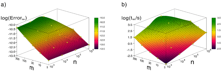
Figure 1: Properties of the New Algorithm introduced in this work, with pivoting, as a function of the size of the matrix $n$ and the width of the band $m$ in random banded test systems. a) Its accuracy, as measured by the error defined in equation (5hijvxyzabacaeafajakalam). b) Its numerical efficiency, measured by the execution time.

In the first diagrams of this section (figs. 1, 2, 3 and 4) we present the absolute and relative accuracy and efficiency of the NA and NRC algorithms for the cases with and without pivoting. In these figures, the yellow spheres represent the calculated points, which correspond to the average of 1000 tests with different input random matrices and vectors. For the sake of visual confort, interpolating surfaces have been produced with cubic splines and the $x$ and $y$ axes (labeled $n$ and $m$) are in logarithmic scale. In figures 2, 4 we compare quantities between the two algorithms; a blue plane at $z=1$ is included. Above this plane, NA is more competitive than NRC; below this plane, the converse is true.

In figure 1a, we can see that our algorithm with pivoting has very good accuracy, with the error satisfying $\mathrm{log}(\mathrm{Error})\propto\mathrm{log}(m)$. The error is proportional to a power of $m$ with a small exponent ($\simeq 1.4$). In the same figure we notice that this error is approximately independent of $n$. The execution time in the tested region (see figure 1b) is proportional to $n$ and also approximately proportional to $m^{1.7}$, not to $m^{2}$ as one would expect from the number of floating point operations ($\propto nm^{2}$). This suggests that memory access is an important time-consuming factor, in addition to floating point operations.

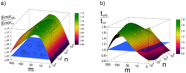
Figure 2: Comparison between the properties of the New Algorithm introduced in this work (NA) and the one in ref. [35] (NRC), both with pivoting, as a function of the size of the matrix $n$ and the width of the band $m$ in random banded test systems. a) Relative accuracy, as measured by the ratio of the errors defined in equation (5hijvxyzabacaeafajakalam). b) Relative numerical efficiency, measured by the ratio of the execution times.

In figure 2a, we can see that, if pivoting is performed, our New Algorithm is always more accurate than NRC, except for a narrow range of $m$ between 1 and 4. The typical increase in accuracy is around a 5%, reaches almost 15% for some values of $n$ and $m$. In figure 2b, we can see that, if pivoting is performed, the New Algorithm is also faster than NRC for most of the studied values of $n$ and $m$, with typical speedups of around 40% and the largest ones of almost 80%.

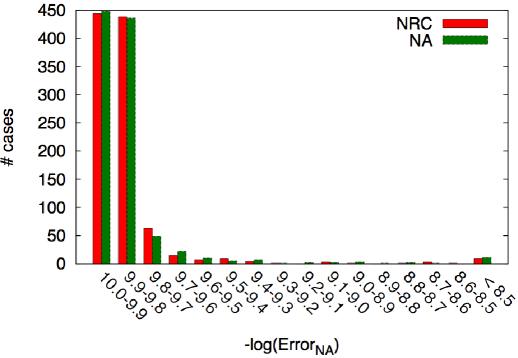
Figure 3: Histogram of the errors made by the algorithms NA and NRC for solving random banded systems without pivoting. The data corresponds to 1000 random inputs with $n=10^{5}$ and $m=10$.

If pivoting is not performed, the accuracy decreases typically by two or three orders of magnitude (but errors still remain very low, usually around $10^{-10}$).In the non-pivoting case, we also see that a few of the calculations (around 1 in 500) present errors significantly larger than the average. This probably suggests that the random procedure has produced a matrix that is close to singular with respect to the hypotheses introduced in sec. 2. In fig. 3, we show a typical example of the distribution of errors for the non-pivoting banded solvers NA and NRC in figure 3. The data corresponds to the errors of 1000 random input matrices with $n=10^{5}$ and $m=10$. In such a case, the average of the error is less representative. In this example test, the highest error in NRC is $1.57\cdot 10^{-9}$, and in NA is $2.53\cdot 10^{-9}$, although these numbers are probably anecdotal. One must also note that $99\%$ of the errors are $\mathcal{O}(10^{-10})$ or smaller. A comparison of the red and green bars in the histogram suggests that there are no big differences in the errors of both algorithms (NA and NRC) without pivoting.

Despite these problems in dealing with almost singular matrices, algorithms without pivoting have an important advantage regarding computational cost, and they can be useful for problems in which the matrices are a priori known to be well behaved. These computational savings are noticed if we compare figs. 1b, and 4a. In figure 4b, we can additionally see that the New Algorithm introduced in this work is always faster than NRC for the explored values of $n$ and $m$ if no pivoting is performed; the increase in efficiency reaching almost to a factor of 3 for some values of $n$ and $m$, and being typically around a factor of 2.

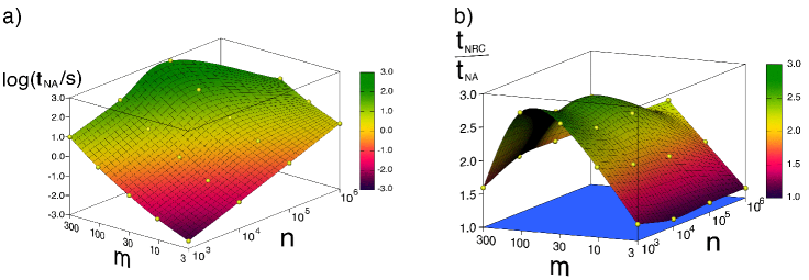
Figure 4: a) Numerical complexity of the New Algorithm introduced in this work, without pivoting, when solving random banded test systems. Execution time is shown as a function of the size of the matrix $n$ and the width of the band. b) Comparison between the numerical complexity of NA and NRC.

7.2 Analytical calculation of Lagrange multipliers in a protein

In Molecular Dynamics simulations, it is a common practice to constrain some of the internal degrees of freedom of the involved systems. This enables an increase in the simulation time step, makes the simulation more efficient, and is expected not to severely distort the value of the observable quantities calculated in the simulation [53, 54]. The bond lengths of a molecule can be constrained by including algebraic restrictions such as the following one:

$$|\vec{x}_{\alpha}-\vec{x}_{\beta}|^{2}-(a_{\alpha,\beta})^{2}=0\$$ (5hijvxyzabacaeafajakalan)

in the system of classical equations of motion of the atoms. In this expression, the positions of atoms in a molecule formed by $N_{a}$ atoms are given by $\vec{x}_{\alpha}$, $\vec{x}_{\beta}$, with $\alpha,\beta=1,\ldots,N_{a}$. The parameter $a_{\alpha,\beta}$ is the length of the bond which links atoms $\alpha$ and $\beta$.

The imposition of holonomic constraints such as (5hijvxyzabacaeafajakalan) under the assumption of the D’Alembert principle makes the so-called constraint forces appear. These forces are proportional to their associated Lagrange multipliers, which have to be calculated in order to evaluate the dynamics of the system. Proteins, nucleic acids and other biological molecules have an essentially linear topology, which makes it possible to calculate the Lagrange multipliers associated to their constrained internal degrees of freedom by solving banded systems. More explanations on how to impose constraints on molecules and on how to calculate the Lagrange multipliers in biomolecules can be found in [22].

In this section, we compare the efficiencies and accuracies of three methods to solve the banded systems associated with the calculation of Lagrange multipliers of a family of relevant biological molecules (polyalanines). The three methods we compare are:

• The Gaussian elimination algorithm for banded systems presented in [35] (NRC)

• The New Algorithm (NA) presented here, based on equations (5hijvxyza, 5hijvxyzb, 5hijvxyzc)

• A modified version of the New Algorithm presented here, which uses the methods discussed in sec. 3 and takes advantage in the symmetry of the system (i.e., it uses equation (5hijvxyzaa) instead of (5hijvxyzc))

All three methods are implemented without pivoting. The accuracies and efficiencies of the first two ones were compared in sec. 7.1 for banded matrices with random entries.

In our tests, we calculated the Lagrange multipliers of $\alpha$-helix shaped polyalanine chains (as the one displayed in fig. 5) with different numbers of residues (R). See [22] for further information on the way the systems of equations to solve were generated. In our tests, we measured the error as calculated with (5hijvxyzabacaeafajakalam), as well as the execution time of the algorithms. We ran them in a MacBook6,1 with a 2.26 GHz Intel Core 2 Duo processor.

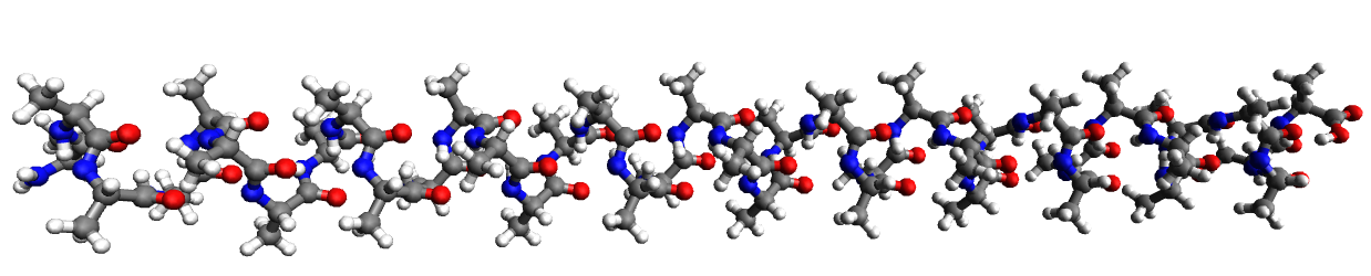
Figure 5: Polyalanine chain of 40 residues in a $\alpha$-helix shape. White spheres indicate H atoms, dark spheres indicate C atoms, blue spheres indicate N atoms and red spheres indicate O atoms. The covalent bonds appear as rods connecting them. Diagram made with Avogadro [55].

The results are displayed in figures 6 and 7.

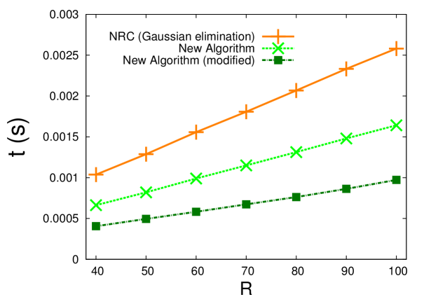
Figure 6: Comparison of the execution times (t) of different algorithms to solve banded systems in the calculation of the Lagrange multipliers in a polyalanine chain of R residues. Vertical crosses: NRC (Gaussian elimination); Diagonal crosses: NA; Squares: modified New Algorithm.

For all the polypeptide lengths represented in fig. 6, the execution time of the Gaussian elimination algorithm (NRC) is about 1.57 times the execution time of the New Algorithm ($1.57\pm 0.01$). The modified New Algorithm (squares in figures 6 and 7) is about 2.70 times faster than the NRC algorithm. These results were the expected results for the used values of $n$, $m_{u}$ and $m_{l}$ ($m_{u}=m_{l}=m=6$, $n=10\mathrm{R}+2$), according to the tendencies observed in the previous section. Higher values of $m$ are expected to result in better relative efficiency of the New Algorithm (see sec. 7.1). A situation that we can meet, for example, if not only bond lengths, but also bond angles, are constrained, and if the branches of the molecule are longer (for example, the side chains of the arginine residue are longer than the side chains of the alanine residue).

The errors made by the three tested algorithms are displayed in fig. 7.

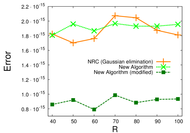
Figure 7: Comparison of the errors made by different algorithms in the solution of banded systems for the calculation of the Lagrange multipliers in a polyalanine chain of R residues. Vertical crosses: NRC (Gaussian elimination); diagonal crosses: NA; squares: modified New Algorithm.

As expected for the case without pivoting (see sec. 7.1), the errors of the NRC and NA algorithms are similar, and both are very small (similar to the errors arisen from the finite machine precision). The error of the modified version of the New Algorithm is typically less that half of the error of the other two methods. This can be due to the fact that the modified version uses equation (5hijvxyzaa) instead of (5hijvxyzc). Therefore, fewer numbers (about half of them) are present in the calculation, and hence fewer potential sources of error are present.

We conclude that, for the systems tested in this section, the new algorithm introduced in this work is competitive both in accuracy and in computational efficiency when compared with a standard method for inverting banded matrices. This holds true both with and without pivoting. We stress we are comparing two algorithms which are not yet thoroughly optimized (as LAPACK is).

8 Concluding remarks

In this paper, we have introduced a new linearly scaling method to invert the banded matrices that so often appear in problems of Computational Physics, Chemistry and other disciplines. We have proven that this new algorithm is capable of being more accurate than standard methods based on Gaussian elimination at a lower computational cost, which opens the door to its use in many practical problems, such as the ones described in the introduction.

Moreover, we have produced the analytical expressions that allow us to directly obtain, in a recursive manner, the solution to the associated linear system in terms of the entries of the original matrix. To have these explicit formulae (which have also been presented for the calculation of the full inverse matrix in the Appendix) at our disposal not only simplifies the task of coding the needed computer algorithms, but it may also be useful to facilitate analytical developments in the problems in which banded matrices appear.

In addition, we have checked its performance for general trial systems, and proven its usefulness for real physical problems (calculations on dynamics of proteins).

Aknowledgments

The authors would like to thank J. L. Alonso, G. Ciccotti, J. M. Peña, S.R. Christensen and Á. Rubio for illuminating discussions and useful advice, and M. García-Risueño for helping with the plots, as well as the staff of Caesaraugusta supercomputing facility (RES), where the test calculations of this paper were run. This work has been supported by the research projects E24/3 (DGA, Spain), FIS2009-13364-C02-01 (MICINN, Spain) 200980I064 (CSIC, Spain) and ARAID and Ibercaja grant for young researchers (Spain). P. G.-R. is supported by a JAE PREDOC grant (CSIC, Spain).

Appendix A Inverse of a banded matrix

In the previous sections, we proved that the banded linear system of $n$ equations with $n$ unknowns in (1) can be solved in order $n$ operations. Sometimes, we are interested in obtaining the inverse matrix $A^{-1}$ itself. We can do this in order $n^{2}$ operations using the same kind of ideas discussed in the main body of the article. It should be stressed that the explicit inverse of an arbitrary banded matrix usually cannot be obtained in $\mathcal{O}(n)$ floating point operations, since the inverse of a banded matrix has $n^{2}$ entries and it is not, in general, a banded matrix itself (an exception to this is a block diagonal matrix). In order to obtain an efficient way to invert $A$, we will derive some recursive relations between the rows of $P$ (and $Q$). To this end, we will first calculate the explicit expression of the entries of these matrices.

Using eqs. (5a), (5f), and (5g), from which (5ha, 5hb, 5hc) and (5hijvxyzaba) follow, and after some straightforward but long calculations, one can show that the aforementioned entries satisfy

$$P_{IJ} =\xi_{JJ}\sum_{c\in C_{I,J,m_{u}}^{\uparrow}}\prod_{(K,L)\in c}\xi_{KL} \textrm{for $I<J$}\ ,$$ (5hijvxyzabacaeafajakalaoa)

$$P_{II} =\xi_{II}\ ,$$ (5hijvxyzabacaeafajakalaob)

$$P_{IJ} =0 \textrm{for $I>J$}\ ,$$ (5hijvxyzabacaeafajakalaoc)

and

$$Q_{IJ} =\sum_{c\in C_{I,J,m_{l}}^{\downarrow}}\prod_{(K,L)\in c}\xi_{KL} \textrm{for $I>J$}\ ,$$ (5hijvxyzabacaeafajakalaoapa)

$$Q_{II} =1\ ,$$ (5hijvxyzabacaeafajakalaoapb)

$$Q_{IJ} =0 \textrm{for $I<J$}\ .$$ (5hijvxyzabacaeafajakalaoapc)

We call the summations appearing in the first line of each of these groups of expressions jump summations. There are two jump summations here, one from $I$ to $J$ with increasing indices ($\uparrow$) and $m_{u}$ neighbours, and a jump summation from $I$ to $J$ with decreasing indices ($\downarrow$) and $m_{l}$ neighbours, respectively. The jump summation provides us with an explicit expression for all entries in $A^{-1}$, without the need to recursively refer to other entries. This can be useful in order to parallelize its calculation.

As it can be seen in the expressions, that each product in the sums contains a number of coefficients $\xi_{KL}$. The pairs of indices $(K,L)$ which are included in a given product are taken from a set $c$. In turn, each term of the sum corresponds to a different set of pairs of indices $c$ drawn from a set of sets of pairs of indices $C_{I,J,m_{u}}^{\uparrow}$ (in the case of $P_{IJ}$) or $C_{I,J,m_{l}}^{\downarrow}$ (in the case of $Q_{IJ}$). Therefore, the only detail that remains to understand these ‘jump summations’ is to specify which are the elements of these latter sets.

A given element $c$ of either $C_{I,J,m_{u}}^{\uparrow}$ or $C_{I,J,m_{l}}^{\downarrow}$ can be expressed as

$$c=\{(K_{1},L_{1}),(K_{2},L_{2}),\ldots,(K_{S},L_{S})\}\ ,$$ (5hijvxyzabacaeafajakalaoapaq)

in such a way that $C_{I,J,m_{u}}^{\uparrow}$ comprises all possible $c$’s that comply with a number of rules:

• $K_{1}=I$, and $L_{S}=J$.

• $K_{r}<L_{r}$, for $r=1,\ldots,S$.

• $K_{r+1}=L_{r}$, for $r=1,\ldots,S$.

• $L_{r}-K_{r}\leq m_{u}$, for $r=1,\ldots,S$.

Let us see an example:

$$\sum_{c\in C_{3,6,2}^{\uparrow}}\prod_{(K,L)\in c}\xi_{KL} = \xi_{3,4}\xi_{4,5}\xi_{5,6}+\xi_{3,4}\xi_{4,6}+\xi_{3,5}\xi_{5,6}\ .$$ (5hijvxyzabacaeafajakalaoapar)

The rules to determine the elements of $C_{I,J,m_{l}}^{\downarrow}$ are analogous to the ones above but they take into account that the indices decrease:

• $K_{1}=I$, and $L_{S}=J$.

• $K_{r}>L_{r}$, for $r=1,\ldots,S$.

• $K_{r+1}=L_{r}$, for $r=1,\ldots,S$.

• $K_{r}-L_{r}\leq m_{l}$, for $r=1,\ldots,S$.

An example would be:

$$\sum_{c\in C_{5,1,3}^{\downarrow}}\prod_{(K,L)\in c}\xi_{KL} = \xi_{5,4}\xi_{4,3}\xi_{3,2}\xi_{2,1}+\xi_{5,3}\xi_{3,2}\xi_{2,1}+\xi_{5,4}\xi_{4,2}\xi_{2,1}$$ (5hijvxyzabacaeafajakalaoapas)

$$\mbox{}+\xi_{5,4}\xi_{4,3}\xi_{3,1}+\xi_{5,3}\xi_{3,1}+\xi_{5,2}\xi_{2,1}+\xi_{5,4}\xi_{4,1}\ .$$

If we first focus on $P$, it is easy to see that, according to the properties of the jump summation, we have

$$\sum_{c\in C_{I,J,m_{u}}^{\uparrow}}\prod_{(K,L)\in c}\xi_{KL} = \xi_{I,I+1}\sum_{c\in C_{I+1,J,m_{u}}^{\uparrow}}\prod_{(K,L)\in c}\xi_{KL}$$ (5hijvxyzabacaeafajakalaoapat)

$$\mbox{}+\xi_{I,I+2}\sum_{c\in C_{I+2,J,m_{u}}^{\uparrow}}\prod_{(K,L)\in c}\xi_{KL}$$

$$\mbox{}+\ldots+\xi_{I,I+m_{u}}\sum_{c\in C_{I+m_{u},J,m_{u}}^{\uparrow}}\prod_{(K,L)\in c}\xi_{KL}\ .$$

If we insert a multiplicative factor $\xi_{JJ}$ at both sides and use (5hijvxyzabacaeafajakalaoa), this equation becomes equation (5hijvxyzabacaeafa) obtained in sec. 2:

$$P_{IJ}=\sum_{K=I+1}^{\min\{I+m_{u},n\}}\xi_{IK}P_{KJ}\qquad\textrm{for }I<J\ .$$

An analogous expression for $Q$ can be obtained in a similar way:

$$Q_{IJ}=\sum_{L=J+1}^{\min\{J+m_{l},n\}}Q_{IL}\xi_{LJ}\qquad\textrm{for }I>J\ .$$

Now, if we define $\mu_{1}:=\min\{m_{u},J-I\}$, and $\mu_{2}:=\min\{m_{l},I-J\}$, since $A^{-1}=PQ$ (see (4)), we have that

$$(A^{-1})_{IJ} = (PQ)_{IJ}=\sum_{K=1}^{n}P_{IK}Q_{KJ}=\sum_{K=J}^{n}P_{IK}Q_{KJ}=$$ (5hijvxyzabacaeafajakalaoapau)

$$= \sum_{K=J}^{n}\left(\sum_{L=I+1}^{I+\mu_{1}}P_{LK}\xi_{IL}\right)Q_{KJ}=\sum_{L=I+1}^{I+\mu_{1}}\xi_{IL}\left(\sum_{K=J}^{n}P_{LK}Q_{KJ}\right)$$

$$= \sum_{L=I+1}^{I+\mu_{1}}\xi_{IL}(A^{-1})_{LJ}\qquad\textrm{for $I<J$}\ ,$$

which is a recursive relationship for the superdiagonal entries of $A^{-1}$.

Performing similar computations, we have

$$(A^{-1})_{II} = \xi_{II}+\sum_{L=I+1}^{I+\mu_{1}}\xi_{IL}(A^{-1})_{LJ}=\xi_{II}+\sum_{L=J+1}^{J+\mu_{2}}\xi_{LJ}(A^{-1})_{IL}\ ,$$ (5hijvxyzabacaeafajakalaoapav)

$$(A^{-1})_{IJ} = \sum_{L=J+1}^{J+\mu_{2}}\xi_{LJ}(A^{-1})_{IL}\qquad\textrm{for $I>J$}\ .$$ (5hijvxyzabacaeafajakalaoapaw)

Using the last three equations, we can easily construct an algorithm to compute $A^{-1}$ in $\mathcal{O}(n^{2})$ floating point operations. This algorithm would first calculate $(A^{-1})_{nn}=\xi_{nn}$. Then it would use (5hijvxyzabacaeafajakalaoapau) to obtain, in this order, $(A^{-1})_{n-1,n}$, $(A^{-1})_{n-2,n}$, $\ldots$, $(A^{-1})_{1n}$. These are the superdiagonal ($I<J$) entries of the $n$-th column. Then, it would use (5hijvxyzabacaeafajakalaoapaw) to obtain, in this order, $(A^{-1})_{n,n-1}$, $(A^{-1})_{n,n-2}$, $\ldots$, $(A^{-1})_{n1}$, i.e., the subdiagonal ($I>J$) entries of the $n$-th row. Once the $n$ row and column of $A^{-1}$ are known, $(A^{-1})_{n-1,n-1}$ can be obtained with (5hijvxyzabacaeafajakalaoapav). Then (5hijvxyzabacaeafajakalaoapau) and (5hijvxyzabacaeafajakalaoapaw) can be used to obtain the entries of this ($n-1$) column and row, respectively. When calculating the entries of a column $J$, i.e., $\xi_{KJ}$ with $K<J$, $\xi_{LJ}$ is always obtained before $\xi_{L-1,J}$. When calculating the entries of a row $I$, i.e., $\xi_{IK}$ with $I>K$, $\xi_{IK}$ is always obtained before $\xi_{I,K-1}$. This procedure can be repeated for all rows and columns of $A^{-1}$, and the calculation of the $K$-th row and column can be performed in parallel.

References

References

- [1] Dongarra J and Johnson S L 1987 Parallel Computing 5 219–246
- [2] Hyman J, Morel J, Shashkov M and Steinberg S 2002 Computational Geosciences 6 333–352
- [3] Shaw R E and Garey L E 1997 International Journal of Computer Mathematics 65, 1-2 121–129
- [4] Paprzycki M and Gladwell I 1991 Parallel Computing 17 133–153
- [5] Wright S J 1992 SIAM J. Sci. Stat. Comput. 13 742–764
- [6] Briley W R and McDonald H 1977 JCOP 24, 4 372–397
- [7] Ariel P D 1992 Acta Mechanica 103 31–43
- [8] Haddad O M, Al-Nimr M A and Shatnawi G H 2008 Selected Papers from the WSEAS Conferences in Spain, September 2008 Santander, Cantabria, Spain
- [9] Haddad O, Abuzaid M and Al-Nimr M 2004 Entropy 6, (5) 413–416
- [10] Polizzi E and Shameh A H 2006 Parallel Computing 32 177–194
- [11] Polizzi E and Ben Abdallah N 2004 Journal of Computational Physics 202, 1 150–180
- [12] Lumsdaine A, White J, Webber D and Sangiovanni-Vincentelli A 1988 Research Laboratory of Electronics Dept. of Electrical Engineering and Computer Science Massachusetts Institute of Technology Cambridge, MA 02139, CH2657-5/88/0000/0308 01.000 1988IEEE
- [13] Sanz-Serna J M and Christie I 1986 Journal of Computational Physics 67, 2 348–360
- [14] Guantes R and Farantos S C 1999 Journal of Chemical Physics 111, 24 10827–10835
- [15] Guardiola R and Ros J 1999 Journal of Computational Physics 111, 24 374–389
- [16] Castro A, Appel H, Oliveira M, Rozzi C A, Andrade X, Lorenzen F, Marques M A L, Gross E K U and Rubio A 2006 Phys. Stat. Sol 243 2465
- [17] Marques M A L, Castro A, Bertsch G F and Rubio A 2003 Comp. Phys. Comm. 151 60
- [18] Ryckaert J P, Ciccotti G and Berendsen H J C 1977 J. Comput. Phys. 23 327–341
- [19] Alvarez-Estrada R F and Calvo G F 2004 Journal of Physics: Condensed Matter 16 S2037
- [20] Calvo G F and Alvarez-Estrada R F 2005 Journal of Physics: Condensed Matter 17 7755
- [21] Mazars M 2007 J. Phys. A: Math. Theor. 40, 8 1747–1755
- [22] García-Risueño P, Echenique P and Alonso J L 2011 J. Comput. Chem. 32 3039–3046
- [23] Strassen V 1969 Numerische Mathematik 13 354––356
- [24] Alonso J L, Andrade X, Echenique P, Falceto F, Prada-Gracia D and Rubio A 2008 Phys. Rev. Lett. 101 096403
- [25] Hastings W K 1970 Biometrika 57, 1 97–109
- [26] Echenique P and Alonso J L 2007 Mol. Phys. 105 3057–3098
- [27] Gritsenko O V, Rubio A, Balbás L C and Alonso J A 1993 Phys. Rev. A 47 1811–1816
- [28] Pearlman D A, Case D A, Caldwell J W, Ross W R, Cheatham III T E, DeBolt S, Ferguson D, Seibel G and Kollman P 1995 Comp. Phys. Commun. 91 1–41
- [29] Cavasotto C N and W Orry A J May Current Topics in Medicinal Chemistry 7 1006–1014
- [30] Anisimov V M and Cavasotto C N 2011 Journal of Computational Chemistry 32 2254–2263
- [31] Hine N, Haynes P, Mostofi A, Skylaris C K and Payne M 2009 Computer Physics Communications 180 1041 – 1053
- [32] Soler J M, Artacho E, Gale J D, García A, Junquera J, Ordejón P and Sánchez-Portal D 2002 Journal of Physics: Condensed Matter 14 2745
- [33] Gillan M, Bowler D, Torralba A and Miyazaki T 2007 Computer Physics Communications 177 14 – 18 proceedings of the Conference on Computational Physics 2006 - CCP 2006, Conference on Computational Physics 2006
- [34] Anderson E, Bai Z and Bischof C e a (1999) LAPACK User’s Guide release 3.0 ed (Philadelphia: SIAM)
- [35] Press W H, Teukolsky S A, Vetterling W T and Flannery B P (2007) Numerical recipes. The art of scientific computing 3rd ed (New York: Cambridge University Press)
- [36] Wakins D S 1991 Fundamentals of Matrix Computations 2nd ed (New York: Wiley Inter-Science)
- [37] Golub G H and Van Loan C F (eds) 1993 Matrix Computations 2nd ed (Baltimore and London: The Johns Hopkins University Press)
- [38] Castro A, Marques M A L and Rubio A 2004 J. Chem. Phys. 121 3425–3433
- [39] Chandrasekaran S and Gu M 2003 SIAM Journal on Matrix Analysis and its Applications 25(2) 373–384
- [40] Bini D A and Meini B 1999 SIAM J. Matrix Anal. Appl. 20 700––719
- [41] Meier U 1985 Parallel Computing 2 33–23
- [42] Zhang H and Moss W F 1994 Parallel Computing 20, 8 1089–1105
- [43] Lawrie D H and Sameh A H 1984 ACM Transactions on Mathematical Software 10, 2 185–195
- [44] Johnson S L 1985 ACM Transactions on Mathematical Software 11 271–288
- [45] Chen S C, Kuck D J and Sameh A H 1978 ACM Transactions on Mathematical Software 4 270–277
- [46] Evans D J and Hatzopoulos M 1976 The Computer Journal 19, 2 184–187
- [47] Garey L E and Shaw R E 2000 Applied Mathematics and Computation 5, 311 133–143
- [48] Arbenz P and Gander W 1994 Technical Report TR 221, Inst. for Scientific Comp., ETH, Zürich
- [49] Golub G H, Sameh A H and Sarin V 2001 Numerical linear algebra with applications 8 297–316
- [50] Dongarra J and Sameh A H 1984 Parallel Computing 1 223–235
- [51] Hennessy J L and Patterson D A 2003 Computer Architecture, A Quantitative Approach 3rd ed (San Mateo, CA: Morgan Kaufmann - Elsevier)
- [52] Hager G and Wellein G 2011 Introduction to High Performance Computing for Scientists and Engineers 1st ed (CRC Press - Taylor & Francis Group)
- [53] Leimkuhler B and Reich S 2004 Simulating Hamiltonian dynamics 1st ed (Cambridge University Press - Cambridge monographs on applied and computational Mathematics)
- [54] Hess B, Bekker H, Berendsen H J C and Fraaije J G E M 1997 J. Comput. Chem. 18 1463–1472
- [55] 2010 Avogadro: an open-source molecular builder and visualization tool. version 1.0.1 http://avogadro.openmolecules.net/