Slow quench dynamics of the Kitaev model: anisotropic critical point and effect of disorder

Abstract

We study the non-equilibrium slow dynamics for the Kitaev model both in the presence and the absence of disorder. For the case without disorder, we demonstrate, via an exact solution, that the model provides an example of a system with an anisotropic critical point and exhibits unusual scaling of defect density $n$ and residual energy $Q$ for a slow linear quench. We provide a general expression for the scaling of $n$ ($Q$) generated during a slow power-law dynamics, characterized by a rate $\tau^{-1}$ and exponent $\alpha$, from a gapped phase to an anisotropic quantum critical point in $d$ dimensions, for which the energy gap $\Delta_{\vec{k}}\sim k_{i}^{z}$ for $m$ momentum components ($i=1..m$) and $\sim k_{i}^{z^{\prime}}$ for the rest $d-m$ components ($i=m+1..d$) with $z\leq z^{\prime}$: $n\sim\tau^{-[m+(d-m)z/z^{\prime}]\nu\alpha/(z\nu\alpha+1)}$ ($Q\sim\tau^{-[(m+z)+(d-m)z/z^{\prime}]\nu\alpha/(z\nu\alpha+1)}$). These general expressions reproduce both the corresponding results for the Kitaev model as a special case for $d=z^{\prime}=2$ and $m=z=\nu=1$ and the well-known scaling laws of $n$ and $Q$ for isotropic critical points for $z=z^{\prime}$. We also present an exact computation of all non-zero, independent, multispin correlation functions of the Kitaev model for such a quench and discuss their spatial dependence. For the disordered Kitaev model, where the disorder is introduced via random choice of the link variables $D_{n}$ in the model’s Fermionic representation, we find that $n\sim\tau^{-1/2}$ and $Q\sim\tau^{-1}$ ($Q\sim\tau^{-1/2}$) for a slow linear quench ending in the gapless (gapped) phase. We provide a qualitative explanation of such scaling.

I Introduction

Non-equilibrium dynamics of quantum systems near quantum critical points has been a subject of intense study in recent years pol1 ; dziar1 . During such dynamics, a quantum system passes from one gapped phase to another via time evolution of a Hamiltonian parameter $\lambda$ with a rate $\tau^{-1}$ and an exponent $\alpha$ ($\lambda(t)=\lambda_{0}|t/\tau|^{\alpha}{\rm Sgn}(t)$, where ${\rm Sgn}(x)=1(-1)$ for $x>(<)\,0$) through an intermediate quantum critical point at $\lambda=0$. At the critical point, the energy gap vanishes as $\Delta(\vec{k})\sim|\vec{k}|^{z}$ where $z$ is the dynamical critical exponent. Thus the dynamics becomes non-adiabatic around a region near this point and the system fails to remain at the instantaneous ground state leading to formation of defects kibble1 ; zurek1 ; pol2 ; others1 ; sen1 ; pol3 ; sendutta . The density of these defects ($n$) and the residual energy produced in the process ($Q$) scale with universal exponents: $n\sim\tau^{-\nu d\alpha/(z\nu\alpha+1)}$ and $Q\sim\tau^{-(d+z)\nu\alpha/(z\nu\alpha+1)}$, where $\nu$ is the correlation length exponent and $d$ is the system dimension pol2 ; sen1 . It is well-known that scaling laws do not change if the dynamics terminate at the critical point pol3 . All of the above-mentioned studies apply to isotropic critical points where the scaling of the energy gap with the momentum is described by a single exponent $z$. Recently, the anisotropic Dirac model with an anisotropic critical point is studied and it was shown that one needs multiple exponents to describe the scaling of the energy gap dutta1 . However such studies have not been carried out in the context of the Kitaev model and generic expressions for the scaling laws for $n$ and $Q$ for such critical points in arbitrary dimensions have not been provided. Also, the effect of disorder on defect production in models, where the Harris criterion allows for the existence of a sharp quantum phase transition, has not been studied so farsachdev1 .

In this work, we study several aspects of non-equilibrium slow dynamics in the vicinity of both anisotropic critical points and critical points in the presence of disorder with specific focus on the 2D Kitaev model which provides an explicit realization of both the cases. First, we derive a generic model-independent expression for the scaling of $n$ and $Q$ for such dynamics which takes a $d$-dimensional system from a gapped phase to the vicinity of an anisotropic critical point. We consider a scenario where the energy gap $\Delta_{\vec{k}}$ vanishes as $k_{i}^{z}$ for $m$ momentum components ($i=1..m$) and as $k_{i}^{z^{\prime}}$ for the rest $d-m$ components ($i=m+1..d$) with $z^{\prime}\geq z$ at the critical point and show that the time-evolution of the Hamiltonian parameter $\lambda(t)$, which brings the system at the critical point at $t=0$, leads to novel scaling laws for $n$ and $Q$:

$$n\sim\tau^{-[m+(d-m)z/z^{\prime}]\nu\alpha/(z\nu\alpha+1)},$$

$$Q\sim\tau^{-[(m+z)+(d-m)z/z^{\prime}]\nu\alpha/(z\nu\alpha+1)}.$$ (1)

Our results reproduce their well-known counterparts for the isotropic case ($z=z^{\prime}$) as special cases. We also show, by exact analytical solution for linear time evolution ($\alpha=1$), that the two-dimensional (2D) Kitaev model, in the absence of disorder, provides an explicit realization of the scaling laws mentioned above with $d=z^{\prime}=2$ and $m=\nu=z=1$ leading to $n\sim\tau^{-3/4}$ and $Q\sim\tau^{-5/4}$. We also corroborate the scaling laws mentioned above by numerical studies of the Kitaev model for arbitrary power-law time evolution. Second, we compute all independent multispin correlation function of the Kitaev model subsequent to a slow linear ramp which takes the system from a gapped phase to the vicinity of the anisotropic critical point, demonstrate their anisotropic nature, and discuss their spatial dependence. Third, we study non-equilibrium slow linear dynamics of the disordered Kitaev model where disorder is introduced via random choice of the fields $D_{\vec{n}}$ in the Fermionic representation of the model, and show, by explicit numerical calculation, that the defect production for such a dynamics obeys a different scaling law compared to its disorder free counterpart: $n\sim\tau^{-1/2}$ and $Q\sim\tau^{-1}$ ($Q\sim\tau^{-1/2}$) for a quench ending in the gapless (gapped) phase. We provide a qualitative explanation for such defect production.

The organization of the rest of the work is as follows. In Sec. II, we discuss scaling laws for defect density and residual energy for dynamics near an anisotropic critical point in the absence of disorder and show that the 2D Kitaev model constitutes an example of such a critical point. This is followed by Sec. III where we compute the equal-time correlation function of the 2D Kitaev model following such a dynamics and discuss its spatial structure. In Sec. IV, we discuss defect production in the disordered Kitaev model. Finally we provide a discussion of our results and conclude in Sec. V.

II Anisotropic critical points

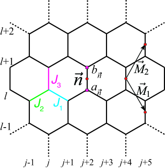
Figure 1: Schematic representation of the Kitaev model on a honeycomb lattice. The bonds $J_{1}$, $J_{2}$ and $J_{3}$ shows nearest neighbor couplings between $x$, $y$ and $z$ components of the spins respectively. $\vec{n}$ represents the position vector of the midpoint of each vertical bond (unit cell). The vectors $\vec{M}_{1}$ and $\vec{M}_{2}$ are spanning vectors of the lattice. In the Fermionic representation of the model, the Majorana Fermions $a_{\vec{n}}$ and $b_{\vec{n}}$ sit at the bottom and top sites respectively of the vertical bond with center coordinate $\vec{n}$ as shown.

We begin with the study of slow dynamics in the Kitaev model kitaev1 ; sengupta1 . The Hamiltonian for this model, schematically represented in Fig. 1, is given by

$$H_{K} = \sum_{j+l={\rm even}}(J_{1}\tau_{j,l}^{x}\tau_{j+1,l}^{x}+J_{2}\tau_{j-1,l}^{y}\tau_{j,l}^{y}+J_{3}\tau_{j,l}^{z}\tau_{j,l+1}^{z}),$$

where $\vec{\tau}_{jl}=(\tau_{jl}^{x},\tau_{jl}^{y},\tau_{jl}^{z})$ denote Pauli matrices at the site $(j,l)$ of the honeycomb lattice, $J_{1}$, $J_{2}$, and $J_{3}$ represent nearest-neighbor couplings between $x$, $y$ and $z$ components of the spins respectively. It is well-known that $H_{K}$ can be represented in terms of Fermionic fields by a straightforward Majorana transformation: $a_{jl}=\left(\prod_{i=-\infty}^{j-1}~{}\tau_{il}^{z}\right)~{}\tau_{jl}^{y}~{}~{}{\rm for}~{}{\rm~{}even}~{}j+l$ and $b_{jl}=\left(\prod_{i=-\infty}^{j-1}~{}\tau_{il}^{z}\right)~{}\tau_{jl}^{x}~{}~{}{\rm for}~{}{\rm~{}odd}~{}j+l$ sengupta1 . This leads to the Fermionic Hamiltonian

$$H_{F} = i~{}\sum_{\vec{n}}~{}[J_{1}~{}b_{\vec{n}}a_{{\vec{n}}-{\vec{M}}_{1}}~{}+~{}J_{2}~{}b_{\vec{n}}a_{{\vec{n}}+{\vec{M}}_{2}}$$ (3)

$$+J_{3}D_{\vec{n}}~{}b_{\vec{n}}a_{\vec{n}}],$$

where $\vec{n}={\sqrt{3}}{\hat{i}}~{}n_{1}+(\frac{\sqrt{3}}{2}{\hat{i}}+\frac{3}{2}{\hat{j}})~{}n_{2}$ denote the midpoints of the vertical bonds. Here $n_{1},n_{2}$ run over all integers so that the vectors $\vec{n}$ form a triangular lattice whose vertices lie at the centers of the vertical bonds of the underlying honeycomb lattice. The Majorana Fermions $a_{\vec{n}}$ and $b_{\vec{n}}$ sit at the bottom and top sites respectively of the bond labeled $\vec{n}$. The vectors ${\vec{M}}_{1}=\frac{\sqrt{3}}{2}{\hat{i}}-\frac{3}{2}{\hat{j}}$ and ${\vec{M}}_{2}=\frac{\sqrt{3}}{2}{\hat{i}}+\frac{3}{2}{\hat{j}}$ are spanning vectors for the lattice, and $D_{\vec{n}}$ can take the values $\pm 1$ independently for each $\vec{n}$. The crucial point that makes the solution of Kitaev model feasible is that $D_{\vec{n}}$ commutes with $H_{F}$, so that all the eigenstates of $H_{F}$ can be labeled by specific values of $D_{\vec{n}}$. It is well-known that the ground state of the model corresponds to $D_{\vec{n}}=1$ on all links kitaev1 .

For $D_{\vec{n}}=1$, Eq. (3) can be diagonalized as

$$H_{F}=\sum_{\vec{k}}\psi_{\vec{k}}^{\dagger}H_{\vec{k}}\psi_{\vec{k}},$$ (4)

where $\psi_{\vec{k}}^{\dagger}=(a_{\vec{k}}^{\dagger},~{}b_{\vec{k}}^{\dagger})$ are Fourier transforms of $a_{\vec{n}}$ and $b_{\vec{n}}$, the sum over $\vec{k}$ extends over half the Brillouin zone (BZ) of the triangular lattice formed by the vectors $\vec{n}$, and $H_{\vec{k}}$ can be expressed in terms of the Pauli matrices $\sigma^{i}$ in particle-hole space as

$$H_{\vec{k}} = 2[J_{1}\sin({\vec{k}}\cdot{\vec{M}}_{1})-J_{2}\sin({\vec{k}}\cdot{\vec{M}}_{2})]\sigma^{1}$$ (5)

$$+2[J_{3}+J_{1}\cos({\vec{k}}\cdot{\vec{M}}_{1})+J_{2}\cos({\vec{k}}\cdot{\vec{M}}_{2})]\sigma^{2}.$$

The spectrum consists of two bands with energies $E_{\vec{k}}^{\pm}=\pm E_{\vec{k}}$ sengupta1 , where

$$E_{\vec{k}} = 2[\{J_{1}\sin({\vec{k}}\cdot{\vec{M}}_{1})-J_{2}\sin({\vec{k}}\cdot{\vec{M}}_{2})\}^{2}$$ (6)

$$+\{J_{3}+J_{1}\cos({\vec{k}}\cdot{\vec{M}}_{1})+J_{2}\cos({\vec{k}}\cdot{\vec{M}}_{2})\}^{2}]^{1/2}.$$

For $|J_{1}-J_{2}|\leq J_{3}\leq J_{1}+J_{2}$, the bands touch each other, and the energy gap $\Delta_{\vec{k}}=E_{\vec{k}}^{+}-E_{\vec{k}}^{-}$ vanishes for special values of $\vec{k}$ leading to a gapless phase. In particular we note that for $J_{1}=J_{2}=1$ and $J_{3}=2$, the gap vanishes at $\vec{k}_{c}=(2\pi/\sqrt{3},0)$ and around this point $\Delta_{\vec{k}}\sim k_{y}$ and $\Delta_{\vec{k}}\sim k_{x}^{2}$. Thus this critical point constitutes an example of an anisotropic critical point with $z=m=1$ and $d=z^{\prime}=2$. We note that such an anisotropic scaling occurs for any non-zero value of $J_{1}$ and $J_{2}$ at $J_{3}=(J_{1}+J_{2})$.

We now consider a dynamics in this model $J_{3}(t)=(J_{1}+J_{2}-Jt/\tau)$ from $t=-\infty$ to $t=0$ at a fixed rate $1/\tau$ which brings the system from a gapped phase to the anisotropic critical point at $\vec{k}_{c}$. Although this quench problem can be solved for any $J_{1}$ and $J_{2}$, we shall fix $J_{1}=J_{2}=J$ for simplicity and scale all energies (times) by $J$ ($\hbar/J$) in the subsequent analysis. This choice does not change the scaling properties which we seek. Also, to study the time evolution of the system, we note that after an unitary transformation $U=\exp(-i\sigma^{1}\pi/4)$, we obtain $H_{F}=\sum_{\vec{k}}\psi_{\vec{k}}^{{}^{\prime}\dagger}H^{\prime}_{\vec{k}}\psi^{\prime}_{\vec{k}}$, where $H^{\prime}_{\vec{k}}=UH_{\vec{k}}U^{\dagger}$ is given by

$$H^{\prime}_{\vec{k}}=2[(g_{\vec{k}}-t/\tau)\sigma^{3}+\alpha_{\vec{k}}\sigma^{1}],$$ (7)

where $\alpha_{\vec{k}}=\sin({\vec{k}}\cdot{\vec{M}}_{1})-\sin({\vec{k}}\cdot{\vec{M}}_{2})$ and $g_{\vec{k}}=2+\cos({\vec{k}}\cdot{\vec{M}}_{1})+\cos({\vec{k}}\cdot{\vec{M}}_{2})$. Hence the off-diagonal elements of $H^{\prime}_{\vec{k}}$ remain time independent, and the quench problem reduces to a Landau-Zener problem for each $\vec{k}$.

The state of the system after the quench at $t=0$ can be found by solving the Landau-Zener problem at each $\vec{k}$ with the initial condition $\psi_{\vec{k}}^{G}(t=-\infty)=|1\rangle=(0,1)^{T}$ for all $\vec{k}$. After some algebra, one obtains for a given $\vec{k}$ and at $t=0$ lzpapers1

$$|\psi_{\vec{k}}\rangle^{d} = e^{-\pi\alpha_{\vec{k}}^{2}\tau/4}\Big{(}e^{3i\pi/4}D_{\mu_{\vec{k}}}(\nu_{\vec{k}})|1\rangle$$ (8)

$$+\alpha_{\vec{k}}\sqrt{\tau}D_{\mu_{\vec{k}}-1}(\nu_{\vec{k}})|0\rangle\Big{)},$$

where $\nu_{\vec{k}}=2ig_{\vec{k}}\sqrt{\tau}\exp(-i\pi/4)$, $\mu_{\vec{k}}=-i\alpha_{\vec{k}}^{2}\tau$ and $D_{\mu}$ are parabolic cylinder functions. The excited state at $t=0$, solved by diagonalizing $H^{\prime}_{\vec{k}}(t=0)$, yields, for a given $\vec{k}$, $|\psi_{\vec{k}}^{+}\rangle=((E_{\vec{k}}^{+}-2g_{\vec{k}})|1\rangle+2\alpha_{\vec{k}}|0\rangle)/{\mathcal{D}}_{\vec{k}}$, where ${\mathcal{D}}_{\vec{k}}=[(E_{\vec{k}}^{+}-2g_{\vec{k}})^{2}+4\alpha_{\vec{k}}^{2}]^{1/2}$. Thus the probability of defect formation, given by $p_{\vec{k}}=|\langle\psi_{\vec{k}}^{+}|\psi_{\vec{k}}\rangle^{d}|^{2}$, can be obtained as

$$p_{\vec{k}} = \frac{4\alpha^{2}_{\vec{k}}e^{-\pi\alpha_{\vec{k}}^{2}\tau/2}}{{\mathcal{D}}_{\vec{k}}^{2}}\Big{|}\alpha_{\vec{k}}\sqrt{\tau}D_{\mu_{\vec{k}}-1}(\nu_{\vec{k}})+\frac{E_{\vec{k}}^{+}-2g_{\vec{k}}}{2\alpha_{\vec{k}}}$$ (9)

$$\times e^{-3i\pi/4}D_{\mu_{\vec{k}}}(\nu_{\vec{k}})\Big{|}^{2}.$$

Since $\tau$ is large for slow dynamics, the contribution to the defect formation comes from a small region near the critical point where $\Delta_{\vec{k}}$ is sufficiently small for $\vec{k}\simeq\vec{k}_{c}$. The density of defects can be thus estimated by expanding $p_{\vec{k}}$ about $\vec{k}=\vec{k}_{c}$: $n\simeq\int d\delta k_{x}\,d\delta k_{y}\,p_{\vec{k}=\vec{k}_{c}+\vec{\delta k}}$, where the limits of integration can now be safely extended to infinity. To compute this integral, we note that around $\vec{k}=\vec{k}_{c}$, $\alpha_{\vec{\delta k}}\simeq 3\delta k_{y}$ and $g_{\vec{\delta k}}\sim 3(\delta k_{x}^{2}+3\delta k_{y}^{2})/4$. Thus a redefinition of variables $\delta k_{x}\to\delta k^{\prime}_{x}=\delta k_{x}\tau^{1/4}$ and $\delta k_{y}\to\delta k^{\prime}_{y}=\delta k_{y}\tau^{1/2}$ allows us to extract the $\tau$ dependence of the defect density

$$n\simeq\int d\delta k_{x}\,d\delta k_{y}\,p_{\vec{\delta k}},\,\sim\tau^{-3/4}\int d\delta k^{\prime}_{x}\,d\delta k^{\prime}_{y}\,p_{\vec{\delta k^{\prime}}}.$$ (10)

A similar analysis can be carried out for computation of residual energy $Q=(2\pi)^{-2}\int d^{2}kp_{\vec{k}}\Delta_{\vec{k}}$. Here we note that near the critical point $\vec{k}=\vec{k}_{c}$, $\Delta_{\vec{k}}\simeq 4\sqrt{9\delta k_{y}^{2}+9(\delta k_{x}^{2}+3\delta k_{y}^{2})^{2}/16}$ and thus scale as $\tau^{-1/2}$. Thus one obtains

$$Q\simeq\int d\delta k_{x}\,d\delta k_{y}\,\Delta_{\vec{\delta k}}p_{\vec{\delta k}},\,\sim\tau^{-5/4}\int d\delta k^{\prime}_{x}\,d\delta k^{\prime}_{y}\,\Delta_{\vec{\delta k^{\prime}}}p_{\vec{\delta k^{\prime}}}.$$

Eqs. (10) and (II) show that $n\sim\tau^{-3/4}$ and $Q\sim\tau^{-5/4}$ at the critical point. These scaling laws do not conform to the predictions of earlier works on defect production during passage through isotropic quantum critical points pol2 or critical surfaces sengupta1 ; their origin lies in the anisotropic scaling of $\delta k_{x}$ and $\delta k_{y}$ with the quench time $\tau$.

To generalize these results for arbitrary $d$-dimensional anisotropic critical points, where the energy gap $\Delta_{\vec{k}}\sim k_{i}^{z}$ for $m$ directions and $\sim k_{i}^{z^{\prime}}$ for $d-m$ directions, we provide a simple phase space argument as first proposed in Ref. zurek1, . We consider a general power-law quench with $\lambda(t)=\lambda_{0}|t/\tau|^{\alpha}{\rm Sgn}(t)$ which starts at $t=-\infty$ and reaches the critical point at $t=0$. We first note that the adiabaticity condition breaks down when the rate of change of the energy gap become equivalent to the square of the gap: $d\Delta_{\vec{k}}/dt\geq\Delta_{\vec{k}}^{2}$. Since $\Delta_{\vec{k}}\sim\lambda^{z\nu}|t/\tau|^{z\nu\alpha}$, we find that the time spent by the system in the non-adiabatic regime is given by $\hat{t}\sim\tau^{z\nu\alpha/(z\nu\alpha+1)}$. The scaling of the energy gap in this regime can thus be written as $\Delta_{\vec{k}}\sim\tau^{-z\nu\alpha/(z\nu\alpha+1)}$. The phase space for defect production is given by $\Omega_{n}\sim k_{1}..k_{d}$. Since $\Delta_{\vec{k}}\sim k_{i}^{z}$ for $i=1..m$ and $k_{i}^{z^{\prime}}$ for $i=m+1..d$, we finally obtain

$$n\sim\tau^{-(m+(d-m)z/z^{\prime})\nu\alpha/(z\nu\alpha+1)}.$$ (12)

A similar argument can also be presented for the residual energy. We note that for $z\leq z^{\prime}$, the leading behavior of the energy gap near the quantum critical point, where the defects are produced, is $\Delta_{\vec{k}}\sim k_{i}^{z}$ for $1\leq i\leq m$. Thus the phase space for the residual energy production is $\Omega_{Q}\sim\Delta_{\vec{k}}k_{1}..k_{d}$ leading to a scaling of $Q$ as

$$Q\sim\tau^{-[(m+z)+(d-m)z/z^{\prime}]\nu\alpha/(z\nu\alpha+1)}.$$ (13)

We note that the scaling laws, Eqs. (12) and (13), reproduce their isotropic counterparts for $z=z^{\prime}$ leading to $n\sim\tau^{-d\nu\alpha/(z\nu\alpha+1)}$ and $Q\sim\tau^{-(d+z)\nu\alpha/(z\nu\alpha+1)}$ sen1 ; pol2 ; pol3 . Also, the scaling of the Kitaev model for linear time evolution elaborated in this work is reproduced for $d=z^{\prime}=2$, and $z=\nu=\alpha=1$ leading $n\sim\tau^{-3/4}$ and $Q\sim\tau^{-5/4}$. Moreover, we note that the scaling of defect density for a linear quench through a gapless surface can also be obtained from Eq. (12) by noting that for such quenches the energy gap depends only on the $m$ momenta components orthogonal to the $d-m$ dimensional gapless surface. This can be represented by putting $z^{\prime}\to\infty$ (since $k_{\parallel}\sim\Delta_{\vec{k}}^{1/z^{\prime}}$) leading to the scaling law $n\sim\tau^{-m\nu/(z\nu+1)}$ sengupta1 . Thus Eqs. (12) and (13) reproduce all earlier results on defect production for slow dynamics across quantum critical lines and surfaces as special cases. Finally, we would like to point out that the maximum values of these exponents is $2$ which can be obtained by similar considerations as in the cases of isotropic critical points pol3 .

To verify these scaling laws, we now study non-linear power-law dynamics in the Kitaev model numerically. To this end, we again restrict ourselves to $J_{1}=J_{2}=1$ and evolve $J_{3}(t)=(2-|t/\tau|^{\alpha}{\rm Sgn}(t))$ for $-\infty\leq t\leq 0$ so that the anisotropic critical point is reached at $t=0$. The corresponding time-dependent Hamiltonian is given by $H(\vec{k};t)=\sum_{\vec{k}}\psi_{\vec{k}}^{\dagger}\left[(g_{\vec{k}}-|t/\tau|^{\alpha}{\rm Sgn}(t))\sigma^{3}+\alpha_{\vec{k}}\sigma^{1}\right]\psi_{\vec{k}}$. We solve the time-dependent Schrödinger equation $i\partial_{t}\psi_{\vec{k}}=H(\vec{k};t)\psi(\vec{k})$ numerically for each $k$, compute $p_{\vec{k}}$, and use it to obtain the defect density $n=\int d^{2}kp_{\vec{k}}$ and $Q=\int d^{2}k\Delta_{\vec{k}}p_{\vec{k}}$ numerically as a function of $\tau$ and $\alpha$. 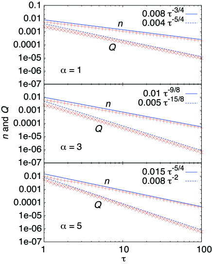The plots of $n$ and $Q$ vs $\tau$ are shown in Fig. 2 for several representative values of $\alpha$. The lines in the figure indicate the power laws expected from Eqs. 12 and 13 ($n\sim\tau^{-3\alpha/[2(\alpha+1)]}$ and $Q\sim\tau^{-5\alpha/[2(\alpha+1)]}$) for $d=z^{\prime}=2$ and $z=\nu=m=1$. The agreement between the numerical and theoretical results corroborates the scaling theory proposed in this work.

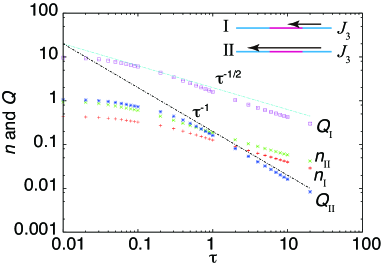
Figure 2: Numerical results on the defect density $n$ and residual energy $Q$. The time-dependent Schrödinger equation is solved in the momentum space for systems with size up to $512\times 512$ unit cells. The parameter $\alpha$ specifying the evolution of $J_{3}=2-|t/\tau|^{\alpha}{\rm Sgn}(t)$ is chosen as $\alpha=1$, $3$ and $5$. The lines indicate the power laws expected from Eqs. (12) and (13) for $d=z^{\prime}=2$ and $z=\nu=m=1$, $n\sim\tau^{-3\alpha/[2(\alpha+1)]}$ and $Q\sim\tau^{-5\alpha/[2(\alpha+1)]}$. The agreement between curves obtained numerically and the corresponding power laws is remarkable. In all plots, $t$ varies from an initial value $t_{\rm in}=-3\tau$ to a final value $t_{\rm f}=0$.

III Correlation function

In this section, we compute the independent correlation function for the Kitaev model for linear time evolution. Since the model can be represented by free Fermions, it is easy to see that the only non-zero independent correlators are those between free Fermions which are given by

$$\langle O_{\vec{r}}\rangle = i\langle b_{\vec{n}}a_{\vec{n}+\vec{r}}\rangle$$ (14)

$$= \frac{4i}{N_{s}}\sum_{\vec{k}}[\langle b_{\vec{k}}^{\dagger}a_{\vec{k}}\rangle\exp(i\vec{k}\cdot\vec{r})-{\rm h.c.}],$$

where $\langle..\rangle$ denotes expectation value with respect to a direct product of states involving $\vec{k}$ only, ${\rm h.c.}$ denotes hermitian conjugate, and $N_{s}$ is the number of sites. After an unitary transformation $U=\exp(-i\sigma^{1}\pi/4)$, we find

$$\langle O_{\vec{r}}\rangle=-\frac{2}{N}\sum_{\vec{k}}\langle\psi_{\vec{k}}^{{}^{\prime}\dagger}[-\cos(\vec{k}\cdot\vec{r})\sigma^{3}+\sin(\vec{k}\cdot\vec{r})\sigma^{1}]\psi^{\prime}_{\vec{k}}\rangle.$$ (15)

The interpretation of these correlation functions in terms of the original spin degrees of freedom have already been pointed out in Ref. sengupta1, . For $\vec{r}=0$, $\langle O_{\vec{r}}\rangle$ represents correlations between $z$ components between spins at the end of the vertical bond whose midpoint is denoted by $\vec{n}$. For ${\vec{r}}\neq 0$, it represents correlation between product of multiple spin operators which begins with $\tau^{x}$ or $\tau^{y}$ on a $b$ or $a$ site at $\vec{n}=(j,l)$ and ends with $\tau^{x}$ or $\tau^{y}$ on an $a$ or $b$ site at $\vec{n}+\vec{r}=(j^{\prime},l^{\prime})$ with a string of $\tau^{z}$ operators living on sites in between. Note that the Fermionic representation in terms of free Fermions with $D_{\vec{n}}=1$ ensures that these multispin correlation functions are the only non-zero independent spin correlation functions of the model.

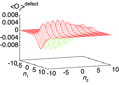
Figure 3: Plot of the correlation function $\langle O_{\vec{r}}\rangle^{defect}$ as a function of $n_{1}$ and $n_{2}$ for linear quench of $J_{3}/J_{1}$ from $5$ to $2$ with $J_{1}=J_{2}=1$ and $\tau=5$.

The ground state with a fixed $\vec{k}$ for $J_{3}=2$ is given by $|\psi_{\vec{k}}^{-}\rangle=((E_{\vec{k}}^{-}-2g_{\vec{k}})|1\rangle+2\alpha_{\vec{k}}|0\rangle)/{\mathcal{D}}_{\vec{k}}^{-}$, where ${\mathcal{D}}_{\vec{k}}^{-}=[(E_{\vec{k}}^{-}-2g_{\vec{k}})^{2}+4\alpha_{\vec{k}}^{2}]^{1/2}$. Noting that $|0\rangle$ and $|1\rangle$ are basis of $\psi^{\prime}_{\vec{k}}$, one finds, from Eq. (15), the correlation function of the ground state as

$$\langle O_{\vec{r}}\rangle^{G} = -\delta_{\vec{r0}}+\frac{1}{A}\int d^{2}k\left[2\frac{4\alpha_{\vec{k}}^{2}}{({\mathcal{D}}_{\vec{k}}^{-})^{2}}\cos(\vec{k}\cdot\vec{r})\right.$$ (16)

$$-\left.2\frac{2\alpha_{\vec{k}}(E_{\vec{k}}^{-}-2g_{\vec{k}})}{({\mathcal{D}}_{\vec{k}}^{-})^{2}}\sin(\vec{k}\cdot\vec{r})\right],$$

where $A=4\pi/3\sqrt{3}$ is the area of half of the Brillouin zone. As for the state after quench, a straightforward calculation using Eq. (8) shows

$$\langle O_{\vec{r}}\rangle^{d} = -\delta_{\vec{r}0}+\frac{1}{A}\int d^{2}ke^{-\pi\alpha_{\vec{k}}^{2}\tau/2}\alpha_{\vec{k}}\sqrt{\tau}\Big{[}2\alpha_{\vec{k}}\sqrt{\tau}$$ (17)

$$\times|D_{\mu_{\vec{k}}-1}(\nu_{\vec{k}})|^{2}\cos(\vec{k}\cdot\vec{r})-\Big{\{}e^{i3\pi/4}D^{\ast}_{\mu_{\vec{k}}-1}(\nu_{\vec{k}})$$

$$\times D_{\mu_{\vec{k}}}(\nu_{\vec{k}})+{\rm c.c.}\Big{\}}\sin(\vec{k}\cdot\vec{r})\Big{]}.$$

Note that $\langle O_{\vec{r}}\rangle^{d}$ reduces to $\langle O_{\vec{r}}\rangle^{G}$ with $\tau\to\infty$. The correlation between defects induced by non-adiabatic quench dynamics can be captured by the deviation of $\langle O_{\vec{r}}\rangle^{d}$ from $\langle O_{\vec{r}}\rangle^{G}$. Thus we define the defect correlation function by

$$\langle O_{\vec{r}}\rangle^{\rm defect}=\langle O_{\vec{r}}\rangle^{d}-\langle O_{\vec{r}}\rangle^{G}.$$ (18)

The nature of the spatial dependence of the defect correlation function for slow dynamics (large $\tau$) can be qualitatively understood for $J_{1}=J_{2}$ from Eq. (17). To this end, we first separate the contribution to $\langle O_{\vec{r}}\rangle^{d}$ which comes from around $\alpha_{\vec{k}}\simeq 1/\tau$ from those coming from other regions in the $\vec{k}$-space. For estimating the latter contribution, we consider $\tau\gg 1$ so that for $\alpha_{\vec{k}},g_{\vec{k}}\neq 0$, $|\mu_{\vec{k}}|,|\nu_{\vec{k}}|\to\infty$. We then note that the following identities for $D$ holds in the limit $b\to\infty$ with arbitrary ratio $a/b$

$$e^{-\pi b^{2}/4}D_{-ib^{2}-1}(ae^{i\pi/4})\simeq\sin(\theta)e^{-i(\eta+\pi/4)}/b,$$

$$e^{-\pi b^{2}/4}D_{-ib^{2}}(ae^{i\pi/4})\simeq\cos(\theta)e^{-i\eta},$$ (19)

where $\theta$ and $\eta$ are defined through the relations

$$\cos(\theta)(\sin(\theta)) = \sqrt{[1+(-)a/(2\sqrt{b^{2}+a^{2}/4})]/2},$$

$$\eta = -b^{2}/2+b^{2}\ln(a/2+\sqrt{b^{2}+a^{2}/4})$$ (20)

$$+a\sqrt{b^{2}+a^{2}/4}/2.$$

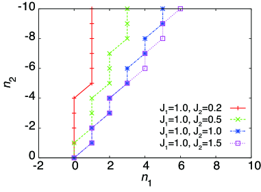
Figure 4: Plot of the peak positions of $\langle O_{\vec{r}}\rangle^{defect}$ in the $n_{1}-n_{2}$ plane for $J_{1}=1$ and several representative values of $J_{2}$. For each of these cases, the quench starts at $J_{3}/J_{1}=5$ and ends at the anisotropic critical point. Note that the axis of $n_{2}$ is upside down.

Identifying $b=\alpha_{\vec{k}}\sqrt{\tau}$ and $a=2g_{\vec{k}}\tau$ and substituting Eqs. (19) and (20) in Eq. (17), we find, after some straightforward algebra, that the integrand of Eq. (17) reduces to that of Eq. (16) for all $\vec{k}$ except those for which $\alpha_{\vec{k}}\sqrt{\tau}\simeq 1$. Thus, one finds that in this limit, the main contribution to $\langle O_{\vec{r}}\rangle^{\rm defect}$ comes from around the line $\alpha_{\vec{k}}\simeq 1/\sqrt{\tau}$. For large $\tau$, this is infinitesimally close to the line $\sin(\vec{k}\cdot\vec{M}_{1})=\sin(\vec{k}\cdot\vec{M}_{2})$. In this region of $k$ space, $|D_{\mu_{\vec{k}}-1}(\nu_{\vec{k}})|^{2}\simeq|D_{i-1}(\nu_{\vec{k}})|^{2}$ which, for large $\tau$ and $J_{3}=2$, is a sharply peaked function for $g_{\vec{k}}\simeq 0$ which occurs at $\vec{k}=\vec{k}_{c}$. Also, for $\vec{k}\simeq\vec{k}_{c}$, it can be easily checked that $[D^{\ast}_{\mu_{\vec{k}}-1}(\nu_{\vec{k}})D_{\mu_{\vec{k}}}(\nu_{\vec{k}})+{\rm h.c.}]\ll|D_{\mu_{\vec{k}}-1}(\nu_{\vec{k}})|^{2}$, so that the major contribution to $\langle O_{\vec{r}}\rangle^{\rm defect}$ comes from the coefficient of the $\cos(\vec{k}\cdot\vec{r})$ in the integrand. Using these observations and expressing $\vec{r}=(\sqrt{3}(n_{1}+n_{2}/2),3n_{2}/2)$, one can estimate the spatial dependence of the correlation function in the same line as in Ref. sengupta1, . In particular, the maxima of the correlation function is expected to occur along the maxima of $\cos(\vec{k}_{c}\cdot\vec{r})$ i.e. along the line $n_{1}+n_{2}/2=0$ in the $n_{1}-n_{2}$ plane. Away from this line, as shown in Ref. sengupta1, , $\langle O_{\vec{r}}\rangle^{\rm defect}$ is expected to decay exponentially as a function of $r$ with a characteristic decay length $\sim\sqrt{\tau}$.

A plot of $\langle O_{\vec{r}}\rangle^{\rm defect}$ as a function of $n_{1}$ and $n_{2}$, obtained by numerical evaluation of Eq. (18) are shown in Fig. 3 for $J_{1}=J_{2}=1$, corroborates the above-mentioned discussion. We find that $\langle O_{\vec{r}}\rangle^{\rm defect}$ peaks along the $n_{1}=-n_{2}/2$ line and decays to zero as we move away from this line. The decay length in the $n_{1}-n_{2}$ depends on $\tau$; for larger $\tau$ we have a sharper decay. The slope of the line along which $\langle O_{\vec{r}}\rangle^{\rm defect}$ peaks in the $n_{1}-n_{2}$ plane changes with $J_{1}/J_{2}$ since ${\vec{k}}_{c}$ depends on this ratio. This can be seen from Fig. 4 which plots the position of the peaks of the correlation functions for several representative values of $J_{1}/J_{2}$. The analysis of the preceding paragraph can be easily extended to these cases in the same line as in Ref. sengupta1, and is found to match the numerical results for all $J_{1}/J_{2}$.

IV Disordered Kitaev model

In this section, we study the dynamics of Kitaev model given by Eq. (4) with a random configuration of $D_{\vec{n}}$, namely for random assignment of values $\pm 1$ to the link variables $D_{\vec{n}}$. The dynamics is incorporated in the form of a power-law evolution of $J_{3}$ as in Sec. II.

The Hamiltonian (Eq. (3)) can be expressed using the real-space Fermion operators $\alpha_{\vec{n}}=\frac{1}{2}(b_{\vec{n}}-ia_{\vec{n}})$ at position $\vec{n}$ as

$$H_{F} = \sum_{\vec{n}}J_{1}\left(\alpha_{\vec{n}}+\alpha_{\vec{n}}^{\dagger}\right)\left(\alpha_{\vec{n}-\vec{M}_{1}}-\alpha_{\vec{n}-\vec{M}_{1}}^{\dagger}\right)$$ (21)

$$+J_{2}\left(\alpha_{\vec{n}}+\alpha_{\vec{n}}^{\dagger}\right)\left(\alpha_{\vec{n}+\vec{M}_{2}}-\alpha_{\vec{n}+\vec{M}_{2}}^{\dagger}\right)$$

$$+J_{3}D_{\vec{n}}(1-2\alpha_{\vec{n}}^{\dagger}\alpha_{\vec{n}}).$$

The first two terms represent hopping and pair-creation and annihilation of the Fermions while the third term induces a random local potential. For $J_{3}\gg J_{1,2}$, the third term dominates and the ground state of the system is composed of localized states of the Fermion. In contrast for $J_{3}=0$, the ground state is clearly delocalized. We now show numerically that a quantum phase transition takes place in between these two limits at $J_{3}=J_{3,c}$. Note that the existence of a sharp transition in the presence of the disorder is consistent with the Harris criteria $\nu d\geq 2$ since for the Kitaev model $d=2$ and $\nu=1$.

The Hamiltonian, Eq. (21), is written in a quadratic form as $H=\psi^{\dagger}M\psi$ with $\psi^{\dagger}=(\alpha_{\vec{n}_{1}}^{\dagger},\alpha_{\vec{n}_{2}}^{\dagger},\cdots,\alpha_{\vec{n}_{N}}^{\dagger},\alpha_{\vec{n}_{1}},\alpha_{\vec{n}_{2}},\cdots,\alpha_{\vec{n}_{N}})$, where $N$ is the number of vertical bonds (unit cells) in the system, and $M$ is a $2N\times 2N$ matrix given by

$$M=\frac{1}{2}\left[\begin{array}[]{@{\,}cc@{\,}}A&B\\ B^{\rm T}&-A\end{array}\right],$$ (22)

with

$$A_{\vec{n}_{i}-\vec{M}_{1},\vec{n}_{i}} = A_{\vec{n}_{i},\vec{n}_{i}-\vec{M}_{1}}=-J_{1},$$

$$A_{\vec{n}_{i}+\vec{M}_{2},\vec{n}_{i}} = A_{\vec{n}_{i},\vec{n}_{i}+\vec{M}_{2}}=-J_{2},$$

$$A_{\vec{n}_{i},\vec{n}_{i}} = 2J_{3}D_{\vec{n}_{i}},$$

$$B_{\vec{n}_{i}-\vec{M}_{1},\vec{n}_{i}} = -B_{\vec{n}_{i},\vec{n}_{i}-\vec{M}_{1}}=-J_{1},$$

$$B_{\vec{n}_{i}+\vec{M}_{2},\vec{n}_{i}}=-J_{2} = -B_{\vec{n}_{i},\vec{n}_{i}+\vec{M}_{2}}.$$ (23)

All other elements of $A$ and $B$ are zero. The matrix $M$ is diagonalized by a unitary matrix,

$$U=\left[\begin{array}[]{@{\,}cc@{\,}}u&v^{\ast}\\ v&u^{\ast}\end{array}\right],$$ (24)

as $U^{\dagger}MU=D$, where $D$ is a diagonal matrix. We note that the form of $M$ necessitates that if $\epsilon_{\mu}$ is an eigenvalue of $M$, so is $-\epsilon_{\mu}$. We hereafter suppose $\epsilon_{\mu}>0$ and choose $U$ so that $\epsilon_{\mu}$ ($\mu=1,2,\cdots,N$) enter upper half diagonal elements of $D$. Defining a fermion operator as

$$\gamma_{\mu}=\sum_{\vec{n}}u^{\ast}_{\vec{n},\mu}\alpha_{\vec{n}}+v^{\ast}_{\vec{n},\mu}\alpha^{\dagger}_{\vec{n}},$$ (25)

the diagonalized Hamiltonian is written as

$$H_{F}=\sum_{\mu=1}^{N}\epsilon_{\mu}(2\gamma^{\dagger}_{\mu}\gamma_{\mu}-1).$$ (26)

The ground-state energy is given by $E_{g}=-\sum_{\mu=1}^{N}\epsilon_{\mu}$. The energy gap from the ground state to the first excited state is thus given by $\Delta=2\epsilon_{1}$ where $\epsilon_{1}$ is the smallest positive eigenvalue.

With this observation, we now compute the gap $\Delta$ numerically for finite sizes and obtain the distribution of gaps by changing the configuration of $\{D_{\vec{n}}\}$.

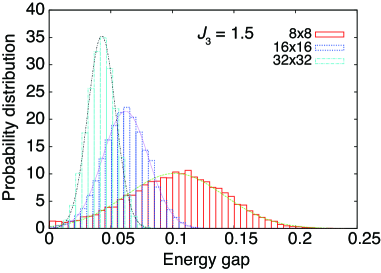
Figure 5: Probability distribution of excitation gaps at $J_{3}=1.5$. $10000$ instances of $\{D_{\vec{n}}\}$ are generated and for each of them we obtained the excitation gap $2\epsilon_{1}$ by numerically diagonalizing the matrix $M$.

We find that the property of the distribution of gaps is qualitatively different for $J_{3}\mathrel{\mathchoice{\lower 2.58334pt\vbox{\halign{$\m@th\displaystyle\hfil#\hfil$\cr<\crcr\sim\crcr}}}{\lower 2.58334pt\vbox{\halign{$\m@th\textstyle\hfil#\hfil$\cr<\crcr\sim\crcr}}}{\lower 2.58334pt\vbox{\halign{$\m@th\scriptstyle\hfil#\hfil$\cr<\crcr\sim\crcr}}}{\lower 2.58334pt\vbox{\halign{$\m@th\scriptscriptstyle\hfil#\hfil$\cr<\crcr\sim\crcr}}}}1.5$ and $J_{3}\mathrel{\mathchoice{\lower 2.58334pt\vbox{\halign{$\m@th\displaystyle\hfil#\hfil$\cr>\crcr\sim\crcr}}}{\lower 2.58334pt\vbox{\halign{$\m@th\textstyle\hfil#\hfil$\cr>\crcr\sim\crcr}}}{\lower 2.58334pt\vbox{\halign{$\m@th\scriptstyle\hfil#\hfil$\cr>\crcr\sim\crcr}}}{\lower 2.58334pt\vbox{\halign{$\m@th\scriptscriptstyle\hfil#\hfil$\cr>\crcr\sim\crcr}}}}1.5$. Let us first consider the case with $J_{3}=1.5$ for which the distribution of the gaps is shown in Fig. 5 for several system sizes. The shown distribution allows a Gaussian fit: $N(\Delta)=(2\pi\sigma^{2})^{-1/2}e^{-(\Delta-\bar{\Delta})^{2}/2\sigma^{2}}$ using the average $\overline{\Delta}$ and the variance $\sigma^{2}=\overline{\Delta^{2}}-\overline{\Delta}^{2}$, where $\bar{}$ stands for the average over the random configuration of $\{D_{\vec{n}}\}$.

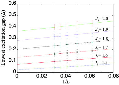
Figure 6: Finite size scaling of the average of gaps for $J_{3}=1.5$, $1.6$, $1.7$, $1.8$, $1.9$, and $2.0$. We find that the average of gaps is scaled by $1/L$, where $L$ is the length of the system ($N=L^{2}$).

Figure 6 shows the size scaling of $\bar{\Delta}$ for several $J_{3}\geq 1.5$. We find ${\bar{\Delta}}$ scales linearly with $1/L$. Since the variance of gaps tends to vanish for $L\to\infty$, one can estimate the gap in the thermodynamic limit $\Delta_{\infty}$ by extrapolating the fitting line of $\bar{\Delta}$ for $1/L\to 0$. Such a behavior of $\Delta_{\infty}$ is to be contrasted with that for $J_{3}=1$ as shown in Fig. 7. 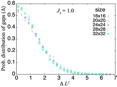For $J_{3}=1$, we find that the probability distribution of gaps scales as $\Delta\sim 1/L^{2}$ as seen from the collapse of the data for several system sizes (Fig. 7). 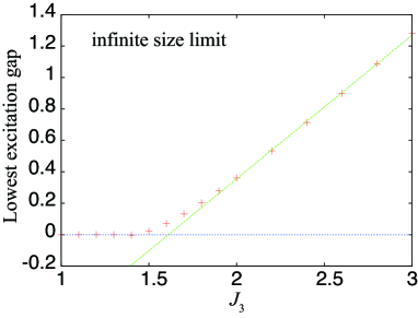The difference in behavior of ${\bar{\Delta}}$ can be further understood by plotting $\Delta_{\infty}$ for several values of $J_{3}$. This is shown in Fig. 8. We find that for $J_{3}\mathrel{\mathchoice{\lower 2.58334pt\vbox{\halign{$\m@th\displaystyle\hfil#\hfil$\cr<\crcr\sim\crcr}}}{\lower 2.58334pt\vbox{\halign{$\m@th\textstyle\hfil#\hfil$\cr<\crcr\sim\crcr}}}{\lower 2.58334pt\vbox{\halign{$\m@th\scriptstyle\hfil#\hfil$\cr<\crcr\sim\crcr}}}{\lower 2.58334pt\vbox{\halign{$\m@th\scriptscriptstyle\hfil#\hfil$\cr<\crcr\sim\crcr}}}}1.4$ the gap vanishes, while it increases linearly with $J_{3}$ for $J_{3}\geq 1.5$. The position of the critical point $J_{3,c}$ can therefore be estimated to be around $1.5$. Moreover, the gap $\Delta$ increases as $\Delta\propto|J_{3}-J_{3,c}|$ for $J_{3}\geq 1.5$ leading to $z\nu=1$ for the transition.

Having established the presence of a quantum critical point in the disordered Kitaev model, we now study the dynamical behavior during slow non-adiabatic linear time evolution $J_{3}(t)=-Jt/\tau$ which takes the system from a gapped region ($J_{3}=5$) either to a gapless region ($J_{3}=0$) or to a gapped region passing through the gapless region ($J_{3}=-5$). In order to obtain quantities of interest, we switch to the Heisenberg picture barouch ; caneva and introduce the time-evolution operator $U(t)$, $|\Psi(t)\rangle=U(t)|\Psi(t_{\rm in})\rangle$, where $t_{\rm in}$ denotes the initial time. The operator $\alpha_{\vec{n}}$ in the Heisenberg picture is denoted by $\alpha^{\rm H}_{\vec{n}}(t)=U^{\dagger}(t)\alpha_{\vec{n}}U(t)$. Computing the commutator of $\alpha_{\vec{n}}$ and $H_{F}$ expressed by Eq. (21), the Heisenberg equation of motion for $\alpha^{\rm H}_{\vec{m}}$ is given by

$$i\frac{d}{dt}\alpha^{\rm H}_{\vec{m}}(t)=\sum_{\vec{n}}\left(A_{\vec{m},\vec{n}}\alpha_{\vec{n}}^{\rm H}(t)+B_{\vec{m},\vec{n}}\alpha^{{\rm H}\dagger}_{\vec{n}}(t)\right).$$ (27)

Figure 7: The probability distribution of gaps at $J_{3}=1.0$. Horizontal axis is the excitation gap multiplied by $L^{2}$. The curves with different size almost collapse, meaning that the distribution of gaps is given by a function of $\Delta L^{2}$ and the gap vanishes as $1/L^{2}$ with increasing $L$.

We define matrices $u_{\vec{m},\nu}(t)$ and $v_{\vec{m},\nu}(t)$ by an expansion of $\alpha^{\rm H}_{\vec{m}}(t)$ by $\gamma_{\nu,{\rm in}}$, operators which diagonalize the Hamiltonian at initial time $t_{\rm in}$ (see Eq. (26)):

$$\alpha^{\rm H}_{\vec{m}}(t)=\sum_{\nu}\left(u_{\vec{m},\nu}(t)\gamma_{\nu,{\rm in}}+v^{\ast}_{\vec{m},\nu}(t)\gamma^{\dagger}_{\nu,{\rm in}}\right).$$ (28)

Substituting this expansion for $\alpha^{\rm H}$’s in Eq. (27), one obtains equations of motion for $u_{\vec{m},\nu}(t)$ and $v^{\ast}_{\vec{m},\nu}(t)$:

$$i\frac{d}{dt}u_{\vec{m},\nu}(t) = \sum_{\vec{n}}A_{\vec{m},\vec{n}}u_{\vec{n},\nu}(t)+B_{\vec{m},\vec{n}}v_{\vec{n},\nu}(t),$$ (29)

$$i\frac{d}{dt}v^{\ast}_{\vec{m},\nu}(t) = \sum_{\vec{n}}A_{\vec{m},\vec{n}}v^{\ast}_{\vec{n},\nu}(t)+B_{\vec{m},\vec{n}}u^{\ast}_{\vec{n},\nu}(t).$$ (30)

The initial conditions for $u_{\vec{m},\nu}(t)$ and $v_{\vec{m},\nu}(t)$ are written as $u_{\vec{m},\nu}(t_{\rm in})=u_{\vec{m},\nu,{\rm in}}$ and $v_{\vec{m},\nu}(t_{\rm in})=v_{\vec{m},\nu,{\rm in}}$, where $u_{\rm in}$ and $v_{\rm in}$ are block matrices of $U$ diagonalizing $M$ at initial time. To obtain the expressions of $n$ and $Q$ at final time $t_{\rm f}$, we introduce notations $u_{\rm f}$, $v_{\rm f}$, $\epsilon_{\mu,{\rm f}}$, and $\gamma_{\mu,{\rm f}}$ so that $H_{F}(t_{\rm f})=\sum_{\mu}\epsilon_{\mu,{\rm f}}(2\gamma^{\dagger}_{\mu,{\rm f}}\gamma_{\mu,{\rm f}}-1)$, where

$$\gamma_{\mu,{\rm f}}=\sum_{\vec{n}}u^{\ast}_{\vec{n},\mu,{\rm f}}\alpha_{\vec{n}}+v^{\ast}_{\vec{n},\mu,{\rm f}}\alpha^{\dagger}_{\vec{n}}.$$ (31)

The density of excitation $n$ and the residual energy $Q$ can now be defined by

$$n = \frac{1}{N}\sum_{\mu=1}^{N}\langle\Psi(t_{\rm f})|\gamma^{\dagger}_{\mu,{\rm f}}\gamma_{\mu,{\rm f}}|\Psi(t_{\rm f})\rangle,$$

$$Q = \langle\Psi(t_{\rm f})|H_{F}(t_{\rm f})|\Psi(t_{\rm f})\rangle-E_{g}.$$ (32)

Next, we switch to the Fermion operators $\alpha$ from $\gamma_{\rm f}$ using Eq. (31)and shift to the Heisenberg representation. Substituting the expansion Eq. (28) in Eq. (32), one obtains

$$n = \frac{1}{N}{\rm tr}\left[\left(v^{T}_{\rm f}u(t_{\rm f})+u^{T}_{\rm f}v(t_{\rm f})\right)\left(v^{\dagger}(t_{\rm f})u^{\ast}_{\rm f}+u^{\dagger}(t_{\rm f})v^{\ast}_{\rm f}\right)\right],$$

$$Q = 2\sum_{\mu=1}^{N}\epsilon_{\mu,{\rm f}}$$

$$\times\left[\left(v^{T}_{\rm f}u(t_{\rm f})+u^{T}_{\rm f}v(t_{\rm f})\right)\left(v^{\dagger}(t_{\rm f})u^{\ast}_{\rm f}+u^{\dagger}(t_{\rm f})v^{\ast}_{\rm f}\right)\right]_{\mu,\mu}.$$

First, we present numerical results for two cases of the quench. For each value of the quench time $\tau$, simulations were carried for $16$ different configurations of $\{D_{\vec{n}}\}$ for obtaining a large enough sample set for disorder averaging. Figure 9 shows the disorder averaged values of density of excitations and residual energy as a function of $\tau$ after the time evolution. The results of simulation suggest that for large $\tau$, the density of excitation $n$ and residual energy $Q$ scale with $\tau$ as

$$n \sim \tau^{-1/2},\quad Q\sim\tau^{-1},$$ (34)

for an evolution ending inside a gapless phase and

$$n \sim \tau^{-1/2},\quad Q\sim\tau^{-1/2},$$ (35)

for that ending in a gapped phase after passing through the gapless phase. We note that these scaling laws are different from those obtained for uniform $D_{\vec{n}}$ sen1 .

Figure 8: The excitation gap $\Delta$ in the thermodynamic limit estimated by the finite-size scaling. The gap vanishes for $J_{3}$ less than $J_{3}\sim 1.4$, while it increases with $J_{3}$ almost linearly for $J_{3}$ larger than $J_{3}\sim 1.5$. Although some ambiguity exists between $J_{3}\sim 1.4$ and $1.5$, the critical point lies around $J_{3,c}\simeq 1.5$. Since the gap increases as $\Delta\propto(J_{3}-J_{3,c})$, one should have $z\nu=1$.

Figure 9: Scalings of the density of excitations and residual energy after a quench of $J_{3}$ from $5$ to $-5$ and from $5$ to $0$. The density of excitations is scaled as $n_{ex}\sim\tau^{-1/2}$ in both cases. The scaling of residual energy is $Q\sim\tau^{-1}$ when $J_{3}$ stops at $5$ and $Q\sim\tau^{-1/2}$ when $J_{3}$ stops at $0$. Simulations are carried out for systems with $16\times 16$ unit cells. The average is taken over 16 configurations of $\{D_{\vec{n}}\}$.

A qualitative explanation of such scaling laws for $n$ and $Q$ can be obtained as follows. We recall that for dynamics in critical systems without disorder, the condition for diabaticity is given by $\frac{d\Delta}{dt}\geq\Delta^{2}$ (Ref. pol1, ). In generic second order quantum phase transition with critical exponents $z$ and $\nu$, one can write $\Delta\sim\lambda^{z\nu}$ where $\lambda$ is quenched with a rate $1/\tau$. This yields standard expressions pol1 $\hat{\Delta}\sim\tau^{-z\nu/(z\nu+1)}$. From this, one can estimate the scaling form of the density of excitations and the residual energies to be

$$n\sim\int_{0}^{\hat{\Delta}}D(\varepsilon)d\varepsilon,\quad Q\sim\int_{0}^{\hat{\Delta}}(\Delta_{\rm f}+\varepsilon)D(\varepsilon)d\varepsilon,$$ (36)

where $D(\varepsilon)$ is the density of states of quasi-particles near the critical point or gapless region and $\Delta_{\rm f}$ is the final excitation gap when the quench stops. Note that $\Delta_{f}=0$ for a quench ending in the gapless region. Typically, the density of states at the critical point or in a gapless region is given by $D(\varepsilon)\sim\varepsilon^{p}$ for some non-negative exponent $p$. Using this, one may obtain scaling of the density of excitation and the residual energies as

$$n\sim\hat{\Delta}^{p+1}\sim\tau^{-(p+1)z\nu/(z\nu+1)},$$

$$Q\sim\hat{\Delta}^{p+2}\sim\tau^{-(p+2)z\nu/(z\nu+1)},$$ (37)

where in the second line we have assumed that $\Delta_{\rm f}=0$. For finite $\Delta_{f}$, $n$ and $Q$ scales according to the same power law.

To obtain the scaling of the gap, we need to obtain the value of $p$. To this end, we plot the density of states for a finite-sized system with $32\times 32$ unit cells in Fig. 10. The plot suggests that the density of states is a constant at least at low energies $\epsilon/J\leq 0.5$ implying $p=0$ for the critical modes. We have checked that this holds for other system sizes as well. Moreover, numerical studies shown in Fig. 8 leads to $z\nu=1$. Using these facts, one obtains

$$n\sim\tau^{-1/2},\quad Q\sim\left\{\begin{array}[]{@{\,}cl}\tau^{-1}&\mbox{gapless phase}\\ \tau^{-1/2}&\mbox{gapped phase}.\end{array}\right.$$ (40)

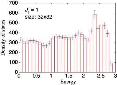
Figure 10: Density of states of quasi-particles at $J_{1}=J_{2}=J_{3}=1$ in gapless phase. The quasi-particle energies $\epsilon_{\mu}$ are computed for systems with $32\times 32$ unit cells and the histogram of them is obtained. The bin is set at $0.1$. The average is takes over $10000$ instances of $\{D_{\vec{n}}\}$. The density of states with small energy takes a finite value and fluctuates. The amplitude of fluctuation is comparable with the error bars. This result suggests $D(\varepsilon)$ is a constant when $\varepsilon$ is small.

The scaling laws in Eq. (40) can be also obtained by another argument. To elucidate this, we show, in Fig. 11, the low-lying energy spectra of quasi-particles of the model as a function of $J_{3}$ for finite sized system ($8\times 8$ unit cells) for a single configuration of $\{D_{\vec{n}}\}$. Since there is a finite gap for all values of $J_{3}$, an adiabatic evolution do not lead to quasi-particle excitation. For non-adiabatic processes, the most probable excitation occurs around the avoided level crossing with minimum energy gap shown with a blue arrow in Fig. 11. We denote the corresponding energy gap by $\Delta_{l}$. The probability of excitation is well approximated by the Landau-Zener formula: $e^{-c\Delta_{l}^{2}\tau}$, where $c$ is a constant factor determined by the slope of the excitation gap around $\Delta_{l}$. Next, we recall that the distribution of excitation gaps $\Delta$ for fixed $J_{3}$ inside the gapless phase scales as $1/L^{2}$. Hence the distribution of $\Delta_{l}$ is also a function of $\Delta_{l}L^{2}$. Thus the probability distribution function of $\Delta_{l}$ can be written as $P(u)$ with $u=\Delta_{l}L^{2}$. Assuming that the factor $c$ is independent of $L$ and $\Delta_{l}$, the averaged probability of excitation $n$ is given by

$$n \sim \int_{0}^{\infty}duP(u)e^{-c\Delta_{l}^{2}\tau}=\int_{0}^{\infty}duP(u)e^{-cu^{2}\tau/L^{4}}$$ (41)

$$= \Pi(\tau/L^{4}).$$

From this, one can obtain a length $L_{\varepsilon}$ that yields averaged probability of excitation $\Pi=\varepsilon$ for a given $\tau$: $L_{\varepsilon}=\left(\frac{\tau}{\Pi^{-1}(\varepsilon)}\right)^{1/4}$. For sufficiently small $\varepsilon$, $N_{\varepsilon}=L_{\varepsilon}^{2}$ is regarded as the average size within which a single excitation is expected to occur. The density of these excitations is thus estimated by $N_{\varepsilon}$ as

$$n\sim\frac{1}{N_{\varepsilon}}=\left(\frac{\Pi^{-1}(\varepsilon)}{\tau}\right)^{1/2}\propto\tau^{-1/2}.$$ (42)

Figure 11: Low-lying positive eigenvalues of $M$ as a function of $J_{3}$ with a fixed configuration of $\{D_{\vec{n}}\}$. The system is composed of $8\times 8$ unit cells.

Note that these arguments do not depend on whether the quench ends inside the gapless phase or not since for slow dynamics the defects are produced mostly during the passage through the gapless regime. Using the fact that $p=0$ for these systems, a similar analysis for $Q$ reproduces the results of Eq. (40).

V Discussion

In conclusion, we have shown that the Kitaev model constitutes an example of a two-dimensional model with an anisotropic critical point. We have also demonstrated that the presence of such an anisotropic critical point leads to novel scaling laws defect density and residual energy during slow power-law dynamics which takes the system from a gapped phase to the vicinity of such a critical point. We have generalized our results for such scaling laws for $d$-dimensional systems with such anisotropic critical point. Further, we have computed all independent correlation functions of the Kitaev model in the Fermionic representation after a slow linear ramp which brings the system to the vicinity of an anisotropic critical point. We have charted out the spatial dependence of the correlation function and discussed its relation with several multiple spin correlators of the model. Finally, we have studied the non-equilibrium slow dynamics of the disordered Kitaev model where disorder is introduced via random configuration of $D_{\vec{n}}$ in its Fermionic representation. We have shown numerically that the defect density $n$, generated during a slow linear ramp from a gapped phase of the model to either a gapless phase or to another gapped phase through a gapless region, scales as $\tau^{-1/2}$. In contrast, the residual energy $Q$ scales as $\tau^{-1/2}$ ($\tau^{-1}$) for similar dynamics ending on the gapless surface (gapped phase after passing through the gapless surface). We provide a qualitative understanding of such scaling laws to back up our numerical results. We note that there has been suggestions of experimental realization of the Kitaev model using ultracold atomic system blochrev . In the event of such a realization, the simplest experimental test of our theory would involve measurement of defect density $n$ following a slow ramp. Such experiments has recently been performed for standard ultracold boson systems greiner1 .

The authors thank A. Dutta, K. Kubo, A. Polkovnikov, G. Santoro and D. Sen for discussions. KS thanks DST, India for support through grant SR/S2/CMP-001/2009. SS acknowledges support from Grant-in-Aid for Scientific Research from MEXT, Japan.