First-Passage Exponents of Multiple Random Walks

Abstract

We investigate first-passage statistics of an ensemble of $N$ noninteracting random walks on a line. Starting from a configuration in which all particles are located in the positive half-line, we study $S_{n}(t)$, the probability that the $n$th rightmost particle remains in the positive half-line up to time $t$. This quantity decays algebraically, $S_{n}(t)\sim t^{-\beta_{n}}$, in the long-time limit. Interestingly, there is a family of nontrivial first-passage exponents, $\beta_{1}<\beta_{2}<\cdots<\beta_{N-1}$; the only exception is the two-particle case where $\beta_{1}=1/3$. In the $N\to\infty$ limit, however, the exponents attain a scaling form, $\beta_{n}(N)\to\beta(z)$ with $z=(n-N/2)/\sqrt{N}$. We also demonstrate that the smallest exponent decays exponentially with $N$. We deduce these results from first-passage kinetics of a random walk in an $N$-dimensional cone and confirm them using numerical simulations. Additionally, we investigate the family of exponents that characterizes leadership statistics of multiple random walks and find that in this case, the cone provides an excellent approximation.

I Introduction

Ensembles of ordinary random walks in one dimension wf ; ghw ; hcb ; rg are used to model physical, chemical, and biological processes ranging from wetting mef ; hf to the motion of colloidal particles in narrow channels wbl ; cdl and reaction-diffusion processes bpl . In particular, first-passage properties sr of multiple random walks explain dynamics of interacting spins dhp ; snm , lead changes in a voting process wf ; hn , and lifetime of knots in polymer chains bdve .

In these examples, first-passage properties are intertwined with the ordering of the walkers mef ; hf ; fg ; bg ; djg ; kr ; bjmkr ; ck ; dlb ; yal . Previous studies focused on first-passage statistics of extreme particles; for example, the probability that a single prey particle survives the predators to its left bg ; kr . These problems involve a single first-passage probability and hence, a single first-passage exponent sr .

In this paper, we ask first-passage questions that concern the bulk particles, not necessarily the extreme ones. We find that a family of first-passage exponents characterizes the first-passage kinetics. These exponents depend on two parameters: the particle order and the total number of particles. Yet, when the number of particles is very large, the exponents depend on a single scaling variable. This scaling behavior is unusual. In equilibrium as well as in non-equilibrium settings, one or two scaling exponents quantify a scaling behavior gib ; hes . In the present case, however, the exponents themselves obey scaling, and remarkably, there are scaling laws for the scaling exponents.

Figure 1: Illustration of a four-particle system. Initially, all particles are located in the positive half-line. At time $t$, the position of the rightmost particle is $x_{1}(t)$ and that of the leftmost particle is $x_{4}(t)$.

We consider an array of $N$ identical particles that undergo simple random walk on a one-dimensional line, and investigate two different first-passage problems where the particle order plays an essential role. The first problem, discussed in Sections II-V, concerns the probability that the $n$th rightmost particle hasn’t crossed the origin, if all particles start to the right of the origin (Figure 1). This quantity equals the likelihood that $N-n+1$ out of all random walks have yet to simultaneously reside in the negative half-line. In the second problem, described in Section VI, we identify the particle order with rank, such that the rightmost particle is viewed as the leader, and similarly, the leftmost particle as the laggard. We ask: what is the probability that the rank of the initial leader does not fall below some specified threshold?

In both problems, we find a family of nontrivial first-passage exponents. In both cases, the exponents depend on two variables: the particle order and the total number of particles, $N$. Interestingly, in the large-$N$ limit, the exponents become a function of a single scaling variable. However, the similarities between the two problems end here as the two scaling variables are fundamentally different and moreover, the two scaling functions are dissimilar.

Our analysis relies on mapping the $N$ noninteracting random walks onto a single compound random walk in $N$ dimensions. By combining this mapping with exact and asymptotic properties for kinetics of first-passage inside a cone bk , we obtain approximate values for the first-passage exponents. The cone approximation is straightforward to implement, yet it yields useful estimates for exponents and in particular, this framework faithfully captures typical and extremal properties of the first-passage exponents.

II The First-Passage Process

Our system consists of $N$ identical particles. Each particle undergoes a random walk on a one-dimensional lattice. At every time step, one particle is selected at random, and it moves to the left, $x\to x-1$, or to the right $x\to x+1$, with equal probabilities. Time is augmented by the inverse number of particles after each such step, $t\to t+1/N$. The particles always undergo independent random walks and hence, they are noninteracting.

Let $x_{n}(t)$ be the position of the $n$th rightmost particle at time $t$ (Figure 1). We consider the initial configuration where all particles are located in the positive half-line (Figure 1), $x_{n}(0)>0$ for all $n$. We stress that it is not the initial order, but instead, the order at time $t$, that sets the index $n$.

We are interested in $S_{n}(t)$, the probability that the $n$th rightmost particle remains in the positive half-line until time $t$. Hence, $S_{n}(t)$ is the likelihood that $x_{n}(\tau)>0$ for all $0\leq\tau\leq t$. In particular, $S_{1}(t)$ is the probability that the rightmost particle has yet to cross the origin, while $S_{N}(t)$ is the probability that the leftmost particle has not crossed the origin. Clearly, the probabilities $S_{n}$ decrease monotonically with $n$,

$$S_{1}(t)\geq S_{2}(t)\geq\cdots\geq S_{N-1}(t)\geq S_{N}(t).$$ (1)

The “survival” probabilities $S_{n}(t)$ generalize the classic survival probability of a single one-dimensional random walk in the presence of a trap. Indeed, when $N=1$, we have $S_{1}(t)\sim t^{-1/2}$ sr . As usual, the survival probability $S_{n}$ immediately gives the first-passage probability as $[-dS_{n}/dt]\times dt$ is the probability that the $n$th rightmost particle crosses the origin for the first time during the infinitesimal time interval $(t,t+dt)$.

The analytically solvable case of two particles yields valuable insights into the general behavior. When $N=2$, we map the two random walks onto a single random walk in two dimensions. The position of the two-dimensional walk is specified by the positions of the two independent walks. At $t=0$, the two-dimensional walk is always inside the first quadrant (Figure 2).

Figure 2: The compound two-dimensional random walk. The line indicates the random walk trajectory and the bullets show intermediate locations along this trajectory. Thick lines mark the absorbing boundary. (a) For $n=1$, the random walk is confined to the exterior of the third (negative) quadrant. (b) For $n=2$, the random walk is confined to the interior of the first (positive) quadrant.

The quantity $S_{1}(t)$ is the probability that the coordinates of the two random walks have not become negative simultaneously up to time $t$, or equivalently, the probability that the two-dimensional walk remains in the exterior of the third quadrant (Figure 2a). To find the survival probability, we impose an absorbing boundary condition along the edge of the third quadrant (Figure 2a). Then $S_{1}(t)$ is the probability that the compound particle avoids this absorbing boundary up to time $t$. The region in which the random walk can move is a two-dimensional cone, or equivalently, a wedge with opening angle $\alpha=3\pi/4$. (The opening angle $\alpha$ is defined as the angle between the cone axis and the cone surface, so it lies within the bounds $0\leq\alpha\leq\pi$.) Thus, $S_{1}(t)$ equals the survival probability of a particle diffusing inside a wedge with an absorbing surface. This survival probability decays algebraically,

$$S(t)\sim t^{-\pi/4\alpha},$$ (2)

in the long-time limit sr . By substituting $\alpha=3\pi/4$ into the general expression (2), we find the intriguing behavior

$$S_{1}(t)\sim t^{-1/3},$$ (3)

as $t\to\infty$. As in (2), this asymptotic behavior holds regardless of the initial position, although the prefactor does depend on the initial conditions.

Along the same lines, $S_{2}(t)$ is the probability that the positions of the two random walks remain positive up to time $t$, or alternatively, the probability that the two-dimensional walk remains in the interior of the first quadrant (Figure 2b). Now, the boundary of the first quadrant is absorbing (Figure 2b), and the random walk is confined to a wedge with opening angle $\alpha=\pi/4$. Using (2), we again find power-law behavior albeit with a larger exponent,

$$S_{2}(t)\sim t^{-1}.$$ (4)

As shown below, this particular behavior follows from an elementary argument.

III A Family of Exponents

The analytic results for a two-particle system suggest that generally, the survival probabilities decay algebraically,

$$S_{n}(t)\sim t^{-\beta_{n}},$$ (5)

in the long-time limit. Moreover, we expect that the decay exponents are distinct, and that $\beta_{n}\equiv\beta_{n}(N)$ increases monotonically with $n$,

$$\beta_{1}<\beta_{2}<\cdots<\beta_{N-1}<\beta_{N},$$ (6)

consistent with (1).

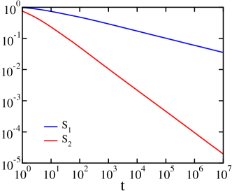
Figure 3: The survival probabilities $S_{1}(t)$ and $S_{2}(t)$ for three particles. These results are from numerical simulations.

N	$\beta_{1}$	$\beta_{2}$	$\beta_{3}$	$\beta_{4}$	$\beta_{5}$	$\beta_{6}$
$1$	1/2
$2$	1/3	1
$3$	$0.228$	$0.68$	3/2
$4$	$0.158$	$0.50$	$1.05$	2
$5$	$0.107$	$0.358$	$0.76$	$1.37$	5/2
$6$	$0.071$	$0.261$	$0.584$	$1.05$	$1.7$	3

Table 1: The exponent $\beta_{n}$, obtained from numerical simulations for $N\leq 6$.

The largest exponent, $\beta_{N}$, is trivial. The probability $S_{N}(t)$ that the leftmost particle has yet to cross the origin equals the probability that not a single particle crossed the origin. Since the particles are independent, this probability equals the product of the individual probabilities for each particle not to cross the origin, $S_{N}\sim\left(t^{-1/2}\right)^{N}\sim t^{-N/2}$. Therefore, the largest exponent is proportional to the total number of particles,

$$\beta_{N}=\tfrac{1}{2}N\,.$$ (7)

Our numerical simulations confirm that indeed, there are $N$ distinct first-passage exponents. Figure 3 shows the survival probabilities $S_{1}$ and $S_{2}$ for a three-particle system, and Table I lists the exponents $\beta_{n}$ for $N\leq 6$. The simulations confirm that there is a family of $N-1$ nontrivial exponents, $\{\beta_{1},\beta_{2},\ldots,\beta_{N-1}\}$.

We performed extensive Monte Carlo simulations using the following algorithm. Initially, all $N$ particles are located at the same position, $x=1$. In each subsequent step one particle is selected at random and it moves by one lattice site either to the left or to the right with equal probabilities. After each step, time is augmented by the inverse number of particles, $t\to t+1/N$. Throughout this random process, we keep track of the total number of particles in the region $x<0$, and obtain the probability $S_{n}(t)$ from the fraction of realizations in which this counter did not exceed $n$ until time $t$. We computed the exponents $\beta_{n}$ by analyzing the local slope $-d\ln S_{n}/d\ln t$ or alternatively, by seeking the value of $\beta_{n}$ for which the quantity $t^{\beta_{n}}S_{n}(t)$ achieves a plateau (Figure 4).

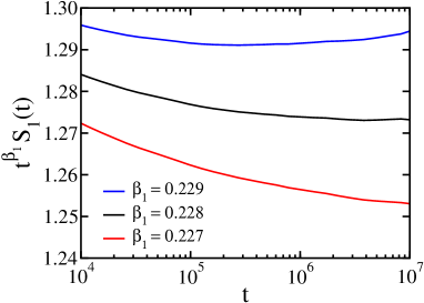
Figure 4: The function $t^{\beta_{1}}\,S_{1}(t)$ versus $t$, using different values of $\beta_{1}$. The data is from numerical simulations of a three-particle system.

We verified that the measured exponents $\beta_{n}$ are robust. First, we checked that they are not sensitive to the initial positions. Second, we used parallel dynamics where particles move synchronously, rather than sequentially, and found that the exponents do not change. The exponents reported in this study represent an average over a large number of independent realizations. The total number of realizations varies from $10^{6}$ for slow first-passage processes ($\beta\ll 1$) to as high as $10^{12}$ for fast processes ($\beta\gg 1$). We note that it is difficult to measure tiny exponents $\beta\ll 1$ because the simulations must run to very large times, and furthermore, it is difficult to obtain large exponents $\beta\gg 1$, because now, we need an enormous number of realizations.

As a side note, the behavior (5)-(6) has a natural interpretation in the context of single-file diffusion where the random walks interact by hard core exclusion teh ; dgl ; ap ; vkk ; tw ; ra ; krb . Under the standard transformation where the identities of two particles are exchanged whenever their trajectories cross, the noninteracting particle system is equivalent to an interacting particle system. In the context of this exclusion process, the quantity $S_{n}(t)$ is the probability that the $n$th out of $N$ particles avoids the negative half-line up to time $t$.

IV Cone Approximation

In general, we map the $N$ one-dimensional random walks onto a single random walk in $N$ dimensions. To find the survival probability $S_{n}(t)$, we require that the random walk remains inside the region in which the number of negative coordinates is smaller than $n$ up to the $t$. This region occupies a fraction $V_{n}$ of space given by

$$V_{n}=2^{-N}\sum_{m=n}^{N}\binom{N}{m}.$$ (8)

For example, when $N=2$ we have $(V_{1},V_{2})=(3/4,1/4)$ as in Fig. 2, while $(V_{1},V_{2},V_{3})=(7/8,1/2,1/8)$ for $N=3$.

In two dimensions, the random walk is confined to two-dimensional cones of opening angles $\alpha=3\pi/4$ and $\alpha=\pi/4$ when $n=1$ and $n=2$, respectively. In the cone approximation, we replace the region of space that confines the walk with an unbounded circular cone in $N$ dimensions that occupies the same fraction of space $V_{n}$. An $N$-dimensional cone with opening angle $\alpha$ occupies the fraction of space

$$V(\alpha)=\frac{\int_{0}^{\alpha}d\theta\,(\sin\theta)^{N-2}}{\int_{0}^{\pi}d\theta\,(\sin\theta)^{N-2}}.$$ (9)

Using a spherical coordinate system, this expression follows from $d\Omega\propto(\sin\theta)^{N-2}d\theta$ where $\Omega$ is the solid angle and $\theta$ is the polar angle. We now choose the cone opening angle $\alpha\equiv\alpha(n,N)$ as follows

$$V(\alpha)=V_{n}.$$ (10)

N	$\beta_{1}^{\rm cone}$	$\beta_{2}^{\rm cone}$	$\beta_{3}^{\rm cone}$	$\beta_{4}^{\rm cone}$	$\beta_{5}^{\rm cone}$	$\beta_{6}^{\rm cone}$
$2$	1/3	1
$3$	$0.216785$	$1/2$	$1.407279$
$4$	$0.139844$	$0.337987$	$0.739671$	$1.787705$
$5$	$0.0893854$	$0.237106$	$1/2$	$0.998423$	$2.151625$
$6$	$0.0564058$	$0.166833$	$0.359218$	$0.684043$	$1.265701$	$2.503786$

Table 2: The exponents $\beta_{n}^{\rm cone}$, obtained using the cone approximation, that is, Eqs. (8)–(11).

The survival probability of a particle that diffuses inside an unbounded $N$-dimensional cone decays algebraically, $S\sim t^{-\beta}$, in the long-time limit sr ; rdd ; bs . The exponent $\beta\equiv\beta(\alpha)$ decreases as the opening angle $\alpha$ increases. In two dimensions, $\beta=\pi/4\alpha$ as in (2), and in four dimensions $\beta=(\pi-\alpha)/2\alpha$ bk . Generally, the decay exponent $\beta$ is the smallest root of a transcendental equation involving either $P_{2\beta+\delta}^{\delta}$ or $Q_{2\beta+\delta}^{\delta}$, that is, one of the two associated Legendre functions NIST of degree $2\beta+\delta$ and order $\delta=\frac{N-3}{2}$ bk ,

$$\begin{split}P_{2\beta+\delta}^{\delta}(\cos\alpha)&=0\qquad N\ {\rm odd},\\ Q_{2\beta+\delta}^{\delta}(\cos\alpha)&=0\qquad N\ {\rm even}.\end{split}$$ (11)

In three dimensions, the transcendental equation involves the Legendre function, $P_{2\beta}(\cos\alpha)=0$. In all dimensions, a cone with $\alpha=\pi/2$ is simply a plane, and hence $\beta(\pi/2)=1/2$.

By construction, the cone approximation is exact in two dimensions. For three particles, the cone approximation provides good estimates for the smallest and the largest exponents. When $n=1$, the cone specified by (10) has opening angle $\alpha_{1}=\pi-0.722734$ , and equation (11) gives the first-passage exponent $\beta_{1}^{\rm cone}=0.216785$ where the superscript indicates outcome of the cone approximation. This value represents a very good approximation, as the simulations yield $\beta_{1}=0.228$. For the largest exponent ($n=3$) the opening angle is $\alpha_{3}=0.722734$ and the consequent value $\beta_{3}^{\rm cone}=1.407279$ is close to the exact value $\beta_{3}=3/2$. When $n=2$, there is a larger discrepancy: $\alpha_{2}=\pi/2$ leads to the approximate value $\beta_{2}^{\rm cone}=1/2$, while the simulations yield $\beta_{2}=0.68$.

Table II lists the outcome of the cone approximation for $2\leq N\leq 6$. Comparing with the respective values in Tables I, we see that quantitatively, the cone approximation deteriorates as $N$ grows. Nevertheless, the cone approximation faithfully captures all qualitative features of the first-passage exponents, as shown below.

V Scaling and Extremal Properties

We are especially interested in the behavior when the number of particles is large, $N\gg 1$. Let us first evaluate the fraction $V_{n}$ in the limit $N\to\infty$. Using the Stirling formula $N!\simeq\sqrt{2\pi N}\,N^{N}\,e^{-N}$ we write the leading behavior of the binomial term in (8),

$$2^{-N}\binom{N}{m}\simeq\sqrt{2/\pi N}\,e^{-2(m-N/2)^{2}/N}.$$

We now take the continuum limit and convert the sum on the right hand side of (8) into an integral. The quantity $V_{n}$ becomes a function of a single scaling variable

$$V_{n}(N)\to\frac{1}{2}\,{\rm erfc}\left(z\sqrt{2}\right)\quad{\rm with}\quad z=\frac{n-N/2}{\sqrt{N}},$$ (12)

where ${\rm erfc}(\xi)=(2/\sqrt{\pi})\int_{\xi}^{\infty}e^{-u^{2}}du$ is the complementary error function. Equation (12) is valid in the limit $n,N\to\infty$ with the scaling variable $(n-N/2)/\sqrt{N}$ finite.

Similarly, we evaluate the leading large-$N$ behavior of $V(\alpha)$ given in (9). The dominant contribution to the integral comes from a narrow region of order $1/\sqrt{N}$ in the vicinity of $\alpha=\pi/2$ where the integrand is Gaussian,

$$(\sin\theta)^{N-2}\simeq e^{-N(\pi/2-\theta)^{2}/2}.$$

Using the leading asymptotic behavior of the denominator, $\int_{-\infty}^{\infty}\exp\big{[}\!-\!N(\pi/2-\theta)^{2}/2\big{]}d\theta\to\sqrt{2\pi/N}$, we find that the fraction $V(\alpha)$ has the scaling form

$$V(\alpha,N)\to\frac{1}{2}\,{\rm erfc}\left(\frac{y}{\sqrt{2}}\right)\quad{\rm with}\quad y=(\cos\alpha)\sqrt{N}.$$ (13)

In writing this equation, we used the fact $\cos\alpha\simeq\pi/2-\alpha$ when $\pi/2-\alpha\to 0$. Equation (13) is valid in the limit $\pi/2-\alpha\to 0$, $N\to\infty$, with the scaling variable $(\cos\alpha)\sqrt{N}$ finite. Meanwhile, asymptotic analysis of (11) shows that in the limit $N\to\infty$, $\pi/2-\alpha\to 0$ with the scaling variable $(\cos\alpha)\sqrt{N}$ finite, the exponent $\beta(\alpha)$ becomes a function of the scaling variable $y$ alone,

$$\beta(\alpha,N)\to\beta(y)\quad{\rm with}\quad y=(\cos\alpha)\sqrt{N}.$$ (14)

The dependence of the exponent $\beta$ on the scaling variable $y$ is specified through the transcendental equation $D_{2\beta}(y)=0$, where $D_{\nu}$ is the parabolic cylinder function NIST of order $\nu$, and the acceptable root is the smallest one bk .

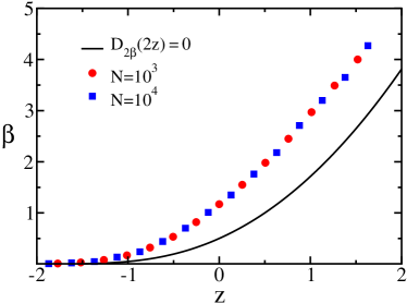
Figure 5: The exponent $\beta$ versus the scaling variable $z$. The Monte Carlo results are from simulations with $N=10^{3}$ (bullets) or $N=10^{4}$ (squares) particles. The solid line is the scaling function (16) obtained using the cone approximation.

Comparing equation (12) with equation (13), we conclude that the first-passage exponent depends on a single scaling variable,

$$\beta_{n}(N)\to\beta(z)\quad{\rm with}\quad z=\frac{n-N/2}{\sqrt{N}},$$ (15)

in the large-$N$ limit. Using $y=2z$, the exponent $\beta$ and the scaling variable $z$ are related by the transcendental equation

$$D_{2\beta}(2z)=0.$$ (16)

In particular, $\beta(z=0)=1/2$ (Figure 5).

The scaling behavior (15)–(16) implies that the exponents $\beta_{n}$ are of order one only in a window of size $\sqrt{N}$ centered on the mid-point $n=N/2$. Otherwise, the exponents are exponentially small when $N/2-n\gg\sqrt{N}$, or algebraically large when $n-N/2\gg\sqrt{N}$. The limiting behaviors of the scaling function captures these extremal properties,

$$\beta^{\rm cone}(z)\simeq\begin{cases}\sqrt{z^{2}/2\pi}\,\exp\!\left(-2z^{2}\right)&z\to-\infty\\ z^{2}/2&z\to\infty.\end{cases}$$ (17)

Both of these limiting behaviors follow from (16), see bk . The algebraic behavior in the limit $z\to\infty$ implies $\beta_{N}\sim N$, in agreement with (7).

Results of massive numerical simulations with a large number of particles confirm (Fig. 5) that the first-passage exponents adhere to the scaling form (15). Moreover, the shape of the scaling function is qualitatively similar to the shape of the scaling function (16).

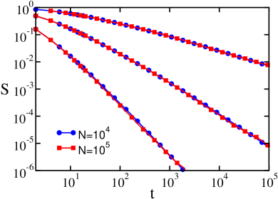
Figure 6: The survival probability $S(z,t)$ versus time $t$. Shown are results of simulations with different number of particles, $N=10^{4}$ (bullets) and $N=10^{5}$ (squares), at three different values of the scaling variable, $z=-1/2$ (upper curves), $z=0$ (intermediate curves), and $z=1/2$ (lower curves).

Additionally, the simulations reveal (Fig. 6) that not only the scaling exponents depend on a single scaling variable, but the entire survival probability is also function of the scaling variable $z$. That is,

$$S_{n}(t)\to S(z,t)\quad{\rm with}\quad z=\frac{n-N/2}{\sqrt{N}}$$ (18)

when $N\gg 1$. We confirmed this behavior numerically using a very large number of particles (Figure 6). The scaling behavior (18) is notable because it applies at all times: it holds at short times, at intermediate times, and at long times.

Of special interest is the survival probability of the median particle which becomes completely independent of the total number of particles when $N\to\infty$. There is an interesting limiting value that characterizes the survival probability of the median particle,

$$\beta_{\rm mid}=\lim_{N\to\infty}\beta_{N/2}.$$ (19)

Numerically, $\beta_{\rm mid}=1.16$, while the cone approximation gives $\beta_{\rm mid}=1/2$. This universal behavior and the scaling form (15) show that there is a narrow “scaling-window” of width $\Delta n$ with $\Delta n/N\sim N^{-1/2}$ centered on the median particle. Hence, only the relatively small number of particles residing inside this region influence the median particle. This behavior is in line the narrow range of cone opening angles, $\Delta\alpha\sim N^{-1/2}$, where the first-passage exponents change rapidly according to (14).

The smallest exponent $\beta_{1}$ underlying the decay of $S_{1}(t)$ is especially intriguing because $S_{1}(t)$ has a simple interpretation — it is the probability that the $N$-dimensional walk remains in the exterior of the generalized $N$-dimensional “quadrant” (see Figure 2), a region that occupies a fraction $V_{1}=1-2^{-N}$ of space. Table III shows that the cone approximation yields useful estimates for $\beta_{1}$ when $N$ is small. The cone approximation is also useful for understanding the large-$N$ behavior. Substituting $V_{1}=1-2^{-N}$ into (10) and $[\sin(\pi-\theta)]^{N}\simeq(\pi-\theta)^{N}$ into (9), we readily find that the opening angle approaches a constant,

$$\alpha\to\pi-\frac{1}{2},$$ (20)

in the limit $N\to\infty$. In a cone of fixed opening angle $\alpha>\pi/2$, the survival exponent $\beta$ shrinks exponentially with dimension, $\beta\sim[\sin(\pi-\alpha)]^{N}$ in the large-$N$ limit bk . Thus, we conclude that the smallest exponent decays exponentially with the total number of particles,

$$\beta_{1}\sim e^{-C\,N},$$ (21)

with $C^{\rm cone}=-\ln(\sin\tfrac{1}{2})=0.735167$. The simulation results are consistent with this exponential decay (Fig. 7).

N	$\beta_{1}^{\rm cone}$	$\beta_{1}$
$2$	$1/2$	$1/2$
$3$	$0.216785$	$0.228$
$4$	$0.139844$	$0.156$
$5$	$0.0893854$	$0.106$
$6$	$0.0564058$	$0.0710$
$7$	$0.0350414$	$0.0467$
$8$	$0.0213967$	$0.0310$
$9$	$0.01283556$	$0.0189$
$10$	$0.00756816$	$0.0123$

Table 3: The smallest exponent as a function of $N$. Listed are the outcome of the cone approximation, $\beta_{1}^{\rm cone}$, and the results of numerical simulations, $\beta_{1}$.

The exponential decay (21) and the algebraic growth (6) imply the following limiting behaviors of $\beta$ in the scaling regime,

$$\beta(z)\sim\begin{cases}\exp\left(-{\rm const.}\times z^{2}\right)&z\to-\infty,\\ z^{2}&z\to\infty.\end{cases}$$ (22)

These behaviors are fully consistent with (17). Therefore, the cone approximation captures all qualitative features of the first-passage exponents including typical behavior that includes the form of the scaling variable and the shape of the scaling function, as well as extremal behavior comprising of exponential decay of the smallest exponent and algebraic growth of the largest exponent largest .

VI Leadership Statistics

The cone approximation is useful in other contexts. We now apply this approach to understand leadership statistics of multiple random walks.

We study the very same system of $N$ independent random walks in one dimension. As shown in Figure 1, we rank the particles by position with $n=1$ being the rightmost particle and $n=N$ being the leftmost particle. As if the random walks participate in a competition kr ; bjmkr ; bh ; bmr ; abk , we view the rightmost particle as leader and the leftmost particle as laggard. We now investigate $P_{n}(t)$, the probability that the rank of the particle initially in the lead, does not fall below $n$ up to time $t$. Thus, $P_{1}(t)$ is the probability that the original leader never loses the lead, while $P_{N-1}(t)$ is the probability that the original leader does not become the laggard.

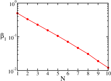
Figure 7: The smallest exponent, $\beta_{1}$, versus the total number of particle $N$. The results are from Monte Carlo simulations.

If $N=2$, we have $P_{1}\sim t^{-1/2}$. For three particles, $P_{1}(t)\sim t^{-3/4}$ and $P_{2}\sim t^{-3/8}$ bjmkr . In this case, the compound random walk in two dimensions is confined to wedges formed by two intersecting planes. These wedges occupy fractions $V_{1}=1/3$ and $V_{2}=2/3$ of space, and the decay exponents are given by $\gamma=\pi/4\alpha$ or equivalently, $\gamma=1/4V$. Based on the results for two- and three-particle systems, we expect that the probabilities $P_{n}$ decay algebraically,

$$P_{n}(t)\sim t^{-\gamma_{n}},$$ (23)

in the long-time limit. Once again, there is a family of first-passage exponents,

$$\gamma_{1}>\gamma_{2}>\cdots>\gamma_{N-1}.$$ (24)

The largest exponent $\gamma_{1}$ characterize the probability that the initial leader maintains the lead, and the smallest exponent $\gamma_{N-1}$ characterizes the probability that the original leader never turns into the laggard.

In this case, the compound $N$-dimensional walk moves in a region that occupies a fraction

$$V_{n}=\frac{n}{N}$$ (25)

of space. For example, to see that $V_{1}=1/N$ we note that the total $N$-dimensional space is divided into $N$ equivalent regions in which the identity of the leader is the same. It is straightforward to generalize this result to all $n$. We have seen that when there are three particles, the boundary of the allowed region forms a two-dimensional cone. We therefore replace the allowed region with an $N-1$ dimensional cone occupying the same fraction of space (25) as the allowed region. The opening angle of this cone, $\alpha$, satisfies

$$\frac{\int_{0}^{\alpha}d\theta\,(\sin\theta)^{N-3}}{\int_{0}^{\pi}d\theta\,(\sin\theta)^{N-3}}=\frac{n}{N}.$$ (26)

Given $n$ and $N$, we first determine the opening angle $\alpha$ by solving (26), and then compute the exponent $\gamma$ as the smallest root of a transcendental equation involving one of the two associated Legendre functions with degree $2\gamma+\mu$ and order $\mu=\frac{N-4}{2}$,

$$\begin{split}P_{2\gamma+\mu}^{\mu}(\cos\alpha)&=0\qquad N\ {\rm even},\\ Q_{2\gamma+\mu}^{\mu}(\cos\alpha)&=0\qquad N\ {\rm odd}.\end{split}$$ (27)

By construction, the cone approximation is exact for three particles. The cone approximation values, listed in Table IV, provide very good estimates, given the Monte Carlo simulation values listed in Table V. The numerical simulations are implemented using the algorithm described in Section III, except that at time $t=0$, the random walks occupy $N$ consecutive lattice sites.

N	$\gamma_{1}^{\rm cone}$	$\gamma_{2}^{\rm cone}$	$\gamma_{3}^{\rm cone}$	$\gamma_{4}^{\rm cone}$	$\gamma_{5}^{\rm cone}$
$3$	$3/4$	$3/8$
$4$	$0.888644$	$1/2$	$0.300754$
$5$	$0.986694$	$0.612148$	$0.408397$	$0.253371$
$6$	$1.062297$	$0.701508$	$1/2$	$0.351915$	$0.220490$

Table 4: The exponents $\gamma_{n}^{\rm cone}$, obtained using a cone in $N-1$ dimensions with fraction of space $V_{n}=n/N$.

N	$\gamma_{1}$	$\gamma_{2}$	$\gamma_{3}$	$\gamma_{4}$	$\gamma_{5}$
$2$	1/2
$3$	$3/4$	$3/8$
$4$	$0.913$	$0.556$	$0.306$
$5$	$1.02$	$0.676$	$0.454$	$0.265$
$6$	$1.11$	$0.769$	$0.557$	$0.391$	$0.234$

Table 5: The exponent $\gamma_{n}$ from numerical simulations.

From (26), we expect that the exponent $\gamma$ depends on a single scaling variable,

$$\gamma_{n}(N)\to\gamma(x)\quad{\rm with}\quad x=\frac{n}{N},$$ (28)

in the limit $N\to\infty$. When $N$ is very large, we can replace the left-hand side in (26) with the right-hand side in (9). Substituting (25) into (13) shows that

$$y=\sqrt{2}\,{\rm erfc}^{-1}(2x).$$ (29)

Here ${\rm erfc}^{-1}(x)$ is the inverse complementary error function, (see below equation (12)). Using the scaling behavior (16), we find that $\gamma$ and $x$ are related by the transcendental equation (Figure 8)

$$D_{2\gamma}\left(\sqrt{2}\,{\rm erfc}^{-1}(2x)\right)=0,$$ (30)

where $D_{\nu}$ is the parabolic cylinder function. We note that $\gamma(0)=1/2$. Given the definition of $x$, the scaling behavior in the leadership problem is completely different than the scaling behavior in the origin-crossing problem.

N	$\gamma_{N-1}^{\rm cone}$	$\gamma_{N-1}$
$2$	$1/2$	$1/2$
$3$	$3/8$	$3/8$
$4$	$0.300754$	$0.306$
$5$	$0.253371$	$0.265$
$6$	$0.220490$	$0.234$
$7$	$0.196216$	$0.212$
$8$	$0.177469$	$0.190$
$9$	$0.162496$	$0.178$
$10$	$0.150221$	$0.165$

Table 6: The smallest exponent as a function of $N$. Listed are estimates from the cone approximation, $\gamma_{N-1}^{\rm cone}$, and results of numerical simulations, $\gamma_{N-1}$.

N	$\gamma_{1}^{\rm cone}$	$\gamma_{1}$
$3$	$3/4$	$3/4$
$4$	$0.888644$	$0.91$
$5$	$0.986694$	$1.02$
$6$	$1.062297$	$1.11$
$7$	$1.123652$	$1.19$
$8$	$1.175189$	$1.27$
$9$	$1.219569$	$1.33$
$10$	$1.258510$	$1.37$

Table 7: The largest exponent as a function of $N$. Listed are the estimates from the cone approximation, $\gamma_{1}^{\rm cone}$, and results of numerical simulations, $\gamma_{1}$.

Using the asymptotic behaviors

$${\rm erfc}(\xi)\simeq\begin{cases}2-\big{(}\sqrt{1/\pi\xi^{2}}\,\big{)}\exp(-\xi^{2})&\xi\to-\infty,\\ \big{(}\sqrt{1/\pi\xi^{2}}\,\big{)}\,\exp(-\xi^{2})&\xi\to\infty,\end{cases}$$

we deduce that the variable $y$ defined in (29) has the asymptotic behaviors

$$y(x)\simeq\begin{cases}\sqrt{2\ln\frac{1}{2x}}&x\to 0,\\ -\sqrt{2\ln\frac{1}{2(1-x)}}&x\to 1.\end{cases}$$

Substituting these expressions into the asymptotic behavior of the scaling function in (14), we find the limiting behaviors (see also bk )

$$\gamma(x)\simeq\begin{cases}\frac{1}{4}\ln\frac{1}{2x}&x\to 0,\\ (1-x)\ln\frac{1}{2(1-x)}&x\to 1.\end{cases}$$ (31)

The exponent $\gamma$ decreases monotonically with $x$: it weakly diverges when $x\to 0$ and it vanishes as $x\to 1$. By substituting $x=1/N$ and $1-x=1/N$, respectively, into the appropriate expressions in (31), we find the leading large-$N$ behaviors

$$\gamma_{n}\simeq\begin{cases}\frac{1}{4}\ln N&n=1,\\ \frac{1}{N}\ln N&n={N-1}.\end{cases}$$ (32)

Both expressions match estimates based on heuristic arguments kr ; bjmkr . The smallest and the largest exponents, listed respectively in Tables VI-VII, show that the cone yields an excellent approximation. Yet, the quality of the approximation declines ever so slightly as $N$ increases.

Monte Carlo simulations with a large number of particles confirm the scaling behavior (28). Moreover, we numerically verified that the entire survival probability becomes a universal function of the scaling variable $x$, in analogy with (18), that is $P_{n}(N,t)\to P(x,t)$ with $x=n/N$, as $N\to\infty$. Interestingly, the numerical results strongly suggest that the scaling function specified in (30) is asymptotically exact (Figure 8). Finally, the exponent $\gamma_{N/2}$, that characterizes the probability that the original leader always ranks higher than median has a simple limiting value, $\gamma_{N/2}\to\frac{1}{2}$.

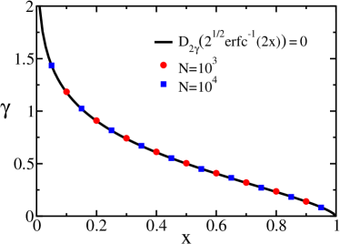
Figure 8: The exponent $\gamma$ versus the scaling variable $x$. The line shows the prediction of the cone approximation given in equation (30), as well as results of numerical simulations with $N=10^{3}$ (bullets) and $N=10^{4}$ particles (squares).

VII Discussion

In summary, we investigated two first-passage problems involving ordered random walks in one dimension. In both cases, there is a series of survival probabilities and a nontrivial family of first-passage exponents. A universal function describes the exponents when the number of particles is very large. Remarkably, there are scaling laws for the scaling exponents.

In general, a first-passage process with $N$ random walks is equivalent to diffusion in a high-dimensional space with a complicated absorbing boundary. This boundary is typically formed by multiple intersecting planes. Solving the first-passage problem is equivalent to solving the electrostatic problem given these boundary conditions bk ; cj ; jdj ; ntv . For example, to find $\beta_{1}=0.228$ for a three-particle system, we must solve for the potential in the exterior of an insulating three-dimensional corner. Yet, the solution, which likely requires an ingenious implementation of the image method, remains unknown even in this physically relevant geometry dr .

To circumvent this difficulty, we introduced the cone approximation in which the absorbing boundary is replaced with the surface of a suitably chosen cone. This approximation is straightforward to implement and utilizes exact and asymptotic properties for first passage in a cone. The cone approximation provides useful estimates for the exponents and moreover, it faithfully captures both typical and extremal features. In particular, the cone approximation yields the correct scaling variable for the first-passage exponents.

We used the term “cone approximation”, yet this framework produces the lower bound whenever the allowed space is a generalized cone with the crucial property of invariance under dilation, ${\bf r}\to a{\bf r}$ cone . The computation of the first-passage exponent in a generalized $d$-dimensional cone requires computation of the lowest eigenvalue $\lambda$ of the angular portion $\nabla^{2}$ of the Laplacian

$$\nabla^{2}f=-\lambda f,$$ (33)

subject to the Dirichlet boundary condition, $f=0$, on the surface of the cone. The choice of the smallest eigenvalue ensures that $f>0$ inside the allowed region. The first-passage exponent $\beta$ is related to the lowest eigenvalue via $\lambda=2\beta(2\beta+d-2)$, see bk .

We now invoke a theorem that, in its simplest form, states that amongst all domains with the same volume, the lowest eigenvalue of the Laplace-Dirichlet operator occurs when the domain is a ball. Rayleigh conjectured this result for two dimensions jwsr , and Faber and Krahn eventually proved it ch . The Rayleigh-Faber-Krahn theorem generalizes to higher dimensions and under mild conditions, to Riemannian manifolds ic . In the context of first-passage processes, this theorem implies that of all generalized cones of fixed solid angle, the first-passage exponent is minimal for the circular cone. Since the regions discussed in our study qualify as generalized cones, results of the cone approximation constitute rigorous lower bounds for the exponents.

Cones can also provide upper bounds. To establish an upper bound, we choose a cone that is inscribed by the absorbing boundary. Clearly, the first-passage process is faster inside the inscribed cone and therefore, the corresponding exponent must be an upper bound.

The cone approximation appears to be asymptotically exact for the leadership problem as it predicts the bulk of the exponents with excellent accuracy. A first step toward proving this exactness is the observation that all opening angles in (26) approach a right angle as the number of particles diverges. The other major challenge is finding an exact, or at least asymptotically exact, framework for calculating the family of exponents in the origin-crossing problem.

Finally, we mention that in the absence of a theoretical method for obtaining statistics of first-passage exactly, Monte Carlo simulations play vital role. We utilized a straightforward simulation technique. It is interesting to find out how accelerated Monte Carlo simulations fare in producing accurate estimates for the exponents dba ; pg ; obdkgs .

This research has been supported by DOE grant DE-AC52-06NA25396 and NSF grant CCF-0829541.

References

- (1) W. Feller, An Introduction to Probability Theory and Its Applications, vol. I (Wiley, New York, 1968).
- (2) G. H. Weiss, Aspects and Applications of the Random Walk (North-Holland, Amsterdam, 1994).
- (3) H. C. Berg, Random Walks in Biology (Princeton University Press, Princeton, 1983).
- (4) J. Rudnick and G. Gaspari, Elements of the Random Walk: An Introduction for Advanced Students and Researchers (Cambridge University, Press, New York, 2004).
- (5) M. E. Fisher, J. Stat. Phys. 34, 667 (1984).
- (6) D. A. Huse and M. E. Fisher, Phys. Rev. B 29, 239 (1984).
- (7) Q. H. Wei, C. Bechinger, and P. Leiderer, Science 287, 625 (2000).
- (8) B. X. Cui, H. Diamant, and B. H. Lin, Phys. Rev. Lett. 89, 188302 (2002).
- (9) B. P. Lee, J. Phys. A 27, 2633 (1994).
- (10) S. Redner, A Guide to First-Passage Processes (Cambridge University Press, New York, 2001).
- (11) B. Derrida, V. Hakim, and V. Pasquier, Phys. Rev. Lett. 75, 751 (1995).
- (12) S. N. Majumdar, Current Science 77, 370 (1999).
- (13) H. Niederhausen, Eur. J. Combinatorics 4, 161 (1983).
- (14) E. Ben-Naim, Z. A. Daya, P. Vorobieff, and R. E. Ecke, Phys. Rev. Lett. 86, 1414 (2001).
- (15) M. E. Fisher and M. P. Gelfand, J. Stat. Phys. 53, 175 (1988).
- (16) M. Bramson and D. Griffeath, in: Random Walks, Brownian Motion, and Interacting Particle Systems: A Festshrift in Honor of Frank Spitzer, eds. R. Durrett and H. Kesten (Birkhäuser, Boston, 1991).
- (17) D. J. Grabiner, Ann. Inst. Poincare: Prob. Stat. 35, 177 (1999).
- (18) P. L. Krapivsky and S. Redner, J. Phys. A 29, 5347 (1996); S. Redner and P. L. Krapivsky, Amer. J. Phys. 67, 1277 (1999).
- (19) D. ben-Avraham, B. M. Johnson, C. A. Monaco, P. L. Krapivsky, and S. Redner, J. Phys. A 36, 1789 (2003).
- (20) J. Cardy and M. Katori, J. Phys. A 36, 609 (2003).
- (21) D. L. Burkholder, Adv. Math. 26, 182 (1977).
- (22) S. B. Yuste, L. Acedo, and K. Lindenberg, Phys. Rev. E 64, 052102 (2001).
- (23) G. I. Barenblatt, Scaling, Self-Similarity, and Intermediate Asymptotics (Cambridge University Press, Cambridge, 1996).
- (24) H. E. Stanley, Introduction to Phase Transitions and Critical Phenomena (Oxford University Press, New York, 1971).
- (25) E. Ben-Naim and P. L. Krapivsky, Kinetics of First Passage in a Cone, preprint.
- (26) T. E. Harris, J. Appl. Prob. 2, 323 (1965).
- (27) D. G. Levitt, Phys. Rev. A 6, 3050 (1973).
- (28) S. Alexander and P. Pincus, Phys. Rev. B. 18, 2011 (1978).
- (29) H. van Beijeren, K. W. Kehr, and R. Kutner, Phys. Rev. B 28, 5711 (1983).
- (30) C. A. Tracy and H. Widom, Commun. Math. Phys. 159, 151 (1994)
- (31) R. Arratia, Ann. Probab. 11, 362 (1983).
- (32) P. L. Krapivsky, S. Redner, and E. Ben-Naim, A Kinetic View of Statistical Physics (Cambridge University Press, Cambridge, 2010).
- (33) R. D. DeBlassie, Probab. Theory Relat. Fields 74, 1 (1987); Probab. Theory Relat. Fields 79, 95 (1988).
- (34) R. Bañuelos and R. G. Smiths, Probab. Theory Relat. Fields 108, 299 (1997).
- (35) NIST Handbook of Mathematical Functions, ed. F. W. J. Olver, D. M. Lozier, et al. (Cambridge University Press, Cambridge, 2010).
- (36) To obtain the largest exponent , we use when . For opening angles , the survival exponent grows linearly with dimension: with .
- (37) E. Ben-Naim and N. W. Hengartner, Phys. Rev. E 76, 026106 (2007).
- (38) D. ben-Avraham, S. N. Majumdar, and S. Redner, J. Stat. Mech. L04002 (2007).
- (39) T. Antal, E. Ben-Naim, and P. L. Krapivsky, J. Stat. Mech. P07009 (2010).
- (40) H. S. Carslaw and J. C. Jaeger, Conduction of Heat in Solids (Clarendon Press, Oxford, 1959).
- (41) J. D. Jackson, Classical Electrodynamics (Wiley, New York, 1998).
- (42) N. Th. Varopoulos, Math. Proc. Camb. Phi. Soc. 125, 335 (1999); Math. Proc. Camb. Phi. Soc. 129, 301 (1999).
- (43) L. C. Davis and J. Reitz, J. Math. Phys. 16, 1219 (1975).
- (44) A generalized cone is an infinite convex domain that contains a special point, called an apex, and has the property that each ray emanating from the apex and going through any point inside a cone lies inside the cone.
- (45) J. W. S. Rayleigh, The Theory of Sound (Macmillan, New York, 1877; reprinted Dover, New York, 1945).
- (46) R. Courant and D. Hilbert, Methods of Mathematical Physics, vol. I (Wiley, New York, 1953).
- (47) I. Chavel, Eigenvalues in Riemannian geometry (Academic Press, Orlando, 1984).
- (48) D. ben-Avraham, J. Chem. Phys. 88, 941 (1988).
- (49) P. Grassberger, Computer Phys. Comm. 147, 64 (2002).
- (50) T. Oppelstrup, V. V. Bulatov, A. Donev, M. H. Kalos, G. H. Gilmer, and B. Sadigh, Phys. Rev. E 80, 066701 (2009).