Kinetics of First Passage in a Cone

Abstract

We study statistics of first passage inside a cone in arbitrary spatial dimension. The probability that a diffusing particle avoids the cone boundary decays algebraically with time. The decay exponent depends on two variables: the opening angle of the cone and the spatial dimension. In four dimensions, we find an explicit expression for the exponent, and in general, we obtain it as a root of a transcendental equation involving associated Legendre functions. At large dimensions, the decay exponent depends on a single scaling variable, while roots of the parabolic cylinder function specify the scaling function. Consequently, the exponent is of order one only if the cone surface is very close to a plane. We also perform asymptotic analysis for extremely thin and extremely wide cones.

I Introduction

Random walks are widely used to model natural processes in physics, chemistry, and biology wf ; ghw ; hcb ; rg . In particular, first-passage and persistence statistics sr ; snm of multiple random walks underlie reaction-diffusion processes kbr , spin systems dhp ; msbc ; dhz , and polymer dynamics bdve ; is .

First-passage processes involving multiple random walks are equivalent to diffusion in a restricted region of space. For example, the probability that $N$ ordinary random walks do not meet is equivalent to the probability that a “compound” walk in $N$ dimensions remains confined to the region $x_{1}<x_{2}<\ldots<x_{N}$. This probability decays as $t^{-N(N-1)/4}$ in the long-time limit mef ; hf ; djg .

When there are only two or three particles, the compound walk is, in many cases, confined to a wedge, formed by two intersecting planes. Moreover, the well-known properties of diffusion inside an absorbing wedge sr explain the long-time kinetics mef ; fg ; dba ; kr ; bjmkr . In general, however, the absorbing boundary is defined by multiple intersecting planes in a high-dimensional space. Apart from a few special cases, diffusion subject to such complicated boundaries conditions remains an open problem hn ; bg ; kr ; bjmkr ; ck .

Our goal is to use cones in high dimensions to approximate the absorbing boundaries that underlie such first-passage processes. In this study, we obtain analytic results for the survival probability of a diffusing particle inside an absorbing cone in arbitrary dimension. In a follow-up study bk , we demonstrate that cones provide useful approximations to first-passage characteristics of multiple random walks yal .

Figure 1: Illustration of a cone with opening angle $\alpha$. The initial location of the particle is parametrized by the radial distance $r$ and the polar angle $\theta$.

We consider a single particle that diffuses inside an unbounded cone with opening angle $\alpha$ in spatial dimension $d$ (Figure 1). The central quantity in our study is the probability $S(t)$ that the particle does not reach the cone boundary up to time $t$. Regardless of the starting position, this survival probability decays algebraically, $S\sim t^{-\beta}$, in the long-time limit.

First, we find the exponent $\beta$ analytically by solving the Laplace equation inside the cone. In dimensions two and four, this exponent is an explicit function of the opening angle $\alpha$, and in particular, $\beta=(\pi-\alpha)/2\alpha$ when $d=4$. In general dimension, we find $\beta$ as a root of a transcendental equation involving the associated Legendre functions.

Second, we derive scaling properties of the exponent. Interestingly, the exponent $\beta$ becomes a function of a single scaling variable in the large-$d$ limit. We obtain the scaling function as a root of the transcendental equation

$$D_{2\beta}(y)=0\quad{\rm with}\quad y=(\cos\alpha)\sqrt{d}$$ (1)

involving the parabolic cylinder function $D_{\nu}$. The exponent $\beta$ is of order one only in a small region around $\alpha=\pi/2$. The width of this region shrinks as $d^{-1/2}$ in the infinite dimension limit. The exponent diverges algebraically, $\beta(y)\simeq y^{2}/8$ as $y\to\infty$, and it is exponentially small, $\beta(y)\simeq\sqrt{y^{2}/8\pi}\exp(-y^{2}/2)$ when $y\to-\infty$. Thus, in the large-$d$ limit, the exponent $\beta$ is huge if the opening angle is acute, and conversely, it is tiny if the opening angle is obtuse. Strikingly, if we fix the opening angle $\alpha$ and take the limit $d\to\infty$, there are three distinct possibilities,

$$\lim_{d\to\infty}\beta_{d}(\alpha)=\begin{cases}\infty&\alpha<\pi/2,\\ 1/2&\alpha=\pi/2,\\ 0&\alpha>\pi/2.\\ \end{cases}$$ (2)

Of course, a cone with opening angle $\alpha=\pi/2$ is simply a plane, and hence, $\beta(\alpha=\pi/2)=1/2$ for all $d$.

Third, we study the limiting cases of very thin and very wide cones. The exponent diverges algebraically, $\beta\sim\alpha^{-1}$, when the cone is extremely thin. When the cone is extremely wide, the exponent is exponentially small, $\beta\sim(\pi-\alpha)^{d-3}$.

The rest of this paper is organized as follows. In Section II, we write the diffusion equation that governs the survival probability, and show that finding the leading asymptotic behavior of the survival probability requires a solution to the Laplace equation rdd ; dz ; bs ; bd ; ntv . We present the solutions to this Laplace equation in two and four dimensions in Section III, and for an arbitrary dimension in Section IV. The bulk of the paper deals with asymptotic analysis for very large dimensions. In particular, we derive scaling properties of the exponent and obtain the limiting behaviors of the scaling function (Section V). Asymptotic results for extremely thin and extremely wide cones are detailed in Sections VI and VII, respectively. We also obtain the first-passage time (Section VIII) and conclude with a discussion in Section IX.

II The Diffusion Equation

Consider a particle undergoing Brownian motion bdup ; mp inside an unbounded cone in spatial dimension $d$. The opening angle $\alpha$, that is, the angle between the cone axis and its surface, fully specifies the cone (Figure 1). The range of opening angles is $0\leq\alpha\leq\pi$, and for $\alpha=\pi/2$, the cone surface is planar. Moreover, the exterior of the cone is itself a cone with opening angle $\pi-\alpha$. In two dimensions, the cone is a wedge, and in three dimensions, the cone is an ordinary circular cone.

At time $t=0$, the particle is released from a certain location inside the cone. Our goal is to determine the probability that the particle does not reach the cone surface up to time $t$. By symmetry, this survival probability, $S\equiv S(r,\theta,t)$, depends on the initial distance to the apex $r$, and the initial angle with the cone axis $\theta$. Using a spherical coordinate system where the origin is located at the cone apex and the $z$-axis is along the cone axis, the pair of parameters $(r,\theta)$ are simply the radial and the polar angle coordinates of the initial location (Figure 1).

The survival probability fully quantifies the first-passage process. For example, the probability that the particle first reaches the cone surface during the time interval $(t,t+dt)$ equals $[-dS(r,\theta,t)/dt]\times dt$. In general, the survival probability satisfies the diffusion equation ghw

$$\frac{\partial S(r,\theta,t)}{\partial t}=D\nabla^{2}S(r,\theta,t),$$ (3)

where $D$ is the diffusion constant. The initial condition is $S(r,\theta,t=0)=1$, and the boundary condition is $S(r,\alpha,t)=S(0,\theta,t)=0$.

We are primarily interested in the large-time kinetics. Based on the behavior in two and three dimensions sr , we expect that the survival probability decays algebraically,

$$S(r,\theta,t)\simeq\,\Phi(r,\theta)\,t^{-\beta},$$ (4)

as $t\to\infty$. The exponent $\beta\equiv\beta_{d}(\alpha)$ depends on the spatial dimension $d$ and the opening angle $\alpha$. The dependence on the initial location enters only through the amplitude $\Phi$.

We now substitute the leading asymptotic behavior (4) into the diffusion equation (3). Since the time derivative becomes negligible in the long-time limit, the amplitude $\Phi$ satisfies Laplace’s equation,

$$\nabla^{2}\Phi(r,\theta)=0,$$ (5)

subject to the boundary conditions $\Phi(r,\alpha)=\Phi(0,\theta)=0$. The survival probability is finite and positive everywhere inside the cone, and consequently, the amplitude must be finite and positive, $0<\Phi(r,\theta)<\infty$ for all $\theta<\alpha$. In addition, $d\Phi/d\theta|_{\theta=0}=0$, to avoid a cusp along the cone axis.

We use dimensional analysis krb to solve Eq. (5). The survival probability is dimensionless, and hence, (4) implies $[\Phi]=T^{\beta}$ where $T$ denotes dimension of time. The amplitude $\Phi$ depends on three variables: the radial coordinate $r$ with dimension of length, $[r]=L$, the diffusion coefficient $D$ with $[D]=L^{2}/T$, and the dimensionless angle $\theta$. As the quantity $(r^{2}/D)^{\beta}$ is the only combination of the variables $r$ and $D$ with dimension $T^{\beta}$, we seek a solution in the form

$$\Phi(r,\theta)=\left(\frac{r^{2}}{D}\right)^{\beta}\psi(\theta).$$ (6)

The angular function $\psi(\theta)$ must be finite and positive everywhere inside the cone, $0<\psi(\theta)<\infty$ for $\theta<\alpha$, and it vanishes on the cone surface, $\psi(\alpha)=0$.

We now write the Laplacian operator in (5) explicitly by using

$$\nabla^{2}\equiv\frac{\partial^{2}}{\partial r^{2}}\!+\!\frac{d\!-\!1}{r}\frac{\partial}{\partial r}\!+\!\frac{1}{r^{2}(\sin\theta)^{d\!-\!2}}\frac{\partial}{\partial\theta}(\sin\theta)^{d\!-\!2}\frac{\partial}{\partial\theta}.$$

Next, we substitute (6) into the Laplace equation and find that the angular function $\psi\equiv\psi(\theta)$ satisfies the eigenvalue equation rdd ; dz ; bs ; bd ; ntv

$$\frac{1}{(\sin\theta)^{d-2}}\frac{d}{d\theta}\left[(\sin\theta)^{d-2}\frac{d\psi}{d\theta}\right]+2\beta(2\beta+d-2)\psi=0.$$ (7)

The boundary conditions are $\psi^{\prime}(0)=0$ and $\psi(\alpha)=0$.

From equations (4) and (6), the leading asymptotic behavior is

$$S(r,\theta,t)\simeq\psi(\theta)\,\left(\frac{D\,t}{r^{2}}\right)^{-\beta},$$ (8)

as $t\to\infty$. In particular, the survival probability grows algebraically with distance, $S\simeq r^{2\beta}$. We note that the problem of finding the leading asymptotic behavior of the survival probability reduces to an electrostatic problem cj ; jdj as the amplitude satisfies Laplace’s equation (5).

Our goal is to find the exponent $\beta$ and the angular function $\psi(\theta)$. We expect that the exponent is a monotonically decreasing function of the opening angle $\alpha$. Also, in all dimensions, $\beta(\alpha=\pi/2)=1/2$ because a cone with opening angle $\alpha=\pi/2$ is a half-space and consequently, the first-passage probability is identical to that of a particle in the vicinity of a trap in one dimension sr .

III Dimensions Two and Four

We first discuss two special cases where explicit solutions are possible. In dimension two, the second order differential equation (7) reads $\psi_{\theta\theta}+(2\beta)^{2}\,\psi=0$, and the two independent solutions are simply $\cos(2\beta\theta)$ and $\sin(2\beta\theta)$. The boundary condition $\psi^{\prime}(0)=0$ excludes the latter and therefore,

$$\psi_{2}(\theta)=\cos(2\beta\theta).$$ (9)

Henceforth, the subscript indicates the dimension. Since the linear equation (7) specifies the angular function only up to an overall constant, we set the prefactor to one throughout this paper. The boundary condition $\psi(\alpha)=0$ and the requirement that the angular function must be positive everywhere inside the cone together imply $2\beta\alpha=\pi/2$. Therefore, the exponent is sr

$$\beta_{2}(\alpha)=\frac{\pi}{4\alpha}.$$ (10)

As expected, the exponent is a monotonically decreasing function of $\alpha$, and $\beta_{2}(\pi/2)=1/2$. The exponent is minimal, yet finite, $\beta_{2}(\pi)=1/4$, for an absorbing needle cr . Thus, in dimension two, a diffusing particle reaches a needle with certainty.

In dimension four, the transformation $\psi_{4}(\theta)=(\sin\theta)^{-1}u(\theta)$ reduces the eigenvalue equation (7) to $u_{\theta\theta}+(2\beta+1)^{2}u=0$. Now, the two independent solutions are $\sin[(2\beta+1)\theta]$ and $\cos[(2\beta+1)\theta]$, but the latter is forbidden because the function $\psi$ must be finite. Therefore,

$$\psi_{4}(\theta)=\frac{\sin\left[(2\beta+1)\theta\right]}{\sin\theta}.$$ (11)

The boundary condition $\psi(\alpha)=0$ and the requirement $\psi(\theta)>0$ for $\theta<\alpha$ together give $(2\beta+1)\alpha=\pi$. Hence, the exponent is an explicit function of the opening angle in dimension four as well,

$$\beta_{4}(\alpha)=\frac{\pi-\alpha}{2\alpha}.$$ (12)

The exponent vanishes, $\beta_{4}(\alpha)\to 0$ as $\alpha\to\pi$, so it is no longer guaranteed that a diffusing particle reaches a needle.

IV General Dimension

In general dimension, we transform the eigenvalue equation (7) using the variable $\mu=\cos\theta$. In terms of this variable, the function $\psi\equiv\psi_{d}(\mu)$ satisfies

$$(1-\mu^{2})\frac{d^{2}\psi}{d\mu^{2}}-(d-1)\,\mu\,\frac{d\psi}{d\mu}+2\beta(2\beta+d-2)\psi=0.$$ (13)

The boundary condition is $\psi(\cos\alpha)=0$. We now use a second transformation,

$$\psi(\mu)=\left(1-\mu^{2}\right)^{-\delta/2}\!\Psi(\mu)\quad{\rm with}\quad\delta=\frac{d-3}{2}.$$

Substituting this form into (13) shows that the auxiliary function $\Psi\equiv\Psi_{d}(\mu)$ satisfies the associated Legendre equation as ; NIST

$$(1-\mu^{2})\frac{d^{2}\Psi}{d\mu^{2}} - 2\,\mu\,\frac{d\Psi}{d\mu}$$

$$+ \left[(2\beta+\delta)(2\beta+\delta+1)-\frac{\delta^{2}}{1-\mu^{2}}\right]\Psi=0.$$

The two independent solutions of this equation are $P_{2\beta+\delta}^{\delta}(\mu)$ and $Q_{2\beta+\delta}^{\delta}(\mu)$, the associated Legendre functions of degree $2\beta+\delta$ and order $\delta$. In even dimensions, the first solution is not physical because it implies a divergence of $\psi$ as $\theta\to 0$ NIST . In odd dimensions, the second solution is excluded for the same reason. Therefore note ,

$$\psi_{d}(\theta)=\begin{cases}(\sin\theta)^{-\delta}P_{2\beta+\delta}^{\delta}(\cos\theta)&d\ {\rm odd},\\ (\sin\theta)^{-\delta}Q_{2\beta+\delta}^{\delta}(\cos\theta)&d\ {\rm even}.\end{cases}$$ (15)

The boundary condition $\psi(\alpha)=0$ relates the exponent $\beta$ and the opening angle $\alpha$,

$$\begin{split}P_{2\beta+\delta}^{\delta}(\cos\alpha)&=0\qquad d\ {\rm odd},\\ Q_{2\beta+\delta}^{\delta}(\cos\alpha)&=0\qquad d\ {\rm even}.\end{split}$$ (16)

In general dimension, the exponent $\beta$ is the smallest root of the transcendental equation (16) involving the associated Legendre functions. We must always choose the smallest root because $\psi(\theta)>0$ for all $\theta<\alpha$.

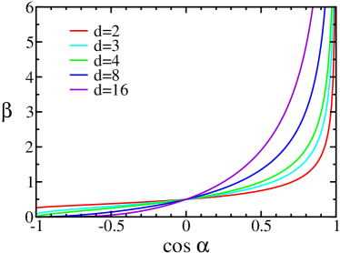
Figure 2: The survival exponent $\beta$ versus $\cos\alpha$ at different dimensions. This exponent is given explicitly by (10) and (12) in dimensions $d=2$ and $d=4$, respectively. In general, the exponent is a root of the transcendental equation (16).

We can verify that the exponent $\beta$ decreases monotonically with the opening angle $\alpha$, and that $\beta(\pi/2)=1/2$ (Figure 2). In all dimensions, the exponent diverges for extremely thin cones, $\alpha\to 0$, and when $d\geq 3$, the exponent vanishes when $\alpha\to\pi$.

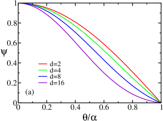
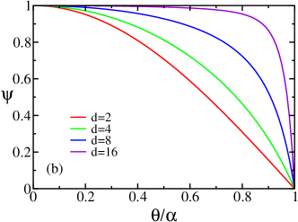
Figure 3: The function $\psi(\theta)$ versus the normalized polar angle $\theta/\alpha$ at different dimensions. The function $\psi(\theta)$ is normalized such that $\psi(0)=1$. Figure 3a shows the behavior for an acute opening angle, $\alpha=\pi/4$, and Figure 3b shows the behavior for an obtuse opening angle, $\alpha=3\pi/4$.

Let us fix the opening angle and increase the dimension. There are two possibilities: (i) if $\alpha<\pi/2$, the first-passage process speeds up with increasing dimension because $\beta$ increases (Figure 2) and $\psi(\theta)$ declines (Figure 3a); (ii) if $\alpha>\pi/2$, the first-passage process slows down because $\beta$ shrinks (Figure 2) and $\psi(\theta)$ grows (Figure 3b). Ultimately, in the infinite-dimension limit, first passage becomes instantaneous for acute angles but infinitely long for obtuse angles.

In dimension three, $\delta=0$, and the solution (15) reduces to the Legendre function of index $2\beta$, namely, $\psi_{3}(\theta)=P_{2\beta}(\cos\theta)$ as ; NIST . Also, the exponent $\beta$ is the smallest root of the transcendental equation sr

$$P_{2\beta}(\cos\alpha)=0.$$ (17)

For half-integer values of the exponent, $\beta=n/2$, the angular function $\psi_{d}(\theta)$ is a polynomial of degree $n$ in $\cos\theta$. This follows directly from equation (13). For example,

$$\psi_{d}(\theta)=\begin{cases}\cos\theta&\beta=1/2,\\ d\cos^{2}\theta-1&\beta=1,\\ (d+2)\cos^{3}\theta-3\cos\theta&\beta=3/2.\end{cases}$$ (18)

In three dimensions, the polynomials coincide with the Legendre polynomials: $\psi_{3}(\theta)=P_{n}(\cos\theta)$ when $\beta=n/2$. Using $\psi(\alpha)=0$, we find the opening angles for which the exponent is a half-integer:

$${\beta}_{d}(\alpha)=\begin{cases}1/2\quad&\cos\alpha=0,\\ 1\quad&\cos\alpha=1/\sqrt{d},\\ 3/2\quad&\cos\alpha=\sqrt{3/(d+2)}.\end{cases}$$ (19)

V Scaling Properties

The special values listed in (19) suggest that the survival exponent has the scaling form

$$\beta_{d}(\alpha)\to\beta(y)\quad{\rm with}\quad y=(\cos\alpha)\sqrt{d},$$ (20)

in the limit $d\to\infty$. From equation (19), we deduce $\beta(y=0)=1/2$, $\beta(y=1)=1$, and $\beta(y=\sqrt{3})=3/2$. To show the scaling behavior (20) in general, we introduce the variable $z=\mu\,\sqrt{d}$. Performing this scaling transformation on the Laplace equation (13) shows that the angular function depends on a single scaling variable, $\psi_{d}(\mu)\to\psi(z)$, in the $d\to\infty$ limit. The scaling function $\psi(z)$ satisfies

$$\psi_{zz}-z\,\psi_{z}+2\beta\psi=0.$$ (21)

The boundary condition is $\psi(z=y)=0$, and additionally, $\psi(z)>0$ for all $y<z<\infty$.

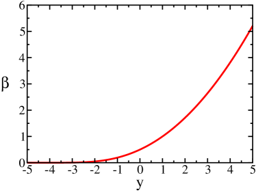
Figure 4: The exponent $\beta$, specified by equation (23), versus the scaling variable $y=(\cos\alpha)\sqrt{d}$.

Using the transformation $\psi(z)=\exp(z^{2}/4)u(z)$, we recast (21) into the parabolic cylinder equation bo

$$u_{zz}+\left(2\beta+\frac{1}{2}-\frac{z^{2}}{4}\right)u=0.$$

The two independent solutions of this equation are $D_{2\beta}(z)$ and $D_{2\beta}(-z)$ where $D_{\nu}(z)$ is the parabolic cylinder function of index $\nu$. The second solution is not physical: the asymptotic behavior $D_{\nu}(-z)\sim\exp(z^{2}/4)$ as $z\to\infty$ bo implies a divergent survival probability in the limit $\theta\to 0$. Therefore,

$$\psi(z)=e^{z^{2}/4}D_{2\beta}(z).$$ (22)

As always, we set the overall proportionality constant to one. The boundary condition $\psi(z=y)=0$ relates the scaling function $\beta(y)$ and the scaling variable $y$, defined in (20),

$$D_{2\beta}(y)=0.$$ (23)

The proper solution is the largest root of the parabolic cylinder function. For half-integer values of the exponent, the parabolic cylinder function is related to a Hermite polynomial, $D_{2\beta}(z)\propto H_{n}(z/\sqrt{2})\exp(-z^{2}/4)$, and hence, (23) is equivalent to $H_{n}(y/\sqrt{2})=0$, where the largest root is the appropriate one. Therefore, the half-integer values of the scaling function $\beta(y)$ occur at zeroes of Hermite polynomials. In addition to the aforementioned values, we also quote $\beta\big{(}\sqrt{3+\sqrt{6}}\,\big{)}=2$ and $\beta\big{(}\sqrt{5+\sqrt{10}}\,\big{)}=5/2$.

The scaling behavior (20) is valid in the limits $\alpha\to\pi/2$ and $d\to\infty$ with the scaling variable $y=(\cos\alpha)\sqrt{d}$ or alternatively $y=(\pi/2-\alpha)\sqrt{d}$ kept finite. Hence, the scaling function in (23) quantifies the shape of $\beta$ in a “scaling window” bbckw ; bk1 ; abk centered on $\alpha=\pi/2$. The size of this window shrinks as $d^{-1/2}$ at large dimensions. As shown in Figure 4, $\beta$ vanishes as $y\to-\infty$, and it diverges as $y\to\infty$. Surprisingly, if we fix the opening angle $\alpha$ and then take the $d\to\infty$ limit, there are three distinct possibilities, as stated in (2): the exponent vanishes if $\alpha>\pi/2$, it always equals $1/2$ when $\alpha=\pi/2$, and it diverges if $\alpha<\pi/2$.

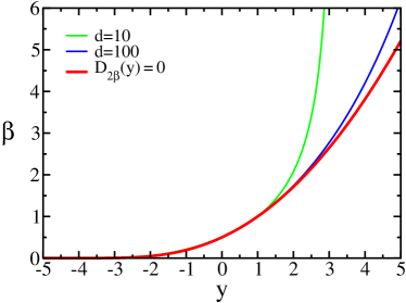
Figure 5: The convergence to the scaling behavior. The exponent $\beta\equiv\beta_{d}(\alpha)$, specified by (16), is plotted versus the scaling variable $y=(\cos\alpha)\sqrt{d}$ for $d=10$ and $d=100$. Also shown is the scaling function $\beta(y)$.

We also note that the approach to the scaling behavior is not uniform. The scaling exponent $\beta$ converges rapidly to the scaling function for negative $y$, but the convergence is quite slow for positive $y$ (Figure 5).

To find the asymptotic behavior when $y\to\infty$, we use the fact that the largest root $\xi\equiv\xi(\nu)$ of the parabolic cylinder function of index $\nu$, $D_{\nu}(\xi)=0$, is located at as

$$\xi\simeq(4\nu)^{1/2}-|a_{1}|\,\nu^{-1/6},$$

when $\nu\to\infty$. Here, $a_{1}\cong-2.338107$ is the first root of the Airy function. Substituting $\nu=2\beta$ into this expression, we find $y\simeq(8\beta)^{1/2}-|a_{1}|(2\beta)^{-1/6}$ as $\beta\to\infty$. Therefore, the leading behavior is $\beta\simeq y^{2}/8$. Furthermore, the first correction to this asymptotic form is

$$\beta\simeq\frac{y^{2}}{8}+|a_{1}|2^{-5/3}\,y^{2/3}.$$ (24)

Thus, the exponent $\beta$ diverges algebraically when $y\to\infty$.

We use perturbation analysis to find how $\beta$ vanishes in the complementary limit $y\to\infty$. Equation (21) shows that the angular function becomes constant when $\beta\to 0$. Thus, $\psi(z)\simeq 1+\beta\,g(z)$. Substituting this form into (21), the correction function $g\equiv g(z)$ obeys

$$g_{zz}-zg_{z}+2=0.$$ (25)

The boundary condition

$$g_{z}(0)=\sqrt{2\pi}$$ (26)

follows from the small-$\beta$, small-$z$, behavior of the scaling solution (22)

$$\psi(z)\simeq 1+\frac{D_{2\beta}^{\prime}(0)}{D_{2\beta}(0)}\,z=1-\frac{\sqrt{2}\,\Gamma(\tfrac{1}{2}-\beta)}{\Gamma(-\beta)}\,z\simeq 1+\sqrt{2\pi}\,\beta\,z.$$

Here, we used the values $D_{2\beta}(0)=\sqrt{\pi}\,2^{\beta}/\Gamma(1/2-\beta)$ and $D_{2\beta}^{\prime}(0)=-\sqrt{\pi}\,2^{\beta+1/2}/\Gamma(-\beta)$ bo , as well as the identities $\Gamma(1/2)=\sqrt{\pi}$ and $(-\beta)\Gamma(-\beta)=\Gamma(1-\beta)$.

Using the integrating factor $I(z)=\exp(-z^{2}/4)$, we simplify Eq. (25) to $d(g_{z}\,I)/dz=-2I$. Integration of this equation subject to the boundary condition (26) gives

$$g(z)=2\int_{0}^{z}dt\,e^{t^{2}/2}\int_{t}^{\infty}ds\,e^{-s^{2}/2}.$$ (27)

The second integral approaches a constant, and consequently, $g(z)\simeq-\sqrt{8\pi/z^{2}}\exp(z^{2}/2)$, when $z\to-\infty$. We now impose the boundary condition $\psi(y)=1+\beta\,g(y)=0$, and find that the exponent is exponentially small,

$$\beta(y)\simeq\sqrt{\frac{y^{2}}{8\pi}}\,e^{-y^{2}/2},$$ (28)

in the limit $y\to-\infty$.

In summary, the scaling function $\beta(y)$ has the following extremal behaviors

$$\beta(y)\simeq\begin{cases}\sqrt{y^{2}/8\pi}\,\exp\!\left(-y^{2}/2\right)&y\to-\infty,\\ y^{2}/8&y\to\infty.\end{cases}$$ (29)

At large dimensions, these limiting behaviors apply only inside the scaling window, that is, when $|\pi/2-\alpha|$ is of the order $d^{-1/2}$. In the next two sections, we perform asymptotic analysis for the limiting cases of extremely thin cones ($\theta\to 0$) and extremely wide cones ($\theta\to\pi)$.

VI Thin Cones

The explicit expressions (10) and (12) show that the exponent is inversely proportional to the opening angle, $\beta\sim\alpha^{-1}$, when the cone is extremely thin. We anticipate that this divergence is generic.

When the cone is very thin, we have $\sin\theta\simeq\theta$ and equation (7) simplifies,

$$\frac{d^{2}\psi}{d\theta^{2}}+\frac{d-2}{\theta}\,\frac{d\psi}{d\theta}+(2\beta)^{2}\psi=0.$$ (30)

This equation holds as long as $d\alpha^{2}\ll 1$. In writing this equation we tacitly assumed a divergent $\beta$. We now introduce the scaling variable $x=2\beta\theta$ and transform equation (30) as follows,

$$\psi_{xx}+\frac{d-2}{x}\,\psi_{x}+\psi=0.$$

Next, we seek a solution in the form $\psi(x)=x^{-\delta}u(x)$, where as in (15), $\delta=\frac{d-3}{2}$. Performing this second transformation gives the Bessel equation jdw

$$x^{2}\,u_{xx}+x\,u_{x}+\left(x^{2}-\delta^{2}\right)u=0.$$

This equation has two independent solutions: the Bessel functions $J_{\delta}(x)$ and $Y_{\delta}(x)$. The boundary condition $\psi^{\prime}(0)=0$ excludes the latter and hence,

$$\psi(x)=x^{-\delta}J_{\delta}(x).$$ (31)

The other boundary condition, $\psi(\alpha)=0$, gives an implicit relation $J_{\delta}(2\beta\alpha)=0$ between the exponent $\beta$ and the opening angle $\alpha$. We see that the exponent is inversely proportional to the opening angle in all dimensions:

$$\beta_{d}(\alpha)\simeq B_{d}\,\alpha^{-1}\quad{\rm with}\quad B_{d}=\tfrac{1}{2}\zeta(\delta),$$ (32)

as $\alpha\to 0$. Here, $\zeta(\delta)$ is the first positive zero of the Bessel function, $J_{\delta}(\zeta)=0$. Table I lists the coefficients $B_{d}$ for $d\leq 10$.

$d$	$B_{d}$
$2$	$0.785398$
$3$	$1.202412$
$4$	$1.570796$
$5$	$1.915852$
$6$	$2.246704$
$7$	$2.567811$
$8$	$2.881729$
$9$	$3.190080$
$10$	$3.493966$

Table 1: The coefficient $B_{d}$ in (32) for $d\leq 10$. Equations (9) and (11) yield $B_{2}=\pi/4$ and $B_{4}=\pi/2$, respectively.

At large dimensions, we use the asymptotic behavior as ; NIST

$$\zeta(\delta)\simeq\delta+|a_{1}|(\delta/2)^{1/3}$$

when $\delta\to\infty$. Again, $a_{1}\cong-2.338107$ is the first root of the Airy function. Thus, to leading order, the prefactor $B_{d}$ is linear in the dimension, $B_{d}\simeq d/4$. The correction to the leading asymptotic behavior is given by

$$B_{d}\simeq\frac{d}{4}+|a_{1}|2^{-5/3}d^{1/3},$$ (33)

for $d\to\infty$. The divergence (32) shows that a diffusing particle quickly reaches the cone surface when the cone is thin. Moreover, equation (33) implies $\beta\simeq d/4\alpha$, and hence, the first-passage process becomes even faster as the dimension increases.

VII Wide Cones

For all $d\geq 3$, the solutions to equation (16) show that the exponent vanishes when the interior of the cone occupies all of space (Figure 2). In this case, equation (7) becomes

$$\frac{1}{(\sin\theta)^{d-2}}\frac{d}{d\theta}\left[(\sin\theta)^{d-2}\frac{d\psi}{d\theta}\right]+2\beta(d-2)\psi=0.$$ (34)

We obtain $\beta$ by repeating the perturbation analysis leading to (28). For all $d\geq 3$, we write $\psi(\theta)\simeq 1+\beta\,g(\theta)$. The boundary condition $\psi^{\prime}(0)=0$ implies $g^{\prime}(0)=0$. From (34), the correction $g\equiv g(\theta)$ obeys

$$\frac{d}{d\theta}\left[(\sin\theta)^{d-2}\frac{dg}{d\theta}\right]=-2(d-2)(\sin\theta)^{d-2}.$$ (35)

Integrating this equation twice and using the boundary condition $g^{\prime}(0)=0$, we find the correction up to a constant,

$$g(\theta)=g_{0}-2(d\!-\!2)\!\int_{0}^{\theta}\!\!\!\frac{d\phi}{(\sin\phi)^{d-2}}\int_{0}^{\phi}\!\!d\varphi\,(\sin\varphi)^{d-2}.$$ (36)

In the limit $\theta\to\pi$, the second integral approaches the constant

$$S_{d}=\int_{0}^{\pi}d\theta\,(\sin\theta)^{d-2}=\frac{\Gamma\left(\tfrac{d-1}{2}\right)\Gamma\left(\tfrac{1}{2}\right)}{\Gamma\left(\tfrac{d}{2}\right)}.$$

Moreover, the term $(\sin\phi)^{-(d-2)}\simeq(\pi-\phi)^{-(d-2)}$ dominates the first integral and therefore, the correction function diverges,

$$g(\theta)\simeq-\frac{2(d-2)S_{d}}{d-3}(\pi-\theta)^{-(d-3)},$$

as $\theta\to\pi$. We now impose the boundary condition $\psi(\alpha)=1+\beta g(\alpha)=0$ and find that the exponent $\beta$ vanishes exponentially as $\alpha\to\pi$,

$$\beta_{d}(\alpha)\simeq A_{d}\,(\pi-\alpha)^{d-3}.$$ (37)

The coefficient $A_{d}=\frac{d-3}{2(d-2)S_{d}}$ is given by

$$A_{d}=\frac{\Gamma\left(\tfrac{d-2}{2}\right)}{2\,\Gamma\left(\tfrac{1}{2}\right)\Gamma\left(\tfrac{d-3}{2}\right)}.$$ (38)

In particular $A_{4}=1/2\pi$, in agreement with equation (12). Table II lists the coefficients $A_{d}$ for $d\leq 10$. The asymptotic property $\Gamma(x+a)/\Gamma(x)\to x^{a}$ as $x\to\infty$ shows that the coefficient grows algebraically with dimension, $A_{d}\simeq\sqrt{d/8\pi}$.

$d$	$3$	$4$	$5$	$6$	$7$	$8$	$9$	$10$
$A_{d}$	$\ 0\$	$\ \frac{1}{2\pi}$	$\ \frac{1}{4}\$	$\ \frac{1}{\pi}\$	$\ \frac{3}{8}\$	$\ \frac{4}{3\pi}\$	$\ \frac{15}{32}\$	$\ \frac{8}{5\pi}\$

Table 2: The coefficient $A_{d}$ given by equation (38) for $d\leq 10$.

In the marginal case $d=3$, the coefficient in (37) vanishes, $A_{3}=0$. In this case, the exponent vanishes gently,

$$\beta_{3}\simeq\frac{1}{4\ln\frac{2}{\pi-\alpha}}$$ (39)

as follows from (17) jdw . This behavior is consistent with the near-$\pi$ behavior of (36), $g(\theta)\simeq-4\ln\frac{1}{\pi-\theta}$.

As the opening angle approaches its maximal value, the cone surface turns into an infinitely long, yet infinitesimally thin needle. In two dimensions, a diffusing particle is bound to reach such a needle. Yet, in dimensions three and higher, the particle may or may not reach the needle. Moreover, the exponentially small exponent (37) shows that the first-passage process becomes extremely slow at high dimensions.

VIII First-Passage Time

We now briefly discuss the first-passage time. Let $T(r,\theta)$ be the average duration of the first-passage process, namely, the average time it takes a particle released at $(r,\theta)$ to reach the cone surface for the first time (Figure 1). This quantity obeys the Poisson equation sr

$$D\nabla^{2}T(r,\theta)=-1,$$ (40)

and the boundary condition $T(r,\alpha)=T(0,\theta)=0$. As in (6), we use dimensional analysis and write $T(r,\theta)=(r^{2}/D)\,U(\theta)$ where $U(\theta)$ is a dimensionless function of the angle. From Eq. (40), we get

$$\frac{1}{(\sin\theta)^{d-2}}\frac{d}{d\theta}\left[(\sin\theta)^{d-2}\frac{dU}{d\theta}\right]+2dU=-1,$$ (41)

while the boundary condition becomes $U(\alpha)=0$. The linear equation (41) has the particular solution $\tilde{U}=-1/2d$, and thus, we seek a solution in the form $U(\theta)=u(\theta)-1/2d$. The function $u\equiv u(\theta)$ obeys the homogeneous linear differential equation

$$\frac{1}{(\sin\theta)^{d-2}}\frac{d}{d\theta}\left[(\sin\theta)^{d-2}\frac{du}{d\theta}\right]+2du=0,$$

subject to the boundary condition $u(\alpha)=1/2d$. This equation is a special case of (7), and using (18), we immediately find $u(\theta)=C(d\cos^{2}\theta-1)$ where $C$ is set by the boundary condition. Finally, we find that the first-passage time has the compact form

$$T(r,\theta)=\frac{r^{2}}{2D}\,\frac{\cos^{2}\theta-\cos^{2}\alpha}{d\cos^{2}\alpha-1}.$$ (42)

This first-passage time is finite if and only if $\beta>1$.

IX Discussion

In summary, we studied first-passage kinetics for a particle diffusing in a cone. In all dimensions, the probability that the particle does not reach the cone boundary decays algebraically with time. We found the exponent underlying this power-law behavior as a root of a transcendental equation involving associated Legendre functions. We also obtained scaling and extremal properties of the exponent.

Our results generalize the known properties of first passage in two- and three-dimensional cones sr to arbitrary dimensions. Moreover, the statistical physics perspective, where scaling plays a central role, extends rigorous studies of diffusion in cones in probability theory rdd ; dz ; bs ; bd and potential theory ntv . Scaling implies that the behavior in a narrow window becomes universal: cones with different combinations of $\alpha$ and $d$, have the same exponent $\beta$, as long as the scaling variable $y=(\cos\alpha)\sqrt{d}$ is the same. The exponent is exponentially small when $y\to-\infty$, and it grows algebraically when $y\to\infty$.

As the dimension increases, the first-passage process speeds up if the opening angle is acute but slows down if the opening angle is obtuse. This behavior is reflected by the asymptotic behavior for fixed $\theta$ in the large-$d$ limit. We merely quote the results of the corresponding asymptotic analysis,

$$\beta_{d}(\alpha)\simeq\begin{cases}\frac{d}{4}\left(\frac{1}{\sin\alpha}-1\right)&\alpha<\pi/2,\\ C(\sin\alpha)^{d}&\alpha>\pi/2.\end{cases}$$ (43)

The exponent is proportional to the dimension at acute angles, and it decays exponentially with dimension at obtuse angles. The asymptotic behavior (43) is consistent with the limiting behavior of the scaling function (29) as well as the asymptotic results (32) and (37).

Kinetics of first-passage in a cone provide useful information about first-passage problems involving multiple random walks. For example, let us consider the random-walk problem mentioned in the introduction. The probability that the trajectories of $N$ ordinary random walks do not meet up to time $t$ is equivalent to the probability that a compound random walk in $N$ dimensions remains inside the region $x_{1}<x_{2}<\cdots<x_{N}$. Since there are $N!$ permutations of the positions, the total solid angle inside this “allowed region” accounts for a fraction $1/N!$ of space. We replace the allowed region with an $N$-dimensional cone that has the same solid angle, $\alpha^{N-1}\sim 1/N!$. Using the Stirling formula, $N!\sim\sqrt{2\pi N}(N/e)^{N}$, the opening angle is $\alpha\simeq e/N$. The survival probability decays algebraically, $S(t)\sim t^{-\beta_{N}}$, and using (32)–(33), the exponent is $\beta_{N}\simeq N^{2}/4e$. This cone approximation correctly gives the asymptotic $N$-dependence as the exact exponent is $N(N-1)/4$ mef ; hf ; djg .

First passage in the exterior of this narrow cone gives an approximation for the probability that the order of $N$ random walks does not turn into the mirror image of the initial state. If the initial ordering of the random walks is $\{1,2,\cdots,N-1,N\}$, then $S(t)$ is the probability that the particles do not reach the configuration $\{N,N-1,\ldots,2,1\}$ up to time $t$. Since the angle of the cone is now $\pi-\alpha\simeq e/N$, the asymptotic behavior (37) gives $S(t)\sim t^{-\beta_{N}}$ with the tiny exponent

$$\beta_{N}\simeq\sqrt{N/8\pi}\,(e/N)^{N-3}.$$

In a follow-up study, we use cones to understand other random walk problems bk .

With a few exceptions such as paraboloids bds ; ls , the study of first passage in elementary geometries is still in its infancy. We considered first passage in basic circular cones. A natural extension is to generalized cones dlb , defined as domains with the property that all rays emanating from the apex do not intersect the cone boundary. Understanding first-passage properties in such generalized cones ultimately requires a solution to the Laplace-Dirichlet boundary value problem.

We thank Sidney Redner for useful discussions. This research has been supported by DOE grant DE-AC52-06NA25396 and NSF grant CCF-0829541.

References

- (1) W. Feller, An Introduction to Probability Theory and Its Applications, (Wiley, New York, 1968).
- (2) G. H. Weiss, Aspects and Applications of the Random Walk (North-Holland, Amsterdam, 1994).
- (3) H. C. Berg, Random Walks in Biology (Princeton University Press, Princeton, 1983).
- (4) J. Rudnick and G. Gaspari, Elements of the Random Walk: An Introduction for Advanced Students and Researchers (Cambridge University, Press, New York, 2004).
- (5) S. Redner, A Guide to First-Passage Processes (Cambridge University Press, New York, 2001).
- (6) S. N. Majumdar, Current Science 77, 370 (1999).
- (7) P. L. Krapivsky, E. Ben-Naim, and S. Redner, Phys. Rev. E 50, 2474 (1994).
- (8) B. Derrida, V. Hakim, and V. Pasquier, Phys. Rev. Lett. 75, 751 (1995).
- (9) S. N. Majumdar, C. Sire, A. J. Bray, and S. J. Cornell, Phys. Rev. Lett. 77, 2867 (1996).
- (10) B. Derrida, V. Hakim, and V. Pasquier, Phys. Rev. Lett. 77, 2871 (1996).
- (11) E. Ben-Naim, Z. A. Daya, P. Vorobieff, and R. E. Ecke, Phys. Rev. Lett. 86, 1414 (2001).
- (12) I. Sokolov, Phys. Rev. Lett. 90, 080601 (2003).
- (13) M. E. Fisher, J. Stat. Phys. 34, 667 (1984).
- (14) D. A. Huse and M. E. Fisher, Phys. Rev. B 29, 239 (1984).
- (15) D. J. Grabiner, Ann. Inst. Poincare: Prob. Stat. 35, 177 (1999).
- (16) D. ben-Avraham, J. Chem. Phys. 88, 941 (1988).
- (17) M. E. Fisher and M. P. Gelfand, J. Stat. Phys. 53, 175 (1988).
- (18) P. L. Krapivsky and S. Redner, J. Phys. A 29, 5347 (1996); S. Redner and P. L. Krapivsky, Amer. J. Phys. 67, 1277 (1999).
- (19) D. ben-Avraham, B. M. Johnson, C. A. Monaco, P. L. Krapivsky, and S. Redner, J. Phys. A 36, 1789 (2003).
- (20) J. Cardy and M. Katori, J. Phys. A 36, 609 (2003).
- (21) H. Niederhausen, Eur. J. Combinatorics 4, 161 (1983).
- (22) M. Bramson and D. Griffeath, in: Random Walks, Brownian Motion, and Interacting Particle Systems: A Festshrift in Honor of Frank Spitzer, eds. R. Durrett and H. Kesten (Birkhäuser, Boston, 1991).
- (23) E. Ben-Naim and P. L. Krapivsky, First-Passage Exponents of Multiple Random Walks, preprint.
- (24) S. B. Yuste, L. Acedo, and Katja Lindenberg, Phys. Rev. E 64, 052102 (2001).
- (25) R. D. DeBlassie, Probab. Theory Relat. Fields 74, 1 (1987); Probab. Theory Relat. Fields 79, 95 (1988).
- (26) B. Davis and B. Zhang, Proc. AMS 121, 925 (1994).
- (27) R. Bañuelos and R. G. Smiths, Probab. Theory Relat. Fields 108, 299 (1997).
- (28) R. Bañuelos and R. D. DeBlassie, Stoch. Proc. Appl. 116, 36 (2006).
- (29) N. Th. Varopoulos, Math. Proc. Camb. Phi. Soc. 125, 335 (1999); Math. Proc. Camb. Phi. Soc. 129, 301 (1999).
- (30) B. Duplantier, in: Einstein, 1905-2005, eds. Th. Damour, O. Darrigol, B. Duplantier and V. Rivasseau (Birkhäuser Verlag, Basel, 2006); arXiv:0705.1951.
- (31) P. Mörders and Y. Peres, Brownian Motion, http://www.stat.berkeley.edu/users/peres/bmbook.pdf.
- (32) P. L. Krapivsky, S. Redner and E. Ben-Naim, A Kinetic View of Statistical Physics (Cambridge University Press, Cambridge, 2010).
- (33) H. S. Carslaw and J. C. Jaeger, Conduction of Heat in Solids (Clarendon Press, Oxford, 1959).
- (34) J. D. Jackson, Classical Electrodynamics (Wiley, New York, 1998).
- (35) D. Considine and S. Redner, J. Phys. A 22, 1621 (1889).
- (36) M. Abramowitz and I. A. Stegun, Handbook of Mathematical Functions (Dover Publications Inc., 1965).
- (37) NIST Handbook of Mathematical Functions, ed. F. W. J. Olver, D. M. Lozier, et al. (Cambridge University Press, Cambridge, 2010).
- (38) The solution holds for all .
- (39) C. M. Bender and S. A. Orszag, Advanced Mathematical Methods for Scientists and Engineers (McGraw-Hill, New York, 1978).
- (40) B. Bollobás, C. Borgs, J. T. Chayes, J. H. Kim, and D. B. Wilson, Rand. Struct. Alg. 18, 201 (2001).
- (41) E. Ben-Naim and P. L. Krapivsky, Phys. Rev. E 71, 026129 (1995)
- (42) T. Antal, E. Ben-Naim, and P. L. Krapivsky, J. Stat. Mech. P07009 (2010).
- (43) J. D. Watson, A Treatise on the Theory of Bessel Functions (Cambridge University Press, Cambridge, 1995).
- (44) R. Bañuelos, R. D. DeBlassie, and R. G. Smiths, Ann. Probab. 29, 882 (2001).
- (45) M. Lifshits and Z. Shi, Bernoulli 8, 745 (2002).
- (46) D. L. Burkholder, Adv. Math. 26, 182 (1977).