The Degrees of Freedom of MIMO Interference Channels without State Information at Transmitters

Abstract

This paper fully determines the degree-of-freedom (DoF) region of two-user interference channels with arbitrary number of transmit and receive antennas in the case of isotropic and independent (or block-wise independent) fading, where the channel state information is available to the receivers but not to the transmitters. The result characterizes the capacity region to the first order of the logarithm of the signal-to-noise ratio (SNR) in the high-SNR regime. The DoF region is achieved using random Gaussian codebooks independent of the channel states, which implies that it is impossible to increase the DoF using beamforming and interference alignment in the absence of channel state information at the transmitters.

I Introduction

The interference channel is one of the most important models for the physical layer of wireless networks. Some recent breakthroughs in understanding the fundamental limits of such channels, with or without multiple antennas are reported in [1, 2, 3, 4, 5]. Most existing studies of interference channels assume that full channel state information (CSI) is available to all transmitters and receivers. In practice, however, the state of the channel is usually measured at the receivers, and it is often difficult for the transmitters to acquire the CSI accurately in a timely manner.

This paper studies a two-user multiple-input multiple-output (MIMO) interference channel subject to isotropic fading, where the channel state is independent over time, and its realization is known to the receivers but not to the transmitters. The channel model is described in Section II. An example of the channel is illustrated in Fig. 1. The degree-of-freedom (DoF) region of the MIMO interference channel is completely characterized by Theorem 1 in Section III. This is the main result in this paper. The result indicates that without CSI at the transmitters (CSIT), no additional gains in terms of DoF can be achieved using beamforming or interference alignment, which is in contrast to the results for the case with full CSI shown in [6]. A detailed proof Theorem 1 is developed in Sections III and IV.

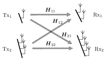
Figure 1: A two-user MIMO interference channel.

Related works [7, 8, 9, 10, 11, 12] also consider interference channels without CSIT. The case of slow fading is modeled as compound interference channels in [7, 8], where the capacity of a single-antenna two-user interference channel is studied in [7], and the diversity-multiplex trade-off of the same model is studied in [8]. In the case of fast (independent) fading, Akuiyibo et al [9] derived an outer bound of capacity region for two-user MIMO interference channels with Rayleigh fading, which is tight in terms of the DoF in some special cases. Tighter outer bounds on the DoF region have been developed by Huang et al in [10], who also assume Rayleigh fading, and by Vaze and Varanasi in [11], who assume a more general model, and by the authors in [12], under the assumption of general isotropic fading. A gap remains between the inner and outer bounds in [10, 11, 12]. A specific example is the case where the two users have one and three transmit antennas, and two and four receiver antennas, respectively, as shown in Fig. 1. The DoF pair $(1,1)$ has been shown to be achievable but the best outer bounds in [10, 11, 12] includes the pair $(1,1.5)$. This paper closes the gap by showing that achievable region of [12] is the exact DoF region. In the aforementioned case, the pair $(1,1.5)$ is not achievable.

II Channel Model

Consider a two-user interference channel, where each transmitter has a dedicated message for its intended receiver. Suppose transmitter $t$ is equipped with $M_{t}$ antennas and receiver $r$ is equipped with $N_{r}$ antennas for $t,r=1,2$. The signals received in the $i$-th interval by the two users can be described as:

$$\boldsymbol{y}[i]=\boldsymbol{\boldsymbol{H}}_{11}[i]\boldsymbol{w}[i]+\boldsymbol{\boldsymbol{H}}_{12}[i]\boldsymbol{x}[i]+\boldsymbol{u}_{1}[i]$$ (1a)

$$\boldsymbol{z}[i]=\boldsymbol{\boldsymbol{H}}_{21}[i]\boldsymbol{w}[i]+\boldsymbol{\boldsymbol{H}}_{22}[i]\boldsymbol{x}[i]+\boldsymbol{u}_{2}[i]$$ (1b)

where $\boldsymbol{w}(M_{1}\times 1)$ and $\boldsymbol{x}(M_{2}\times 1)$ denote the transmitted signals, $\boldsymbol{\boldsymbol{H}}_{rt}(N_{r}\times M_{t})$ denotes the channel from transmitter $t$ to receiver $r$, and $\boldsymbol{u}_{r}(N_{r}\times 1)$ denotes the thermal noise at receiver $r$, which consists of independent identically distributed (i.i.d.) circularly symmetric complex-Gaussian (CSCG) random variables of unit variance (denoted by $\boldsymbol{u}_{r}\sim\mathcal{CN}(0,I_{N_{r}})$). The noise process $\{\boldsymbol{u}_{r}[i]\}$ is i.i.d. over time ($i=1,2,\dots$) and independent of the signals and fading processes $\{\boldsymbol{\boldsymbol{H}}_{r1}[i],\boldsymbol{\boldsymbol{H}}_{r2}[i]\}$.

The usual power constraint on all codewords of both users is assumed, i.e., codewords $(w[1],\dots,w[n])$ and $(x[1],\dots,x[n])$ satisfy

$$\frac{1}{n}\sum_{i=1}^{n}\|w[i]\|^{2}\leq\gamma\quad\text{and}\quad\frac{1}{n}\sum_{i=1}^{n}\|x[i]\|^{2}\leq\gamma$$

where $\|\cdot\|$ stands for the Euclidean norm of a vector (more generally, it denotes the Frobenius norm of a matrix). Since the noise processes are normalized, $\gamma$ is regarded as the constraint on the average transmit signal-to-noise ratios (SNR).

The no-CSIT assumption means that the realization of $(\boldsymbol{\boldsymbol{H}}_{r1},\boldsymbol{\boldsymbol{H}}_{r2})$ is available to receiver $r$ only ($r=1,2$), whereas the transmitters have no knowledge about the channel matrices except for their statistics. The fading process is assumed to be block-wise independent, i.e., the channel matrices $\boldsymbol{\boldsymbol{H}}_{rt}[i]$ remain the same in a constant $T$ consecutive time slots and then change to independent values in the next block of $T$ slots. The constant $T$ is often referred to as the coherent time [13]. Moreover, the coherence blocks of all links are perfectly aligned, meaning that the gains of all links change at the same time. In particular, if $T=1$, the fading process becomes i.i.d. over time.

The statistics of the fading processes are arbitrary except that all $\boldsymbol{\boldsymbol{H}}_{rt}$ are almost surely of full rank, of finite average power, i.e., $\mathbb{E}\|\boldsymbol{\boldsymbol{H}}_{rt}\|^{2}<\infty$, and isotropic in the following sense:

Definition 1

A complex-valued random matrix $\boldsymbol{\boldsymbol{G}}$ is isotropic if $\boldsymbol{\boldsymbol{G}}Q$ is identically distributed as $\boldsymbol{\boldsymbol{G}}$ for every deterministic unitary matrix $Q$ of compatible size.

We adopt this notion of isotropic fading, which was introduced in [14]. In the absence of CSIT, isotropic fading is a plausible assumption because there is no reason to prefer signaling toward any direction to any other one. Furthermore, many important fading models belong to this category, including Rayleigh fading studied in [10], where the channel matrices consist of i.i.d. CSCG entries.

III The Main Theorem and Achievability Proof

A rate pair $(R_{1},R_{2})$ is said to be achievable if there exist two codebooks of size $\left\lceil 2^{nR_{1}}\right\rceil$ and $\left\lceil 2^{nR_{2}}\right\rceil$ for the two users, respectively, such that the average decoding error at each receiver vanishes as the code length $n\to\infty$. The DoF region is defined as

$$\mathcal{D}=\Big{\{}(d_{1},d_{2})\Big{|}\exists\text{ positive achievable pair }(R_{1}(\gamma),R_{2}(\gamma))\\ \text{ with }d_{j}=\lim_{\gamma\to\infty}\frac{R_{j}(\gamma)}{\log\left(1+\gamma\right)},\,j=1,2\Big{\}}.$$

Evidently, a DoF is essentially the number of single-antenna point-to-point links that provides the same rate at high SNRs [15, 6].

Theorem 1

Suppose user 1 has no more receive antennas than user 2, i.e., $N_{1}\leq N_{2}$. The DoF region of channel (1) with full rank isotropic fading consists of all rate pairs $(d_{1},d_{2})$ satisfying

$$0\leq d_{j}\leq\min(M_{j},N_{j})\,,\quad j=1,2$$ (2a)

$$d_{1}+\frac{\min(M_{2},N_{1})-L}{\min(M_{2},N_{2})-L}(d_{2}-L)\leq\min(M_{1},N_{1})$$ (2b)

where

$$L=\min(M_{1}+M_{2},N_{1})-\min(M_{1},N_{1})$$ (3)

and we use the convention that $\frac{0}{0}=1$. The DoF region in the case of $N_{1}\geq N_{2}$ is similarly determined by symmetry.

The coherent time $T$ has no bearing on the DoF region. The assumption that all links have aligned coherent blocks in model (1) is important, as it prohibits interference alignment over each coherence block. In fact, if the direct links and cross links have staggered coherence blocks or different block sizes, interference alignment becomes possible [16, 17]. This is out of the scope of this paper.

The inequalities (2a) are the single-user bounds for the two users. As we shall see, $L$ can be interpreted as the maximum DoF of user 2 without having negative impact on the DoF of user 1. Therefore, (2b) describes the trade-off between the DoFs of the two users by carefully balancing the interference, after $L$ degrees of freedom are guaranteed for user 2.

Figure 2: DoF regions for the cases of (a) $N_{1}\geq M_{2}$, (b) $M_{2}>N_{1}$, $M_{1}\geq N_{1}$, and (c) $M_{2}>N_{1}>M_{1}$. The outer bound developed in [12, 10, 11] agrees with the exact DoF region in cases (a) and (b) but is strictly looser in case (c), where the previous outer bound is shown using dashed lines.

The achievability part of Theorem 1 can be proved by further dividing the parameter space (assuming $N_{1}\leq N_{2}$ without loss of generality) into the following three cases:

• $M_{2}\leq N_{1}$. In this case (2b) becomes

  $$d_{1}+d_{2}\leq\min(M_{1}+M_{2},N_{1})\,.$$ (4)

  See Fig. 2 for an illustration. The DoF pair $(d_{1},d_{2})$ falls within the intersections of the DoF regions of two multiaccess channels (MAC): one formed by the two transmitters and receiver 1; and the other formed by the two transmitters and receiver 2. Therefore, the DoF region is achievable by letting both users employ independent random Gaussian codebooks and transmit common messages only. Since $N_{1}\leq N_{2}$, receiver 2 can always decode the message of user 1 in the high SNR regime.

• $M_{2}>N_{1}$ and $M_{1}\geq N_{1}$. In this case $L=0$ and (2b) becomes

  $$\frac{d_{1}}{N_{1}}+\frac{d_{2}}{\min(M_{2},N_{2})}\leq 1\,.$$ (5)

  The region becomes a triangle as shown in Fig. 2. Since for both $j=1$ and $j=2$, user $j$ can achieve the single-user DoF $\min(M_{j},N_{j})$ as long as the other user is silent. It is easy to see that the DoF pairs $(N_{1},0)$ and $(0,\min(M_{2},N_{2}))$ are achievable. Hence the region confined by (5) can be achieved by time sharing.

• $M_{2}>N_{1}>M_{1}$. In this case $L=N_{1}-M_{1}$ and (2b) becomes

  $$\frac{d_{1}}{M_{1}}+ \frac{d_{2}}{\min(M_{2},N_{2})-N_{1}+M_{1}}$$

  $$\qquad\leq\frac{\min(M_{2},N_{2})}{\min(M_{2},N_{2})-N_{1}+M_{1}}\,.$$ (6)

  The capacity region becomes a trapezoid, as illustrated in Fig. 2. It suffices to show the corner points on the dominant face of the region are achievable. Evidently, the DoF pair $(0,\min(M_{2},N_{2}))$ can be achievable by activating only user 2. The pair $(M_{1},N_{1}-M_{1})$ is in fact within the intersection of DoF regions of the two MAC channels described in Case (a), which is evidently achievable.

In all, the achievability part of Theorem 1 has been established.

Note that for Cases (a) and (b), the DoF region agrees with the previous outer bound developed in [12, 10, 11]. However, for Case (c), the previous outer bound is strictly loose.

The preceding proof indicates that the DoF region can be achieved either through time-division multi-access (TDMA) or by the Han-Kobayashi scheme with common messages only [18]. It suffices to use random Gaussian codebooks independent of the fading processes.

IV Proof of the Converse of Theorem 1

We assume $N_{1}\leq N_{2}$ throughout this section. We adopt the following notational convention. The sequence $\boldsymbol{x}[1],\dots,\boldsymbol{x}[n]$ is denoted by $\boldsymbol{x}^{n}$ or $\{\boldsymbol{x}\}^{n}$. For simplicity, let $\boldsymbol{\boldsymbol{H}}$ denote $(\boldsymbol{\boldsymbol{H}}_{11},\boldsymbol{\boldsymbol{H}}_{12},\boldsymbol{\boldsymbol{H}}_{21},\boldsymbol{\boldsymbol{H}}_{22})$ so that $\boldsymbol{\boldsymbol{H}}^{n}$ denotes all the channel matrices over $n$ time slots.

IV-A Fading Statistics Revisited

To facilitate the proof, we shall modify the assumption on the the fading channel matrices $\boldsymbol{\boldsymbol{H}}_{rt}$ in this section without changing the capacity region. Roughly speaking, isotropic fading can be decomposed into two independent components: the “amplitude” and the uniformly distributed “phase.” Precisely, we have the following result:

Lemma 1

Let $\boldsymbol{\boldsymbol{G}}(N\times M)$ be an isotropic random matrix and $K=\min(M,N)$. Let a compact singular value decomposition (SVD) of $\boldsymbol{\boldsymbol{G}}$ be $\boldsymbol{\boldsymbol{G}}=\boldsymbol{\boldsymbol{W}}\boldsymbol{\boldsymbol{\Lambda}}\boldsymbol{\boldsymbol{V}}_{1}^{\dagger}$ with $\boldsymbol{\boldsymbol{W}}(N\times K)$, $\boldsymbol{\boldsymbol{\Lambda}}(K\times K)$ and $\boldsymbol{\boldsymbol{V}}_{1}(M\times K)$. Let $\boldsymbol{\boldsymbol{Q}}$ be independent of $\boldsymbol{\boldsymbol{G}}$ and uniform distributed on the set of $M\times M$ unitary matrices: $\mathcal{Q}=\{Q\in\mathbb{C}^{M\times M}:Q^{\dagger}Q=I_{M}\}$. Set $\boldsymbol{\boldsymbol{V}}=\boldsymbol{\boldsymbol{Q}}\boldsymbol{\boldsymbol{V}}_{1}$. Then the following properties hold:

1. $\boldsymbol{\boldsymbol{V}}_{1}^{\dagger}\boldsymbol{\boldsymbol{V}}_{1}=\boldsymbol{\boldsymbol{V}}^{\dagger}\boldsymbol{\boldsymbol{V}}=\boldsymbol{\boldsymbol{W}}^{\dagger}\boldsymbol{\boldsymbol{W}}=I_{K}$, and $\boldsymbol{\boldsymbol{\Lambda}}$ is diagonal with non-negative elements;

2. $\boldsymbol{\boldsymbol{V}}$ is independent of $(\boldsymbol{\boldsymbol{W}},\boldsymbol{\boldsymbol{\Lambda}},\boldsymbol{\boldsymbol{V}}_{1})$ and is uniformly distributed on $\mathcal{V}=\{V\in\mathbb{C}^{M\times K}:V^{\dagger}V=I_{K}\}$;

3. $\boldsymbol{\boldsymbol{G}}$ and $\boldsymbol{\boldsymbol{W}}\boldsymbol{\boldsymbol{\Lambda}}\boldsymbol{\boldsymbol{V}}^{\dagger}$ are identically distributed, denoted by $\boldsymbol{\boldsymbol{G}}\sim\boldsymbol{\boldsymbol{W}}\boldsymbol{\boldsymbol{\Lambda}}\boldsymbol{\boldsymbol{V}}^{\dagger}$.

Proof:

Property 1 is straightforward by the definition of SVD. In particular, both $\boldsymbol{\boldsymbol{W}}$ and $\boldsymbol{\boldsymbol{V}}_{1}$ have orthogonal columns.

Noting that conditioned on $\boldsymbol{\boldsymbol{V}}_{1}=V_{1}$, $\boldsymbol{\boldsymbol{V}}=\boldsymbol{\boldsymbol{Q}}V_{1}$ is uniform on $\mathcal{V}$, we conclude that $\boldsymbol{\boldsymbol{V}}$ uniform distributed and independent of $(\boldsymbol{\boldsymbol{W}},\boldsymbol{\boldsymbol{\Lambda}},\boldsymbol{\boldsymbol{V}}_{1})$. Hence Property 2 holds.

By Definition 1, $\boldsymbol{\boldsymbol{G}}$ is identically distributed as $\boldsymbol{\boldsymbol{G}}Q$, which in turn is identically distributed as $\boldsymbol{\boldsymbol{G}}\boldsymbol{\boldsymbol{Q}}$. Thus Property 3 holds, i.e., $\boldsymbol{\boldsymbol{G}}\sim\boldsymbol{\boldsymbol{W}}\boldsymbol{\boldsymbol{\Lambda}}\boldsymbol{\boldsymbol{V}}^{\dagger}$. ∎

The following is a direct consequence of Lemma 1:

Corollary 1

Let $(\boldsymbol{\boldsymbol{G}},\boldsymbol{\boldsymbol{W}},\boldsymbol{\boldsymbol{\Lambda}},\boldsymbol{\boldsymbol{V}})$ be defined as in Lemma 1. Define block-diagonal matrices $\boldsymbol{\boldsymbol{\underline{G}}}=\text{diag}(\boldsymbol{\boldsymbol{G}},\dots,\boldsymbol{\boldsymbol{G}})$, $\boldsymbol{\boldsymbol{\underline{W}}}=\text{diag}(\boldsymbol{\boldsymbol{W}},\dots,\boldsymbol{\boldsymbol{W}})$, $\boldsymbol{\boldsymbol{\underline{\Lambda}}}=\text{diag}(\boldsymbol{\boldsymbol{\Lambda}},\dots,\boldsymbol{\boldsymbol{\Lambda}})$ and $\boldsymbol{\boldsymbol{\underline{V}}}=\text{diag}(\boldsymbol{\boldsymbol{V}},\dots,\boldsymbol{\boldsymbol{V}})$, each with $T$ diagonal blocks. Then $\boldsymbol{\boldsymbol{\underline{G}}}\sim\boldsymbol{\boldsymbol{\underline{W}}}\boldsymbol{\boldsymbol{\underline{\Lambda}}}\boldsymbol{\boldsymbol{\underline{V}}}^{\dagger}$.

We remark that in general $\boldsymbol{\boldsymbol{V}}_{1}$ is not independent of $(\boldsymbol{\boldsymbol{W}},\boldsymbol{\boldsymbol{\Lambda}})$. By scrambling $\boldsymbol{\boldsymbol{V}}_{1}$ using uniformly distributed $\boldsymbol{\boldsymbol{Q}}$, we obtain $\boldsymbol{\boldsymbol{V}}$, which is guaranteed to be uniformly distributed and independent of $(\boldsymbol{\boldsymbol{W}},\boldsymbol{\boldsymbol{\Lambda}})$ by Lemma 1.

From Lemma 1, we can obtain matrices $(\boldsymbol{\boldsymbol{W}}_{rt},\boldsymbol{\boldsymbol{\Lambda}}_{rt},\boldsymbol{\boldsymbol{V}}_{rt})$ from the compact SVD of $\boldsymbol{\boldsymbol{H}}_{rt}$, which satisfy the three properties given in the lemma. In particular, $\boldsymbol{\boldsymbol{V}}_{rt}$ is uniformly distributed and independent of $\boldsymbol{\boldsymbol{H}}_{rt}$. For every $r,t=1,2$, channel matrix $\boldsymbol{\boldsymbol{H}}_{rt}$ is identically distributed as $\boldsymbol{\boldsymbol{W}}_{rt}\boldsymbol{\boldsymbol{\Lambda}}_{rt}\boldsymbol{\boldsymbol{V}}_{rt}^{\dagger}$, although they are not equal in general. Since the channel capacity depends only on the statistics of the channel state, we can substitute $\boldsymbol{\boldsymbol{H}}_{rt}$ by $\boldsymbol{\boldsymbol{W}}_{rt}\boldsymbol{\boldsymbol{\Lambda}}_{rt}\boldsymbol{\boldsymbol{V}}_{rt}^{\dagger}$ in model (1) for $t,r=1,2$ without changing the capacity region. This substitution allows a simple proof of the converse part of Theorem 1. Therefore, with slight abuse of notation, we let the channel matrices be $\boldsymbol{\boldsymbol{H}}_{rt}=\boldsymbol{\boldsymbol{W}}_{rt}\boldsymbol{\boldsymbol{\Lambda}}_{rt}\boldsymbol{\boldsymbol{V}}_{rt}^{\dagger}$ from this point onward. Moreover, we let the decomposition $(\boldsymbol{\boldsymbol{W}}_{rt},\boldsymbol{\boldsymbol{\Lambda}}_{rt},\boldsymbol{\boldsymbol{V}}_{rt})$ be determined by $\boldsymbol{\boldsymbol{H}}_{rt}$.

IV-B Preliminary Results

We first develop several preliminary results to facilitate the proof. The following theorem, proved in Appendix -A, is a simple generalization of [19, Theorem 3] to vector channels.

Theorem 2 (Gaussian input is not too bad)

Suppose that $\boldsymbol{w}$ and $\boldsymbol{\widetilde{w}}$ are two random $M$-vectors, $H(N\times M)$ is a full-rank deterministic matrix, and $\boldsymbol{v}$ is a random $N$-vector which is independent of $\boldsymbol{w}$ and $\boldsymbol{\widetilde{w}}$. We assume that $\mathbb{E}\|\boldsymbol{w}\|^{2}\leq\gamma$. Then

$$\mathcal{I}\left(H\boldsymbol{w}+\boldsymbol{v};\boldsymbol{w}\right)\leq\mathcal{I}\left(H\boldsymbol{\widetilde{w}}+\boldsymbol{v};\boldsymbol{\widetilde{w}}\right)+\sup_{\mathbb{E}\|\boldsymbol{a}\|^{2}\leq\gamma}\mathcal{I}\left(H\boldsymbol{a}+H\boldsymbol{\widetilde{w}};\boldsymbol{a}\right).$$ (7)

In particular, if $\boldsymbol{\widetilde{w}}$ has distribution $\mathcal{CN}(0,\frac{\gamma}{M}I)$, then

$$\mathcal{I}\left(H\boldsymbol{w}+\boldsymbol{v};\boldsymbol{w}\right)\leq\mathcal{I}\left(H\boldsymbol{\widetilde{w}}+\boldsymbol{v};\boldsymbol{\widetilde{w}}\right)+C^{*}$$ (8)

where

$$C^{*}=\min(M,N)\log\left(1+\frac{M}{\min(M,N)}\right)\,.$$ (9)

Furthermore, for channel model (1) and regarding $\boldsymbol{\boldsymbol{H}}_{21}[i]\boldsymbol{x}[i]+\boldsymbol{u}_{1}[i]=\boldsymbol{v}[i]$, we have

$$\mathcal{I}\left(\boldsymbol{y}^{n};\boldsymbol{w}^{n}|\boldsymbol{\boldsymbol{H}}^{n}\right)\leq\mathcal{I}\left(\boldsymbol{\widetilde{y}}^{n};\boldsymbol{\widetilde{w}}^{n}|\boldsymbol{\boldsymbol{H}}^{n}\right)+nC^{*}$$ (10)

where

$$\boldsymbol{\widetilde{y}}[i]=\boldsymbol{\boldsymbol{H}}_{11}[i]\boldsymbol{\widetilde{w}}[i]+\boldsymbol{\boldsymbol{H}}_{12}[i]\boldsymbol{x}[i]+\boldsymbol{u}_{1}[i]$$ (11)

for $i=1,\dots,n$ and $\boldsymbol{\widetilde{w}}[i]\sim\mathcal{CN}(0,1)$ are i.i.d. over time ($i=1,2,\dots$).

The following lemma, shown in Appendix -B, puts an upper bound on the change of mutual information due to change of the amplitudes.

Lemma 2

Let $\boldsymbol{\boldsymbol{\Lambda}}_{1}$ and $\boldsymbol{\boldsymbol{\Lambda}}_{2}$ be two $M\times M$ diagonal random matrices with strictly positive diagonal elements almost surely. Let $\boldsymbol{x}$ denote a random vector and $\boldsymbol{u}$ a CSCG random vector with arbitrary covariance, both of dimension $M$. Assume that $\boldsymbol{x}$, $\boldsymbol{u}$ and $(\boldsymbol{\boldsymbol{\Lambda}}_{1},\boldsymbol{\boldsymbol{\Lambda}}_{2})$ are independent. Define random matrix $\boldsymbol{\boldsymbol{\Lambda}}_{\min}=\min(\boldsymbol{\boldsymbol{\Lambda}}_{1},\boldsymbol{\boldsymbol{\Lambda}}_{2})$ as the element-wise minimum. Then

$$I(\boldsymbol{\boldsymbol{\Lambda}}_{2}\boldsymbol{x} +\boldsymbol{u};\boldsymbol{x}|\boldsymbol{\boldsymbol{\Lambda}}_{2})-I(\boldsymbol{\boldsymbol{\Lambda}}_{1}\boldsymbol{x}+\boldsymbol{u};\boldsymbol{x}|\boldsymbol{\boldsymbol{\Lambda}}_{1})$$

$$\leq 2\mathbb{E}\log\left(\frac{\det\boldsymbol{\boldsymbol{\Lambda}}_{2}}{\det\boldsymbol{\boldsymbol{\Lambda}}_{\min}}\right)$$

$$\leq 2\mathbb{E}\log^{+}\det\boldsymbol{\boldsymbol{\Lambda}}_{2}+2\mathbb{E}\left[\log^{+}\frac{1}{\det\boldsymbol{\boldsymbol{\Lambda}}_{\min}}\right]$$ (12)

where $\log^{+}(x)=\log\max(1,x)$. Evidently, if $\boldsymbol{\boldsymbol{\Lambda}}_{1}$ and $\boldsymbol{\boldsymbol{\Lambda}}_{2}$ are deterministic, the inequalities hold with all expectations and conditionings dropped.

Lemma 3

Let $\boldsymbol{x}$ be a random vector in $\mathbb{C}^{M}$, $\boldsymbol{u}_{j}\sim\mathcal{CN}(0,I_{K_{j}})$, $j=1,2,3$, and $K_{1}\leq K_{2}\leq M$. In addition, let $\boldsymbol{\boldsymbol{V}}_{j}$ be a random $M\times K_{j}$ matrix for $j=1,2,3$. Suppose that conditioned on $\boldsymbol{\boldsymbol{V}}_{3}=V_{3}$, $\boldsymbol{\boldsymbol{V}}_{j}$ is uniformly distributed on $\mathcal{V}_{j}=\{V\in\mathbb{C}^{M\times K_{j}}|V^{\dagger}V=I_{K_{j}}\text{ and }V^{\dagger}V_{3}=0\}$ for $j=1,2$. Suppose also that $\boldsymbol{x}$, $\boldsymbol{u}_{1}$, $\boldsymbol{u}_{2}$, $\boldsymbol{u}_{3}$ and $\boldsymbol{\boldsymbol{V}}=(\boldsymbol{\boldsymbol{V}}_{1},\boldsymbol{\boldsymbol{V}}_{2},\boldsymbol{\boldsymbol{V}}_{3})$ are mutually independent. Then

$$\frac{1}{K_{1}}\mathcal{I}\left(\boldsymbol{\boldsymbol{V}}_{1}^{\dagger}\boldsymbol{x}+\boldsymbol{u}_{1};\boldsymbol{x}\Big{|}\boldsymbol{\boldsymbol{V}}_{3}^{\dagger}\boldsymbol{x}+\boldsymbol{u}_{3},\boldsymbol{\boldsymbol{V}}\right)\geq\frac{1}{K_{2}}\mathcal{I}\left(\boldsymbol{\boldsymbol{V}}_{2}^{\dagger}\boldsymbol{x}+\boldsymbol{u}_{2};\boldsymbol{x}\Big{|}\boldsymbol{\boldsymbol{V}}_{3}^{\dagger}\boldsymbol{x}+\boldsymbol{u}_{3},\boldsymbol{\boldsymbol{V}}\right).$$ (13)

Furthermore, suppose $(\boldsymbol{\boldsymbol{V}}_{1}[i],\boldsymbol{\boldsymbol{V}}_{2}[i],\boldsymbol{\boldsymbol{V}}_{3}[i])_{i=1}^{n}$ is i.i.d. following the joint distribution of $(\boldsymbol{\boldsymbol{V}}_{1},\boldsymbol{\boldsymbol{V}}_{2},\boldsymbol{\boldsymbol{V}}_{3})$, then

$$\frac{1}{K_{1}}\mathcal{I}\left(\{\boldsymbol{\boldsymbol{V}}_{1}^{\dagger}\boldsymbol{x}+\boldsymbol{u}_{1}\}^{n};\boldsymbol{x}^{n}\Big{|}\{\boldsymbol{\boldsymbol{V}}_{3}^{\dagger}\boldsymbol{x}+\boldsymbol{u}_{3}\}^{n},\boldsymbol{\boldsymbol{V}}^{n}\right)\geq\frac{1}{K_{2}}\mathcal{I}\left(\{\boldsymbol{\boldsymbol{V}}_{2}^{\dagger}\boldsymbol{x}+\boldsymbol{u}_{2}\}^{n};\boldsymbol{x}^{n}\Big{|}\{\boldsymbol{\boldsymbol{V}}_{3}^{\dagger}\boldsymbol{x}+\boldsymbol{u}_{3}\}^{n},\boldsymbol{\boldsymbol{V}}^{n}\right).$$ (14)

In particular, if $\boldsymbol{\boldsymbol{V}}_{3}\equiv 0$, (13) and (14) become

$$\frac{1}{K_{1}}\mathcal{I}\left(\boldsymbol{\boldsymbol{V}}_{1}^{\dagger}\boldsymbol{x}+\boldsymbol{u}_{1};\boldsymbol{x}\Big{|}\boldsymbol{\boldsymbol{V}}_{1}\right)\geq\frac{1}{K_{2}}\mathcal{I}\left(\boldsymbol{\boldsymbol{V}}_{2}^{\dagger}\boldsymbol{x}+\boldsymbol{u}_{2};\boldsymbol{x}\Big{|}\boldsymbol{\boldsymbol{V}}_{2}\right)$$

and

$$\frac{\mathcal{I}\left(\{\boldsymbol{\boldsymbol{V}}_{1}^{\dagger}\boldsymbol{x}+\boldsymbol{u}_{1}\}^{n};\boldsymbol{x}^{n}\Big{|}\boldsymbol{\boldsymbol{V}}_{1}^{n}\right)}{K_{1}}\geq\frac{\mathcal{I}\left(\{\boldsymbol{\boldsymbol{V}}_{2}^{\dagger}\boldsymbol{x}+\boldsymbol{u}_{2}\}^{n};\boldsymbol{x}^{n}\Big{|}\boldsymbol{\boldsymbol{V}}_{2}^{n}\right)}{K_{2}}$$

respectively.

Proved in Appendix -C, Lemma 3 essentially states that the mutual information per dimension decreases with the dimensionality of the uniform transformation of the channel input. The following corollary is a simple extension of Lemma 3 to block-diagonal matrices.

Corollary 2

Suppose that $\boldsymbol{\boldsymbol{\underline{V}}}_{1}=\text{diag}(\boldsymbol{\boldsymbol{V}}_{1},\dots,\boldsymbol{\boldsymbol{V}}_{1})$, $\boldsymbol{\boldsymbol{\underline{V}}}_{2}=\text{diag}(\boldsymbol{\boldsymbol{V}}_{2},\dots,\boldsymbol{\boldsymbol{V}}_{2})$, and $\boldsymbol{\boldsymbol{\underline{V}}}_{3}=\text{diag}(\boldsymbol{\boldsymbol{V}}_{3},\dots,\boldsymbol{\boldsymbol{V}}_{3})$ are three random block-diagonal matrices with same number of diagonal blocks, where random matrices $\boldsymbol{\boldsymbol{V}}_{1}$, $\boldsymbol{\boldsymbol{V}}_{2}$, $\boldsymbol{\boldsymbol{V}}_{3}$ satisfies the same conditions as in Lemma 3. Suppose that $\boldsymbol{x}$ is independent random vectors and $\boldsymbol{u}_{1}$, $\boldsymbol{u}_{2}$, and $\boldsymbol{u}_{3}$ are three white CSCG vectors with unit covariance matrices and compatible size. Then

$$\frac{1}{K_{1}}\mathcal{I}\left(\boldsymbol{\boldsymbol{\underline{V}}}_{1}^{\dagger}\boldsymbol{x}+\boldsymbol{u}_{1};\boldsymbol{x}\Big{|}\boldsymbol{\boldsymbol{\underline{V}}}_{3}^{\dagger}\boldsymbol{x}+\boldsymbol{u}_{3},\boldsymbol{\boldsymbol{\underline{V}}}\right)\geq\frac{1}{K_{2}}\mathcal{I}\left(\boldsymbol{\boldsymbol{\underline{V}}}_{2}^{\dagger}\boldsymbol{x}+\boldsymbol{u}_{2};\boldsymbol{x}\Big{|}\boldsymbol{\boldsymbol{\underline{V}}}_{3}^{\dagger}\boldsymbol{x}+\boldsymbol{u}_{3},\boldsymbol{\boldsymbol{\underline{V}}}\right).$$

Furthermore, suppose $(\boldsymbol{\boldsymbol{\underline{V}}}_{1}[i],\boldsymbol{\boldsymbol{\underline{V}}}_{2}[i],\boldsymbol{\boldsymbol{\underline{V}}}_{3}[i])_{i=1}^{n}$ is i.i.d. following the joint distribution of $(\boldsymbol{\boldsymbol{\underline{V}}}_{1},\boldsymbol{\boldsymbol{\underline{V}}}_{2},\boldsymbol{\boldsymbol{\underline{V}}}_{3})$, then

$$\frac{1}{K_{1}}\mathcal{I}\left(\{\boldsymbol{\boldsymbol{\underline{V}}}_{1}^{\dagger}\boldsymbol{x}+\boldsymbol{u}_{1}\}^{n};\boldsymbol{x}^{n}\Big{|}\{\boldsymbol{\boldsymbol{\underline{V}}}_{3}^{\dagger}\boldsymbol{x}+\boldsymbol{u}_{3}\}^{n},\boldsymbol{\boldsymbol{\underline{V}}}^{n}\right)\geq\frac{1}{K_{2}}\mathcal{I}\left(\{\boldsymbol{\boldsymbol{\underline{V}}}_{2}^{\dagger}\boldsymbol{x}+\boldsymbol{u}_{2}\}^{n};\boldsymbol{x}^{n}\Big{|}\{\boldsymbol{\boldsymbol{\underline{V}}}_{3}^{\dagger}\boldsymbol{x}+\boldsymbol{u}_{3}\}^{n},\boldsymbol{\boldsymbol{\underline{V}}}^{n}\right).$$

The following result is proved in Appendix -D.

Lemma 4

Consider following two channels with $M$-vector input $\boldsymbol{x}$ and fading matrices $\boldsymbol{\boldsymbol{A}}$ and $\boldsymbol{\boldsymbol{B}}$

$$\boldsymbol{y} =\boldsymbol{\boldsymbol{A}}\boldsymbol{x}+\boldsymbol{n}_{1}$$ (15a)

$$\boldsymbol{z} =\boldsymbol{\boldsymbol{B}}\boldsymbol{x}+\boldsymbol{n}_{2}$$ (15b)

where $\boldsymbol{n}_{1}\sim\mathcal{CN}(0,\Sigma_{1})$ and $\boldsymbol{n}_{2}\sim\mathcal{CN}(0,\Sigma_{2})$ are mutually independent CSGC noise, and matrix $\begin{bmatrix}A\\ B\end{bmatrix}$ is isotropic. We also assume that $\mathbb{E}\|\boldsymbol{x}\|^{2}\leq\gamma$. Let $\boldsymbol{y}_{G}$ and $\boldsymbol{z}_{G}$ be the corresponding outputs of model (15) with input $\boldsymbol{x}_{G}\sim\mathcal{CN}(0,\frac{\gamma}{M}I_{M})$, respectively. Then

$$\mathcal{I}\left(\boldsymbol{y};\boldsymbol{x}\big{|}\boldsymbol{z},\boldsymbol{\boldsymbol{A}},\boldsymbol{\boldsymbol{B}}\right) \leq\mathcal{I}\left(\boldsymbol{y}_{G};\boldsymbol{x}_{G}\big{|}\boldsymbol{z}_{G},\boldsymbol{\boldsymbol{A}},\boldsymbol{\boldsymbol{B}}\right)$$ (16)

$$=\mathbb{E}\log\left(\det\left(\begin{bmatrix}\Sigma_{1}&0\\ 0&\Sigma_{2}\end{bmatrix}+\frac{\gamma}{M}\begin{bmatrix}\boldsymbol{\boldsymbol{A}}\\ \boldsymbol{\boldsymbol{B}}\end{bmatrix}\begin{bmatrix}\boldsymbol{\boldsymbol{A}}^{\dagger}&\boldsymbol{\boldsymbol{B}}^{\dagger}\end{bmatrix}\right)\right)$$

$$\hskip 100.00015pt-\mathbb{E}\log\left(\det\left(\Sigma_{2}+\frac{\gamma}{M}\boldsymbol{\boldsymbol{B}}\boldsymbol{\boldsymbol{B}}^{\dagger}\right)\det\Sigma_{1}\right).$$ (17)

Furthermore, if conditioned on $\boldsymbol{x}^{n}$, $(\boldsymbol{y}[i],\boldsymbol{z}[i],\boldsymbol{\boldsymbol{A}}[i],\boldsymbol{\boldsymbol{B}}[i])_{i=1}^{n}$ are i.i.d. following the joint distribution of $(\boldsymbol{y},\boldsymbol{z},\boldsymbol{\boldsymbol{A}},\boldsymbol{\boldsymbol{B}})$ conditioned on $\boldsymbol{x}$, then

$$\mathcal{I}\left(\boldsymbol{y}^{n};\boldsymbol{x}^{n}|\boldsymbol{z}^{n},\boldsymbol{\boldsymbol{A}}^{n},\boldsymbol{\boldsymbol{B}}^{n}\right) \leq n\mathcal{I}\left(\boldsymbol{y}_{G};\boldsymbol{x}_{G}|\boldsymbol{z}_{G},\boldsymbol{\boldsymbol{A}},\boldsymbol{\boldsymbol{B}}\right)\,.$$ (18)

IV-C Proof of the Converse of Theorem 1 with $T=1$

We prove the converse part of Theorem 1 in the case of $T=1$ in this subsection. The case for general $T$ will be proved in Section IV-D. Recall that in the channel model described in Section II, each receiver knows only the CSI of its own incoming links. As far as the converse proof is concerned, we assume both receivers are provided the CSI of all links, which can only enlarge the capacity region.

The outer bounds (2a) are trivial single-user bounds. We establish (2b) next.

At receiver 1, by Fano’s inequality and Theorem 2, we have

$$nR_{1}-\delta_{n} \leq\mathcal{I}\left(\boldsymbol{y}^{n};\boldsymbol{w}^{n}|\boldsymbol{\boldsymbol{H}}^{n}\right).$$ (19)

$$\leq\mathcal{I}\left(\boldsymbol{\widetilde{y}}^{n};\boldsymbol{\widetilde{w}}^{n}|\boldsymbol{\boldsymbol{H}}^{n}\right)+nC^{*}$$ (20)

where $\boldsymbol{\widetilde{w}}[1],\dots\boldsymbol{\widetilde{w}}[n]$ denote i.i.d. white CSCG inputs, $\boldsymbol{\widetilde{y}}$ is given by (11) and $C^{*}$ is given in (9). By two different uses of the chain rule on $\mathcal{I}\left(\boldsymbol{\widetilde{y}}^{n};\boldsymbol{x}^{n},\boldsymbol{\widetilde{w}}^{n}|\boldsymbol{\boldsymbol{H}}^{n}\right)$, we have

$$\mathcal{I}\left(\boldsymbol{\widetilde{y}}^{n};\boldsymbol{\widetilde{w}}^{n}|\boldsymbol{\boldsymbol{H}}^{n}\right) =\mathcal{I}\left(\boldsymbol{\widetilde{y}}^{n};\boldsymbol{x}^{n}|\boldsymbol{\boldsymbol{H}}^{n}\right)+\mathcal{I}\left(\boldsymbol{\widetilde{y}}^{n};\boldsymbol{\widetilde{w}}^{n}|\boldsymbol{x}^{n},\boldsymbol{\boldsymbol{H}}^{n}\right)$$

$$\qquad-\mathcal{I}\left(\boldsymbol{\widetilde{y}}^{n};\boldsymbol{x}^{n}|\boldsymbol{\widetilde{w}}^{n},\boldsymbol{\boldsymbol{H}}^{n}\right)$$ (21)

where two of the terms can be further simplified:

$$\mathcal{I}\left(\boldsymbol{\widetilde{y}}^{n};\boldsymbol{\widetilde{w}}^{n}|\boldsymbol{x}^{n},\boldsymbol{\boldsymbol{H}}^{n}\right) =\mathcal{I}\left(\{\boldsymbol{\boldsymbol{H}}_{11}\boldsymbol{\widetilde{w}}+\boldsymbol{u}_{1}\}^{n};\boldsymbol{\widetilde{w}}^{n}|\boldsymbol{\boldsymbol{H}}^{n}\right)$$ (22)

$$=n\mathbb{E}\log\det\left(I+\frac{\gamma}{M_{1}}\boldsymbol{\boldsymbol{H}}_{11}\boldsymbol{\boldsymbol{H}}_{11}^{\dagger}\right)$$ (23)

and

$$\mathcal{I}\left(\boldsymbol{\widetilde{y}}^{n};\boldsymbol{x}^{n}|\boldsymbol{\widetilde{w}}^{n},\boldsymbol{\boldsymbol{H}}^{n}\right) =\mathcal{I}\left(\{\boldsymbol{\boldsymbol{H}}_{12}\boldsymbol{x}+\boldsymbol{u}_{1}\}^{n};\boldsymbol{x}^{n}|\boldsymbol{\boldsymbol{H}}^{n}\right)\,.$$ (24)

For every $r,t=1,2$, we have compact SVD $\boldsymbol{\boldsymbol{H}}_{rt}=\boldsymbol{\boldsymbol{W}}_{rt}\boldsymbol{\boldsymbol{\Lambda}}_{rt}\boldsymbol{\boldsymbol{V}}_{rt}^{\dagger}$ as described in Section IV-A, where $\boldsymbol{\boldsymbol{W}}_{rt}$ and $\boldsymbol{\boldsymbol{V}}_{rt}$ consist of orthonormal columns. We can write

$$\mathcal{I}\left(\{\boldsymbol{\boldsymbol{H}}_{12}\boldsymbol{x}+\boldsymbol{u}_{1}\}^{n};\boldsymbol{x}^{n}|\boldsymbol{\boldsymbol{H}}^{n}\right) =\mathcal{I}\left(\{\boldsymbol{\boldsymbol{W}}_{12}\boldsymbol{\boldsymbol{\Lambda}}_{12}\boldsymbol{\boldsymbol{V}}_{12}^{\dagger}\boldsymbol{x}+\boldsymbol{u}_{1}\}^{n};\boldsymbol{x}^{n}\Big{|}\boldsymbol{\boldsymbol{H}}^{n}\right)$$

$$=\mathcal{I}\left(\{\boldsymbol{\boldsymbol{\Lambda}}_{12}\boldsymbol{\boldsymbol{V}}_{12}^{\dagger}\boldsymbol{x}+\boldsymbol{v}_{1}\}^{n};\boldsymbol{x}^{n}\Big{|}\boldsymbol{\boldsymbol{H}}^{n}\right)$$ (25)

$$\geq\mathcal{I}\left(\{\boldsymbol{\boldsymbol{V}}_{12}^{\dagger}\boldsymbol{x}+\boldsymbol{v}_{1}\}^{n};\boldsymbol{x}^{n}\Big{|}\boldsymbol{\boldsymbol{H}}^{n}\right)-n\Delta_{1}$$ (26)

by Lemma 2, where $\boldsymbol{v}_{1}=\boldsymbol{\boldsymbol{W}}_{12}^{\dagger}\boldsymbol{u}_{1}\sim\mathcal{CN}$$(0,$ $I_{\min(M_{2},N_{1})})$,

$$\Delta_{1}=2\mathbb{E}\left[\log^{+}\frac{1}{\det(\min(I,\boldsymbol{\boldsymbol{\Lambda}}_{12}))}\right]$$

and (25) is due to the fact that given $\boldsymbol{\boldsymbol{H}}_{12}$, $\boldsymbol{\boldsymbol{\Lambda}}_{12}\boldsymbol{\boldsymbol{V}}_{12}^{\dagger}\boldsymbol{x}+\boldsymbol{v}_{1}$ is a sufficient statistics of $\boldsymbol{\boldsymbol{H}}_{12}\boldsymbol{x}+\boldsymbol{u}_{1}$ for $\boldsymbol{x}$ (see, e.g., [13, Appendix A]). Collecting the preceding bounds, we have an upper bound on the rate of user 1:

$$nR_{1} -\delta_{n}-nC^{*}$$

$$\leq n\mathcal{I}\left(\boldsymbol{\widetilde{y}}^{n};\boldsymbol{x}^{n}|\boldsymbol{\boldsymbol{H}}^{n}\right)+n\mathbb{E}\log{\det\left(I+\frac{\gamma}{M_{1}}\boldsymbol{\boldsymbol{H}}_{11}\boldsymbol{\boldsymbol{H}}_{11}^{\dagger}\right)}$$

$$\qquad-\mathcal{I}\left(\{\boldsymbol{\boldsymbol{V}}_{12}^{\dagger}\boldsymbol{x}+\boldsymbol{v}_{1}\}^{n};\boldsymbol{x}^{n}\Big{|}\boldsymbol{\boldsymbol{H}}^{n}\right)+n\Delta_{1}\,.$$ (27)

An upper bound on the rate of user 2 is obtained by Fano’s inequality and the fact that $\boldsymbol{x}\text{---}\boldsymbol{\boldsymbol{H}}_{22}\boldsymbol{x}+\boldsymbol{u}_{2}\text{---}\boldsymbol{z}$ is Markovian:

$$nR_{2}-\delta_{n} \leq\mathcal{I}\left(\boldsymbol{z}^{n};\boldsymbol{x}^{n}|\boldsymbol{\boldsymbol{H}}^{n}\right)$$

$$\leq\mathcal{I}\left(\{\boldsymbol{\boldsymbol{H}}_{22}\boldsymbol{x}+\boldsymbol{u}_{2}\}^{n};\boldsymbol{x}^{n}|\boldsymbol{\boldsymbol{H}}^{n}\right)$$

$$\leq\mathcal{I}\left(\{\boldsymbol{\boldsymbol{V}}_{22}^{\dagger}\boldsymbol{x}+\boldsymbol{v}_{2}\}^{n};\boldsymbol{x}^{n}|\boldsymbol{\boldsymbol{H}}^{n}\right)+n\Delta_{2}$$ (28)

where (28) is by Lemma 2 with

$$\Delta_{2}=2\mathbb{E}\log^{+}\det\boldsymbol{\boldsymbol{\Lambda}}_{22}+2\mathbb{E}\left[\log^{+}\frac{1}{\det(\min(I,\boldsymbol{\boldsymbol{\Lambda}}_{22}))}\right]$$

and $\boldsymbol{v}_{2}=\boldsymbol{\boldsymbol{W}}_{22}^{\dagger}\boldsymbol{u}_{2}$ $\sim$ $\mathcal{CN}(0,$ $I_{\min(M_{2},N_{2})})$.

The remaining discussion is on the two bounds (27) and (28). In view of the three cases introduced in the achievability proof of Theorem 1: Cases (a) $M_{2}\leq N_{1}$, (b) $M_{2}>N_{1}$ and $M_{1}\geq N_{1}$, and (c) $M_{2}>N_{1}>M_{1}$, we divide the remaining proof of the converse by two parts: The first part investigates Cases (a) and (b) together, and the second part investigates Case (c).

IV-C1 Proof of Cases (a) and (b)

In both cases, the outer bound (2b) can be written as

$$d_{1}+\frac{\min(M_{2},N_{1})}{\min(M_{2},N_{2})}d_{2}\leq\min(M_{1}+M_{2},N_{1}).$$ (29)

We give a proof of (29) which is similar to but much simpler than that in [12].

The mutual information $\mathcal{I}\left(\boldsymbol{\widetilde{y}}^{n},\boldsymbol{x}^{n}|\boldsymbol{\boldsymbol{H}}^{n}\right)$ is that of an isotropic fading channel with no CSIT, which is maximized by i.i.d. Gaussian inputs:

$$\mathcal{I}\left(\boldsymbol{\widetilde{y}}^{n},\boldsymbol{x}^{n}|\boldsymbol{\boldsymbol{H}}^{n}\right)\leq n\mathbb{E}\log\left(\frac{\det(I+\frac{\gamma}{M_{1}}\boldsymbol{\boldsymbol{H}}_{11}\boldsymbol{\boldsymbol{H}}_{11}^{\dagger}+\frac{\gamma}{M_{2}}\boldsymbol{\boldsymbol{H}}_{12}\boldsymbol{\boldsymbol{H}}_{12}^{\dagger})}{\det(I+\frac{\gamma}{M_{1}}\boldsymbol{\boldsymbol{H}}_{11}\boldsymbol{\boldsymbol{H}}_{11}^{\dagger})}\right).$$ (30)

Therefore, by (27),

$$nR_{1} -\delta_{n}-nC^{*}-n\Delta_{1}$$

$$\leq n\mathbb{E}\log\left(\det(I+\frac{\gamma}{M_{1}}\boldsymbol{\boldsymbol{H}}_{11}\boldsymbol{\boldsymbol{H}}_{11}^{\dagger}+\frac{\gamma}{M_{2}}\boldsymbol{\boldsymbol{H}}_{12}\boldsymbol{\boldsymbol{H}}_{12}^{\dagger})\right)-\mathcal{I}\left(\{\boldsymbol{\boldsymbol{V}}_{12}^{\dagger}\boldsymbol{x}+\boldsymbol{v}_{1}\}^{n};\boldsymbol{x}^{n}\Big{|}\boldsymbol{\boldsymbol{H}}^{n}\right)\,.$$ (31)

The remaining task is to determine the ratio between the two remaining mutual information terms in (31) and (28). By noting that $\boldsymbol{\boldsymbol{V}}_{22}$ is of $M_{2}\times\min(M_{2},N_{2})$ and $\boldsymbol{\boldsymbol{V}}_{12}$ is of $M_{2}\times\min(M_{2},N_{1})$ and applying Lemma 3, we have

$$\mathcal{I}\left(\{\boldsymbol{\boldsymbol{V}}_{12}^{\dagger}\boldsymbol{x}+\boldsymbol{v}_{1}\}^{n};\boldsymbol{x}^{n}\Big{|}\boldsymbol{\boldsymbol{H}}^{n}\right)\geq\frac{\min(M_{2},N_{1})}{\min(M_{2},N_{2})}\mathcal{I}\left(\{\boldsymbol{\boldsymbol{V}}_{22}^{\dagger}\boldsymbol{x}+\boldsymbol{v}_{2}\}^{n};\boldsymbol{x}^{n}\Big{|}\boldsymbol{\boldsymbol{H}}^{n}\right).$$ (32)

Comparing (28), (31) and (32) and sending $n\to\infty$, we establish

$$R_{1}+\frac{\min(M_{2},N_{1})}{\min(M_{2},N_{2})}R_{2}-\Delta\leq\mathbb{E}\log\left(\det(I+\frac{\gamma}{M_{1}}\boldsymbol{\boldsymbol{H}}_{11}\boldsymbol{\boldsymbol{H}}_{11}^{\dagger}+\frac{\gamma}{M_{2}}\boldsymbol{\boldsymbol{H}}_{12}\boldsymbol{\boldsymbol{H}}_{12}^{\dagger})\right)$$ (33)

where

$$\Delta=C^{*}+\Delta_{1}+\frac{\min(M_{2},N_{1})}{\min(M_{2},N_{2})}\Delta_{2}\,.$$ (34)

The right hand side of (33) is the sum ergodic capacity of the MAC formed by the two transmitters and receiver 1. In the high SNR regime ($\gamma\to\infty$), we have

$$\mathbb{E}\log\left(\det(I+\frac{\gamma}{M_{1}}\boldsymbol{\boldsymbol{H}}_{11}\boldsymbol{\boldsymbol{H}}_{11}^{\dagger}+\frac{\gamma}{M_{2}}\boldsymbol{\boldsymbol{H}}_{12}\boldsymbol{\boldsymbol{H}}_{12}^{\dagger})\right)=\min(M_{1}+M_{2},N_{1})\log\gamma+o(\log\gamma).$$

Hence (29) is established.

IV-C2 Proof of Case (c)

In Case (c), $M_{2}>N_{1}>M_{1}$, (2b) becomes

$$d_{1}+\mu(d_{2}-L)\leq M_{1}$$ (35)

where $L=N_{1}-M_{1}$ and

$$\mu=\frac{M_{1}}{\min(M_{2},N_{2})-L}.$$ (36)

To establish (35), we shall use some alignment techniques developed in [20]. We first note that the capacity region of an interference channel depends only on the marginal distributions of the two received signals $\boldsymbol{y}$ and $\boldsymbol{z}$ conditioned on the inputs, and is otherwise invariant of the joint distribution of the outputs. Without changing the marginals of the outputs, we assume the following alignment in the channels and noise processes between the two users: Let $\boldsymbol{\boldsymbol{V}}_{12}(M_{2}\times N_{1})$ consist of the last $N_{1}$ columns of $\boldsymbol{\boldsymbol{V}}_{22}(M_{2}\times\min(M_{2},N_{2}))$. Let also $\boldsymbol{v}_{1}=\boldsymbol{\boldsymbol{W}}_{12}^{\dagger}\boldsymbol{u}_{1}$ consist of the last $N_{1}$ elements of $\boldsymbol{v}_{2}=\boldsymbol{\boldsymbol{W}}_{22}^{\dagger}\boldsymbol{u}_{2}$ (both are i.i.d. Gaussian noise). It is important to note that $\boldsymbol{\boldsymbol{W}}_{12}$ is $N_{1}\times N_{1}$ and unitary in this case.

Let

$$\boldsymbol{\overline{y}}=\boldsymbol{\boldsymbol{V}}_{12}^{\dagger}\boldsymbol{x}+\boldsymbol{\boldsymbol{W}}_{12}^{\dagger}\boldsymbol{\boldsymbol{H}}_{11}\boldsymbol{\widetilde{w}}+\boldsymbol{v}_{1}\,.$$ (37)

We can upper bound $\mathcal{I}\left(\boldsymbol{\widetilde{y}}^{n};\boldsymbol{x}^{n}|\boldsymbol{\boldsymbol{H}}^{n}\right)$ in (27) as follows:

$$\mathcal{I}\left(\boldsymbol{\widetilde{y}}^{n};\boldsymbol{x}^{n}|\boldsymbol{\boldsymbol{H}}^{n}\right) =\mathcal{I}\left(\{\boldsymbol{\boldsymbol{W}}_{12}^{\dagger}\boldsymbol{\widetilde{y}}\}^{n};\boldsymbol{x}^{n}|\boldsymbol{\boldsymbol{H}}^{n}\right)$$ (38)

$$=\mathcal{I}\left(\{\boldsymbol{\boldsymbol{\Lambda}}_{12}\boldsymbol{\boldsymbol{V}}_{12}^{\dagger}\boldsymbol{x}+\boldsymbol{\boldsymbol{W}}_{12}^{\dagger}\boldsymbol{\boldsymbol{H}}_{11}\boldsymbol{\widetilde{w}}+\boldsymbol{v}_{1}\}^{n};\boldsymbol{x}^{n}\Big{|}\boldsymbol{\boldsymbol{H}}^{n}\right)$$ (39)

$$\leq\mathcal{I}\left(\boldsymbol{\overline{y}}^{n};\boldsymbol{x}^{n}\Big{|}\boldsymbol{\boldsymbol{H}}^{n}\right)+n\Delta_{3}$$ (40)

where (40) is due to Lemma 2 and

$$\Delta_{3}=2\mathbb{E}\log^{+}\det\boldsymbol{\boldsymbol{\Lambda}}_{12}+2\mathbb{E}\left[\log^{+}\frac{1}{\det(\min(I,\boldsymbol{\boldsymbol{\Lambda}}_{12}))}\right]\,.$$

Substituting (40) into (27) and noting that $\boldsymbol{x}\text{---}\boldsymbol{\boldsymbol{V}}_{12}^{\dagger}\boldsymbol{x}+\boldsymbol{v}_{1}\text{---}\boldsymbol{\overline{y}}$ is Markovian, we can upper bound the rate of user 1 further:

$$nR_{1} -\delta_{n}-nC^{*}-n\Delta_{1}-n\Delta_{3}$$

$$\leq n\mathbb{E}\log\left(\det(I+\frac{\gamma}{M_{1}}\boldsymbol{\boldsymbol{H}}_{11}\boldsymbol{\boldsymbol{H}}_{11}^{\dagger})\right)-\mathcal{I}\left(\{\boldsymbol{\boldsymbol{V}}_{12}^{\dagger}\boldsymbol{x}+\boldsymbol{v}_{1}\}^{n};\boldsymbol{x}^{n}\Big{|}\boldsymbol{\boldsymbol{H}}^{n}\right)+\mathcal{I}\left(\boldsymbol{\overline{y}}^{n};\boldsymbol{x}^{n}|\boldsymbol{\boldsymbol{H}}^{n}\right)$$

$$=n\mathbb{E}\log\left(\det(I+\frac{\gamma}{M_{1}}\boldsymbol{\boldsymbol{H}}_{11}\boldsymbol{\boldsymbol{H}}_{11}^{\dagger})\right)-\mathcal{I}\left(\{\boldsymbol{\boldsymbol{V}}_{12}^{\dagger}\boldsymbol{x}+\boldsymbol{v}_{1}\}^{n};\boldsymbol{x}^{n}\Big{|}\boldsymbol{\overline{y}}^{n},\boldsymbol{\boldsymbol{H}}^{n}\right).$$ (41)

We can upper bound the rate of user 2 further by providing $\boldsymbol{\overline{y}}$ as side information in (28):

$$nR_{2}-\delta_{n}-n\Delta_{2} \leq\mathcal{I}\left(\{\boldsymbol{\boldsymbol{V}}_{22}^{\dagger}\boldsymbol{x}+\boldsymbol{v}_{2}\}^{n},\boldsymbol{\overline{y}}^{n};\boldsymbol{x}^{n}|\boldsymbol{\boldsymbol{H}}^{n}\right)$$

$$=\mathcal{I}\left(\boldsymbol{\overline{y}}^{n};\boldsymbol{x}^{n}|\boldsymbol{\boldsymbol{H}}^{n}\right)+\mathcal{I}\left(\{\boldsymbol{\boldsymbol{V}}_{22}^{\dagger}\boldsymbol{x}+\boldsymbol{v}_{2}\}^{n};\boldsymbol{x}^{n}\Big{|}\boldsymbol{\overline{y}}^{n},\boldsymbol{\boldsymbol{H}}^{n}\right)$$ (42)

where (42) is due to the chain rule.

In order to establish (35), we need to identify the ratio between the last mutual information terms in (41) and (42), namely, $\mathcal{I}\left(\{\boldsymbol{\boldsymbol{V}}_{12}^{\dagger}\boldsymbol{x}+\boldsymbol{v}_{1}\}^{n};\boldsymbol{x}^{n}\Big{|}\boldsymbol{\overline{y}}^{n},\boldsymbol{\boldsymbol{H}}^{n}\right)$ and $\mathcal{I}\Big{(}\{\boldsymbol{\boldsymbol{V}}_{22}^{\dagger}\boldsymbol{x}+\boldsymbol{v}_{2}\}^{n};\boldsymbol{x}^{n}\Big{|}\boldsymbol{\overline{y}}^{n},\boldsymbol{\boldsymbol{H}}^{n}\Big{)}$. They can roughly be interpreted as the rate loss of user 1 due to interference and the rate gain of user 2 by causing interference to user 1, respectively.

Suppose that we have the following result (to be proved shortly):

Lemma 5

Let $\mu$ be given by (36). As $\gamma\to\infty$,

$$\mu\mathcal{I}\left(\{\boldsymbol{\boldsymbol{V}}_{22}^{\dagger}\boldsymbol{x}+\boldsymbol{v}_{2}\}^{n};\boldsymbol{x}^{n}\Big{|}\boldsymbol{\overline{y}}^{n},\boldsymbol{\boldsymbol{H}}^{n}\right)-\mathcal{I}\left(\{\boldsymbol{\boldsymbol{V}}_{12}^{\dagger}\boldsymbol{x}+\boldsymbol{v}_{1}\}^{n};\boldsymbol{x}^{n}\Big{|}\boldsymbol{\overline{y}}^{n},\boldsymbol{\boldsymbol{H}}^{n}\right)\leq n\times o(\log\gamma)$$ (43)

where the variables are as defined in this section.

Comparing (43) with (41) and (42) and sending $n\to\infty$, we have

$$R_{1}+ \mu R_{2}-(1+\mu)\delta_{n}-\Delta-o(\log\gamma)$$

$$\leq\mathbb{E}\log\left(\det(I+\frac{\gamma}{M_{1}}\boldsymbol{\boldsymbol{H}}_{11}\boldsymbol{\boldsymbol{H}}_{11}^{\dagger})\right)+\frac{\mu}{n}\mathcal{I}\left(\boldsymbol{\overline{y}}^{n};\boldsymbol{x}^{n}|\boldsymbol{\boldsymbol{H}}^{n}\right)$$ (44)

$$\leq\mathbb{E}\log\left(\det(I+\frac{\gamma}{M_{1}}\boldsymbol{\boldsymbol{H}}_{11}\boldsymbol{\boldsymbol{H}}_{11}^{\dagger})\right)+\mu\mathbb{E}\log\left(\frac{\det(I+\frac{\gamma}{M_{2}}\boldsymbol{\boldsymbol{W}}_{12}\boldsymbol{\boldsymbol{W}}_{12}^{\dagger}+\frac{\gamma}{M_{1}}\boldsymbol{\boldsymbol{H}}_{11}\boldsymbol{\boldsymbol{H}}_{11}^{\dagger})}{\det(I+\frac{\gamma}{M_{1}}\boldsymbol{\boldsymbol{H}}_{11}\boldsymbol{\boldsymbol{H}}_{11}^{\dagger})}\right)$$ (45)

where $\Delta=C^{*}-\Delta_{1}-\Delta_{3}-\mu\Delta_{2}$ and (45) is due to the fact that the mutual information $\mathcal{I}\left(\boldsymbol{\overline{y}}^{n};\boldsymbol{x}^{n}|\boldsymbol{\boldsymbol{H}}^{n}\right)$ is maximized by i.i.d. CSGC inputs. Consider the approximation in the high-SNR regime [13]:

$$\mathbb{E}\log\left(\det(I+\frac{\gamma}{M_{1}}\boldsymbol{\boldsymbol{H}}_{11}\boldsymbol{\boldsymbol{H}}_{11}^{\dagger})\right) =\min(M_{1},N_{1})\log\gamma+o(\log\gamma)$$

$$\mathbb{E}\log\left(\det(I+\frac{\gamma}{M_{2}}\boldsymbol{\boldsymbol{W}}_{12}\boldsymbol{\boldsymbol{W}}_{12}^{\dagger}+\frac{\gamma}{M_{1}}\boldsymbol{\boldsymbol{H}}_{11}\boldsymbol{\boldsymbol{H}}_{11}^{\dagger})\right) =\min(M_{1}+M_{2},N_{1})\log\gamma+o(\log\gamma)\,.$$

Dividing both sides of (45) by $\log\left(1+\gamma\right)$ and letting $\gamma\to\infty$, we obtain

$$d_{1}+\mu d_{2} \leq\min(M_{1},N_{1})+\mu\big{[}\min(M_{1}+M_{2},N_{1})-\min(M_{1},N_{1})\big{]}$$

which reduces to (35) under the assumption of $M_{2}>N_{1}>M_{1}$.

The remaining task is to verify that (43) holds.

Proof:

By noting that $\boldsymbol{x}$—$\boldsymbol{\boldsymbol{V}}_{22}^{\dagger}\boldsymbol{x}+\boldsymbol{v}_{2}$—$\boldsymbol{\boldsymbol{V}}_{21}^{\dagger}\boldsymbol{x}+\boldsymbol{v}_{1}$—$\boldsymbol{\overline{y}}$ is a Markov chain (due to the alignment), we have

$$\mu \mathcal{I}\left(\{\boldsymbol{\boldsymbol{V}}_{22}^{\dagger}\boldsymbol{x}+\boldsymbol{v}_{2}\}^{n};\boldsymbol{x}^{n}\Big{|}\boldsymbol{\overline{y}}^{n},\boldsymbol{\boldsymbol{H}}^{n}\right)-\mathcal{I}\left(\{\boldsymbol{\boldsymbol{V}}_{12}^{\dagger}\boldsymbol{x}+\boldsymbol{v}_{1}\}^{n};\boldsymbol{x}^{n}\Big{|}\boldsymbol{\overline{y}}^{n},\boldsymbol{\boldsymbol{H}}^{n}\right)$$

$$=\mu\mathcal{I}\left(\{\boldsymbol{\boldsymbol{V}}_{22}^{\dagger}\boldsymbol{x}+\boldsymbol{v}_{2}\}^{n};\boldsymbol{x}^{n}\Big{|}\boldsymbol{\boldsymbol{H}}\right)-\mathcal{I}\left(\{\boldsymbol{\boldsymbol{V}}_{12}^{\dagger}\boldsymbol{x}+\boldsymbol{v}_{1}\}^{n};\boldsymbol{x}^{n}\Big{|}\boldsymbol{\boldsymbol{H}}^{n}\right)+(1-\mu)\mathcal{I}\left(\boldsymbol{\overline{y}}^{n};\boldsymbol{x}^{n}\Big{|}\boldsymbol{\boldsymbol{H}}^{n}\right).$$ (46)

Intuitively, the interference in signal $\boldsymbol{\overline{y}}$ caused by $\boldsymbol{\boldsymbol{H}}_{11}\boldsymbol{\widetilde{w}}$ is much stronger than noise in high SNR regime. However, since $N_{1}>M_{1}$, the interference $\boldsymbol{\boldsymbol{H}}_{11}\boldsymbol{\widetilde{w}}$ only occupies an $M_{1}$-dimension subspace. We want to show that this subspace, which contributes no DoF, can be isolated from the $N_{1}$-dimension received signal space so that the remaining $(N_{1}-M_{1})$-dimension subspace can be used by user 2 without interference.

Conditioned on $\boldsymbol{\boldsymbol{H}}$, $\boldsymbol{\boldsymbol{H}}_{11}\boldsymbol{\widetilde{w}}\sim\mathcal{CN}(0,\frac{\gamma}{M_{1}}\boldsymbol{\boldsymbol{H}}_{11}\boldsymbol{\boldsymbol{H}}_{11}^{\dagger})$ in (37) is a Gaussian random vector. Consider the compact SVD $\boldsymbol{\boldsymbol{H}}_{11}=\boldsymbol{\boldsymbol{W}}_{11}\boldsymbol{\boldsymbol{\Lambda}}_{11}\boldsymbol{\boldsymbol{V}}_{11}^{\dagger}$, where $\boldsymbol{\boldsymbol{\Lambda}}_{11}$ is an $M_{1}\times M_{1}$ diagonal matrix, whose diagonal elements are strictly positive with probability 1. We can append orthogonal columns to $\boldsymbol{\boldsymbol{W}}_{11}$ to form a unitary matrix $\boldsymbol{\boldsymbol{W}}=[\boldsymbol{\boldsymbol{W}}_{11},\widetilde{\boldsymbol{\boldsymbol{W}}}_{11}]$. Evidently, the term $\boldsymbol{\boldsymbol{H}}_{11}\boldsymbol{\widetilde{w}}$ in (37) can be rewritten as

$$\boldsymbol{\boldsymbol{H}}_{11}\boldsymbol{\widetilde{w}}=\boldsymbol{\boldsymbol{W}}\begin{bmatrix}\boldsymbol{\boldsymbol{\Lambda}}_{11}\\ 0\end{bmatrix}\boldsymbol{\boldsymbol{V}}_{11}^{\dagger}\boldsymbol{\widetilde{w}}\,.$$ (47)

Let us define

$$\widetilde{\boldsymbol{\boldsymbol{V}}}_{12}^{\dagger} =\boldsymbol{\boldsymbol{W}}^{\dagger}\boldsymbol{\boldsymbol{W}}_{12}\boldsymbol{\boldsymbol{V}}_{12}^{\dagger}$$ (48)

$$\widetilde{\boldsymbol{v}}_{1} =\boldsymbol{\boldsymbol{W}}^{\dagger}\boldsymbol{\boldsymbol{W}}_{12}\boldsymbol{v}_{1}$$ (49)

where $\widetilde{\boldsymbol{v}}_{1}\sim\mathcal{CN}(0,I)$ is independent of $(\boldsymbol{\boldsymbol{W}},\boldsymbol{\boldsymbol{W}}_{12})$. Furthermore, the $N_{1}\times M_{2}$ matrix $\widetilde{\boldsymbol{\boldsymbol{V}}}_{12}$ can be expressed in terms of its sub-matrices as $\widetilde{\boldsymbol{\boldsymbol{V}}}_{12}=\left[\widetilde{\boldsymbol{\boldsymbol{V}}}_{12,L}\,,\,\widetilde{\boldsymbol{\boldsymbol{V}}}_{12,R}\right]$, where $\widetilde{\boldsymbol{\boldsymbol{V}}}_{12,L}$ consists of first $M_{1}$ columns and $\widetilde{\boldsymbol{\boldsymbol{V}}}_{12,R}$ consists of the remaining $N_{1}-M_{1}$ columns. Also, let $\widetilde{\boldsymbol{v}}_{1,u}$ consist of the first $M_{1}$ elements in $\widetilde{\boldsymbol{v}}_{1}$ and $\widetilde{\boldsymbol{v}}_{1,d}$ consist of the remaining $N_{1}-M_{1}$ elements. We have

$$\mathcal{I}\left(\boldsymbol{\overline{y}}^{n};\boldsymbol{x}^{n}\Big{|}\boldsymbol{\boldsymbol{H}}^{n}\right) =\mathcal{I}\left(\{\boldsymbol{\boldsymbol{W}}^{\dagger}\boldsymbol{\boldsymbol{W}}_{12}\boldsymbol{\overline{y}}\}^{n};\boldsymbol{x}^{n}\Big{|}\boldsymbol{\boldsymbol{H}}^{n}\right)$$ (50)

$$=\mathcal{I}\left(\Bigg{\{}\widetilde{\boldsymbol{\boldsymbol{V}}}_{12}^{\dagger}\boldsymbol{x}+\widetilde{\boldsymbol{v}}_{1}+\begin{bmatrix}\boldsymbol{\boldsymbol{\Lambda}}_{11}\boldsymbol{\boldsymbol{V}}_{11}^{\dagger}\boldsymbol{\widetilde{w}}\\ 0\end{bmatrix}\Bigg{\}}^{n};\boldsymbol{x}^{n}\Bigg{|}\boldsymbol{\boldsymbol{H}}^{n}\right)$$ (51)

$$=\mathcal{I}\left(\{\widetilde{\boldsymbol{\boldsymbol{V}}}_{12,L}^{\dagger}\boldsymbol{x}+\widetilde{\boldsymbol{v}}_{1,u}+\boldsymbol{\boldsymbol{\Lambda}}_{11}\boldsymbol{\boldsymbol{V}}_{11}^{\dagger}\boldsymbol{\widetilde{w}}\}^{n},\{\widetilde{\boldsymbol{\boldsymbol{V}}}_{12,R}^{\dagger}\boldsymbol{x}+\widetilde{\boldsymbol{v}}_{1,d}\}^{n};\boldsymbol{x}^{n}\Big{|}\boldsymbol{\boldsymbol{H}}^{n}\right)$$

$$=\mathcal{I}\left(\{\widetilde{\boldsymbol{\boldsymbol{V}}}_{12,R}^{\dagger}\boldsymbol{x}+\widetilde{\boldsymbol{v}}_{1,d}\}^{n};\boldsymbol{x}^{n}\Big{|}\boldsymbol{\boldsymbol{H}}^{n}\right)$$

$$\qquad+\mathcal{I}\left(\{\widetilde{\boldsymbol{\boldsymbol{V}}}_{12,L}^{\dagger}\boldsymbol{x}+\widetilde{\boldsymbol{v}}_{1,u}+\boldsymbol{\boldsymbol{\Lambda}}_{11}\boldsymbol{\boldsymbol{V}}_{11}^{\dagger}\boldsymbol{\widetilde{w}}\}^{n};\boldsymbol{x}^{n}\Big{|}\{\widetilde{\boldsymbol{\boldsymbol{V}}}_{12,R}^{\dagger}\boldsymbol{x}+\widetilde{\boldsymbol{v}}_{1,d}\}^{n},\boldsymbol{\boldsymbol{H}}^{n}\right)$$ (52)

where (52) is due to the chain rule. We next invoke Lemma 4 on the conditional mutual information in (52) with $\boldsymbol{\boldsymbol{A}}=\widetilde{\boldsymbol{\boldsymbol{V}}}_{12,L}^{\dagger}$, $\boldsymbol{\boldsymbol{B}}=\widetilde{\boldsymbol{\boldsymbol{V}}}_{12,R}^{\dagger}$, and the noise covariance matrices

$$\boldsymbol{\boldsymbol{\Sigma}}_{1}=\mathsf{cov}\left\{\widetilde{\boldsymbol{v}}_{1,u}+\boldsymbol{\boldsymbol{\Lambda}}_{11}\boldsymbol{\boldsymbol{V}}_{11}^{\dagger}\boldsymbol{\widetilde{w}}\right\}=I+\frac{\gamma}{M}\boldsymbol{\boldsymbol{\Lambda}}_{11}^{2}$$

and $\boldsymbol{\boldsymbol{\Sigma}}_{2}=I$. As a result, (52) is upper bounded:

$$\mathcal{I}\left(\boldsymbol{\overline{y}}^{n};\boldsymbol{x}^{n}\Big{|}\boldsymbol{\boldsymbol{H}}^{n}\right) \leq\mathcal{I}\left(\{\widetilde{\boldsymbol{\boldsymbol{V}}}_{12,R}^{\dagger}\boldsymbol{x}+\widetilde{\boldsymbol{v}}_{1,d}\}^{n};\boldsymbol{x}^{n}\Big{|}\boldsymbol{\boldsymbol{H}}^{n}\right)-n\mathbb{E}\log\left(\det\left(\frac{\gamma}{M}I+I\right)\det\left(I+\frac{\gamma}{M}\boldsymbol{\boldsymbol{\Lambda}}^{2}_{11}\right)\right)$$

$$\qquad+n\mathbb{E}\log\left(\det\left(\frac{\gamma}{M}\boldsymbol{\boldsymbol{\Lambda}}^{2}_{11}+I+\frac{\gamma}{M}I\right)\det\left(\frac{\gamma}{M}I+I\right)\right)$$ (53)

$$=\mathcal{I}\left(\{\widetilde{\boldsymbol{\boldsymbol{V}}}_{12,R}^{\dagger}\boldsymbol{x}+\widetilde{\boldsymbol{v}}_{1,d}\}^{n};\boldsymbol{x}^{n}\Big{|}\boldsymbol{\boldsymbol{H}}^{n}\right)+n\mathbb{E}\log{\det\left(I+\left(\boldsymbol{\boldsymbol{\Lambda}}^{2}_{11}+\frac{M}{\gamma}I\right)^{-1}\right)}$$

$$=\mathcal{I}\left(\{\widetilde{\boldsymbol{\boldsymbol{V}}}_{12,R}^{\dagger}\boldsymbol{x}+\widetilde{\boldsymbol{v}}_{1,d}\}^{n};\boldsymbol{x}^{n}\Big{|}\boldsymbol{\boldsymbol{H}}^{n}\right)+n\times o(\log\gamma)\,.$$ (54)

Let us also define $\boldsymbol{\boldsymbol{V}}_{12}=[\boldsymbol{\boldsymbol{V}}_{12,L},\boldsymbol{\boldsymbol{V}}_{12,R}]$ where $\boldsymbol{\boldsymbol{V}}_{12,L}$ consists of the first $M_{1}$ columns. Then $\widetilde{\boldsymbol{\boldsymbol{V}}}_{12,R}$ and $\boldsymbol{\boldsymbol{V}}_{12,R}$ are identically distributed. The upper bound (54) can thus be rewritten as

$$\mathcal{I}\left(\boldsymbol{\overline{y}}^{n};\boldsymbol{x}^{n}\Big{|}\boldsymbol{\boldsymbol{H}}^{n}\right)\leq\mathcal{I}\left(\{\boldsymbol{\boldsymbol{V}}_{12,R}^{\dagger}\boldsymbol{x}+\boldsymbol{v}_{1,d}\}^{n};\boldsymbol{x}^{n}\Big{|}\boldsymbol{\boldsymbol{H}}^{n}\right)+n\times o(\log\gamma)\,.$$ (55)

where $\boldsymbol{v}_{1,d}$ consists of the first $M_{1}$ elements of $\boldsymbol{v}_{1}$ and is identically distributed as $\widetilde{\boldsymbol{v}}_{1,d}$.

Substituting (55) into (46), it suffices to show the following inequality in order to establish (43):

$$\mu\mathcal{I}\left(\{\boldsymbol{\boldsymbol{V}}_{22}^{\dagger}\boldsymbol{x}+\boldsymbol{v}_{2}\}^{n};\boldsymbol{x}^{n}\Big{|}\boldsymbol{\boldsymbol{H}}^{n}\right)-\mathcal{I}\left(\{\boldsymbol{\boldsymbol{V}}_{12}^{\dagger}\boldsymbol{x}+\boldsymbol{v}_{1}\}^{n};\boldsymbol{x}^{n}\Big{|}\boldsymbol{\boldsymbol{H}}^{n}\right)\\ +(1-\mu)\mathcal{I}\left(\{\boldsymbol{\boldsymbol{V}}_{12,R}^{\dagger}\boldsymbol{x}+\boldsymbol{v}_{1,d}\}^{n};\boldsymbol{x}^{n}\Big{|}\boldsymbol{\boldsymbol{H}}^{n}\right)\leq 0.$$ (56)

Recall that $\boldsymbol{\boldsymbol{V}}_{12}(M_{2}\times N_{1})$ consists of the last $N_{1}$ columns of $\boldsymbol{\boldsymbol{V}}_{22}(M_{2}\times\min(M_{2},N_{2})$ due to the assumed alignment. Hence $\boldsymbol{\boldsymbol{V}}_{22}$ contains all the $N_{1}-M_{1}$ columns of $\boldsymbol{\boldsymbol{V}}_{12,R}$ and we can write $\boldsymbol{\boldsymbol{V}}_{22}=[\boldsymbol{\boldsymbol{V}}_{22,L}\,\boldsymbol{\boldsymbol{V}}_{12,R}]$, where $\boldsymbol{\boldsymbol{V}}_{22,L}$ consists of the first $p=\min(M_{2},N_{2})-(N_{1}-M_{1})$ columns of $\boldsymbol{\boldsymbol{V}}_{22}$.

Furthermore, the first $p$ elements in $\boldsymbol{v}_{2}$ as $\boldsymbol{v}_{2,u}$. The remaining part of $\boldsymbol{v}_{2}$ is $\boldsymbol{v}_{1,d}$ due to the alignment assumption. Therefore, the left hand side of (56) is equal to

$$\mu\mathcal{I}\left(\{\boldsymbol{\boldsymbol{V}}_{22}^{\dagger}\boldsymbol{x}+\boldsymbol{v}_{2}\}^{n};\boldsymbol{x}^{n}\Big{|}\{\boldsymbol{\boldsymbol{V}}_{12,R}^{\dagger}\boldsymbol{x}+\boldsymbol{v}_{1,d}\}^{n},\boldsymbol{\boldsymbol{H}}^{n}\right)-\mathcal{I}\left(\{\boldsymbol{\boldsymbol{V}}_{12}^{\dagger}\boldsymbol{x}+\boldsymbol{v}_{1}\}^{n};\boldsymbol{x}^{n}\Big{|}\{\boldsymbol{\boldsymbol{V}}_{12,R}^{\dagger}\boldsymbol{x}+\boldsymbol{v}_{1,d}\}^{n},\boldsymbol{\boldsymbol{H}}^{n}\right)$$

$$=\mu\mathcal{I}\left(\{\boldsymbol{\boldsymbol{V}}_{22,L}^{\dagger}\boldsymbol{x}+\boldsymbol{v}_{2,u}\}^{n};\boldsymbol{x}^{n}\Big{|}\{\boldsymbol{\boldsymbol{V}}_{12,R}^{\dagger}\boldsymbol{x}+\boldsymbol{v}_{1,d}\}^{n},\boldsymbol{\boldsymbol{H}}^{n}\right)$$

$$\hskip 50.00008pt-\mathcal{I}\left(\{\boldsymbol{\boldsymbol{V}}_{12,L}^{\dagger}\boldsymbol{x}+\boldsymbol{v}_{1,u}\}^{n};\boldsymbol{x}^{n}\Big{|}\{\boldsymbol{\boldsymbol{V}}_{12,R}^{\dagger}\boldsymbol{x}+\boldsymbol{v}_{1,d}\}^{n},\boldsymbol{\boldsymbol{H}}^{n}\right).$$ (57)

Note that $\mu=M_{1}/p$ and $(\boldsymbol{\boldsymbol{V}}_{12,L},\boldsymbol{\boldsymbol{V}}_{22,L},\boldsymbol{\boldsymbol{V}}_{12,R})$ satisfy the conditions of $(\boldsymbol{\boldsymbol{V}}_{1},\boldsymbol{\boldsymbol{V}}_{2},\boldsymbol{\boldsymbol{V}}_{3})$ in Lemma 3. That is, conditioned on $\boldsymbol{\boldsymbol{V}}_{12,R}$, the matrices $\boldsymbol{\boldsymbol{V}}_{12,L}$ and $\boldsymbol{\boldsymbol{V}}_{22,L}$ are uniformly distributed in the respective subspaces orthogonal to $\boldsymbol{\boldsymbol{V}}_{12,R}$. Therefore, (56) follows by applying Lemma 3 to (57). Thus (43) is established and so is Theorem 1. ∎

IV-D Proof of the Converse of Theorem 1 with general $T$

The proof of the general case with coherence time $T$ is similar to that of the special i.i.d. case ($T=1$). Without loss of generality, we consider the time period from $1$ to $nT$. By stacking the transmitted signals and noise terms at time slots $i=(j-1)T+1,\dots,jT$ into longer vectors $\boldsymbol{\underline{w}}[j]$, $\boldsymbol{\underline{x}}[j]$, $\boldsymbol{\underline{u}}_{1}[j]$, and $\boldsymbol{\underline{u}}_{2}[j]$, respectively, for $j=1,\dots,n$, The model (1) with coherent time $T$ can be rewritten as

$$\boldsymbol{\underline{y}}[j] =\boldsymbol{\boldsymbol{\underline{H}}}_{11}[j]\boldsymbol{\underline{w}}[j]+\boldsymbol{\boldsymbol{\underline{H}}}_{12}[j]\boldsymbol{\underline{x}}[j]+\boldsymbol{\underline{u}}_{1}[j]$$ (58a)

$$\boldsymbol{\underline{z}}[j] =\boldsymbol{\boldsymbol{\underline{H}}}_{21}[i]\boldsymbol{\underline{w}}[j]+\boldsymbol{\boldsymbol{\underline{H}}}_{22}[j]\boldsymbol{\underline{x}}[j]+\boldsymbol{\underline{u}}_{2}[j]$$ (58b)

for $j=1,\dots,n$, where for every $(r,t,j)$, $\boldsymbol{\boldsymbol{\underline{H}}}_{rt}[j]$ is an independent block diagonal matrix with identical diagonal blocks, i.e., $\boldsymbol{\boldsymbol{\underline{H}}}_{rt}[j]=\text{diag}(\boldsymbol{\boldsymbol{H}}_{rt}[jT],\dots,\boldsymbol{\boldsymbol{H}}_{rt}[jT])$.

Therefore, the general case can be shown by using the equivalent channel (58) and following the exact same steps of the proof for case of $T=1$, where application of Lemmas 1 and 3 should be replaced by the corresponding corollaries 1 and 2. The DoF region turns out to be identical as that of the case of $T=1$.

V Concluding Remarks

We have fully characterized the degree-of-freedom region of the two-user isotropic fading MIMO interference channels without channel state information at transmitters. In particular, we show that two users can use independent Gaussian single-user codebooks to achieve the entire DoF region. This suggests structured signaling schemes such as beamforming and interference alignment cannot provide additional gains in the high-SNR regime, although the exact capacity region remains open.

Our result only applies to two-user interference channels with i.i.d. block fading, where the physical links have the same coherent time and aligned coherence blocks. Without CSI at transmitters, interference alignment might still provide additional gain beyond this particular channel model. For example, in [16], the author shows that for channel with antenna configuration $(M_{1},N_{1},M_{2},N_{2})=(1,2,3,4)$, as depicted in Fig. 1, if the coherent times of receiver 1’s direct link and cross link are different (say, 1 and 2, respectively), the DoF pair $(1,1.5)$ can be achieved through interference alignment, while this DoF pair is excluded from the region developed in Theorem 1.

-A Proof of Theorem 2

The follow result is shown in [19]:

Lemma 6 ([19, Lemma 1])

Let $(\boldsymbol{u},\boldsymbol{v},\boldsymbol{w})$ be any real- or discrete-valued mutually independent random variables. Then

$$\mathcal{I}\left(\boldsymbol{w}+\boldsymbol{v};\boldsymbol{w}\right)\leq\mathcal{I}\left(\boldsymbol{w}+\boldsymbol{u};\boldsymbol{w}\right)+\mathcal{I}\left(\boldsymbol{u}+\boldsymbol{v};\boldsymbol{u}\right)\,.$$ (59)

Following a similar procedure as in [19], we can show

$$\mathcal{I}\left(H\boldsymbol{w}+\boldsymbol{v};H\boldsymbol{w}\right)\leq\mathcal{I}\left(H\boldsymbol{w}+H\boldsymbol{\widetilde{w}};H\boldsymbol{w}\right)+\mathcal{I}\left(H\boldsymbol{\widetilde{w}}+\boldsymbol{v};H\boldsymbol{\widetilde{w}}\right)$$ (60)

where $(\boldsymbol{\widetilde{w}},\boldsymbol{v},\boldsymbol{w})$ are mutually independent complex-valued random vectors and $H$ is a determined matrix. Moreover, $H\boldsymbol{w}$ is a sufficient statistics of $\boldsymbol{w}$ for $H\boldsymbol{w}+\boldsymbol{v}$ and $H\boldsymbol{w}+H\boldsymbol{\widetilde{w}}$; and $H\boldsymbol{\widetilde{w}}$ is a sufficient statistics of $\boldsymbol{\widetilde{w}}$ for $H\boldsymbol{\widetilde{w}}+\boldsymbol{v}$. Hence (60) is equivalent to:

$$\mathcal{I}\left(H\boldsymbol{w}+\boldsymbol{v};\boldsymbol{w}\right)\leq\mathcal{I}\left(H\boldsymbol{w}+H\boldsymbol{\widetilde{w}};\boldsymbol{w}\right)+\mathcal{I}\left(H\boldsymbol{\widetilde{w}}+\boldsymbol{v};\boldsymbol{\widetilde{w}}\right)\,.$$

By noting that $\mathbb{E}\|\boldsymbol{w}\|^{2}\leq\gamma$, (7) is established.

In the case of $\boldsymbol{\widetilde{w}}\sim\mathcal{CN}(0,\frac{\gamma}{M}I)$, we need to show that

$$C^{\prime}=\sup_{\mathbb{E}\|\boldsymbol{a}\|^{2}\leq\gamma}\mathcal{I}\left(H\boldsymbol{a}+H\boldsymbol{\widetilde{w}};\boldsymbol{a}\right)=C^{*}$$

where $C^{*}$ is given in (9). Consider the (full) SVD $H=WDV^{\dagger}$, where $D$ is $N\times M$ nonnegative and diagonal matrix, and $W$ and $V$ are $N\times N$ and $M\times M$ unitary matrix. We have

$$C^{\prime}=\sup_{\mathbb{E}\|\boldsymbol{a}^{\prime}\|^{2}\leq\gamma}\mathcal{I}\left(D\boldsymbol{a}^{\prime}+D\boldsymbol{\widetilde{w}}^{\prime};\boldsymbol{a}^{\prime}\right)\,.$$

where $\boldsymbol{a}^{\prime}=\boldsymbol{\boldsymbol{V}}^{\dagger}\boldsymbol{a}$. We observe that $\boldsymbol{a}^{\prime}\mapsto D\boldsymbol{a}^{\prime}+D\boldsymbol{\widetilde{w}}^{\prime}$ is exactly $\min(M,N)$ parallel Gaussian channels with the same gains. It is not difficult to see that

$$C^{\prime} \leq\sum_{j=1}^{\min(M,N)}\log\left(1+\frac{\gamma/\min(M,N)}{\gamma/M}\right)=C^{*}\,.$$

Thus, (8) is established.

For channel (1), by stacking $\boldsymbol{w}^{n}$ and $\{H_{12}\boldsymbol{x}+\boldsymbol{u}_{1}\}^{n}$ into two vectors of length $nM_{1}$ and $nN_{1}$, respectively, and applying (8) with channel matrix $\text{diag}(H_{11}[1],\dots,H_{11}[n])$, we obtain (10) if $\boldsymbol{\boldsymbol{H}}^{n}$ is constant. Averaging over the distribution of $\boldsymbol{\boldsymbol{H}}^{n}$ yields the general result (10).

-B Proof of Lemma 2

Since the two sides of (2) are expectations over the joint distribution of $(\boldsymbol{\boldsymbol{\Lambda}}_{1},\boldsymbol{\boldsymbol{\Lambda}}_{2})$, it suffices to show that for each realization of the matrices, denoted by $(\Lambda_{1},\Lambda_{2})$,

$$\mathcal{I}(\Lambda_{1} \boldsymbol{x}+\boldsymbol{u};\boldsymbol{x})-\mathcal{I}\left(\Lambda_{2}\boldsymbol{x}+\boldsymbol{u};\boldsymbol{x}\right)$$

$$\geq-2\log\left(\frac{\det\Lambda_{2}}{\det\Lambda_{\min}}\right)$$ (61)

$$\geq-2\log^{+}(\det\Lambda_{2})-2\log^{+}\left(\frac{1}{\det\Lambda_{\min}}\right)$$ (62)

where $\Lambda_{\min}=\min(\Lambda_{1},\Lambda_{2})>0$.

By data process inequality [21, Chapter 2],

$$\mathcal{I}(\Lambda_{1} \boldsymbol{x}+\boldsymbol{u};\boldsymbol{x})-\mathcal{I}\left(\Lambda_{2}\boldsymbol{x}+\boldsymbol{u};\boldsymbol{x}\right)$$

$$\geq\mathcal{I}\left(\Lambda_{\min}\boldsymbol{x}+\boldsymbol{u};\boldsymbol{x}\right)-\mathcal{I}\left(\Lambda_{2}\boldsymbol{x}+\boldsymbol{u};\boldsymbol{x}\right)$$

$$=\mathcal{I}\left(\Lambda_{2}\boldsymbol{x}+\Lambda_{2}\Lambda^{-1}_{\min}\boldsymbol{u};\boldsymbol{x}\right)-\mathcal{I}\left(\Lambda_{2}\boldsymbol{x}+\boldsymbol{u};\boldsymbol{x}\right)\,.$$ (63)

Let $\Sigma_{\boldsymbol{u}}$ be the covariance matrix of $\boldsymbol{u}$ and $\boldsymbol{u}^{\prime}$ be an independent CSCG random vector with covariance $\Lambda_{2}\Lambda_{\min}^{-1}\Sigma_{\boldsymbol{u}}\Lambda_{\min}^{-1}\Lambda_{2}-\Sigma_{\boldsymbol{u}}$ (which is evidently positive semi-definite). Then (63) can be further written as

$$\mathcal{I}(\Lambda_{1} \boldsymbol{x}+\boldsymbol{u};\boldsymbol{x})-\mathcal{I}\left(\Lambda_{2}\boldsymbol{x}+\boldsymbol{u};\boldsymbol{x}\right)$$

$$=\mathcal{I}\left(\Lambda_{2}\boldsymbol{x}+\boldsymbol{u}+\boldsymbol{u}^{\prime};\boldsymbol{x}\right)-\mathcal{I}\left(\Lambda_{2}\boldsymbol{x}+\boldsymbol{u};\boldsymbol{x}\right)$$

$$=-\mathcal{I}\left(\Lambda_{2}\boldsymbol{x}+\boldsymbol{u};\boldsymbol{x}|\Lambda_{2}\boldsymbol{x}+\boldsymbol{u}+\boldsymbol{u}^{\prime}\right)$$ (64)

where (64) is because $\boldsymbol{x}\text{---}\Lambda_{2}\boldsymbol{x}+\boldsymbol{u}\text{---}\Lambda_{2}\boldsymbol{x}+\boldsymbol{u}+\boldsymbol{u}^{\prime}$ is Markov. Therefore, it boils down to upper bounding the mutual information in (64):

$$\mathcal{I}(\Lambda_{2}\boldsymbol{x}+ \boldsymbol{u};\boldsymbol{x}|\Lambda_{2}\boldsymbol{x}+\boldsymbol{u}+\boldsymbol{u}^{\prime})$$

$$=\mathcal{I}\left(\boldsymbol{u}^{\prime};\boldsymbol{u}+\boldsymbol{u}^{\prime}|\Lambda_{2}\boldsymbol{x}+\boldsymbol{u}+\boldsymbol{u}^{\prime}\right)$$

$$\leq\mathcal{I}\left(\boldsymbol{u}^{\prime};\boldsymbol{u}+\boldsymbol{u}^{\prime}\right)$$ (65)

$$=2\log\left(\frac{\det\Lambda_{2}}{\det\Lambda_{\min}}\right)$$

$$\leq 2\log^{+}\det\Lambda_{2}+2\log^{+}\left(\frac{1}{\det\Lambda_{\min}}\right)$$

where in (65) we have used the fact that $\boldsymbol{u}^{\prime}\text{---}\boldsymbol{u}+\boldsymbol{u}^{\prime}\text{---}\Lambda_{2}\boldsymbol{x}+\boldsymbol{u}+\boldsymbol{u}^{\prime}$ forms a Markov chain. We have thus established (62). Lemma 2 follows by taking the expectation on both sides.

-C Proof of Lemma 3

Let a random vector $\boldsymbol{x}$ and another random object $\boldsymbol{v}$ have a joint distribution. Define the minimum mean-square error (MMSE) of estimating $\boldsymbol{x}$ conditional on $\boldsymbol{v}$ and $\sqrt{t}\,\boldsymbol{x}+\boldsymbol{u}$, where $\boldsymbol{u}\sim\mathcal{CN}(0,I)$ is independent of $(\boldsymbol{x},\boldsymbol{v})$ as

$$\mathsf{mmse}\left(\boldsymbol{x}\,;t|\boldsymbol{v}\right)=\mathbb{E}\left[\left\|\boldsymbol{x}-\mathbb{E}\Big{[}\boldsymbol{x}\big{|}\sqrt{t}\,\boldsymbol{x}+\boldsymbol{u},\boldsymbol{v}\Big{]}\right\|^{2}\right]\,.$$ (66)

We have the following formula that relates the MMSE and mutual information [22]:

$$\mathcal{I}\left(\sqrt{t}\,\boldsymbol{x}+\boldsymbol{u};\boldsymbol{x}\big{|}\boldsymbol{v}\right)=\int_{0}^{t}\mathsf{mmse}\left(\boldsymbol{x};\tau|\boldsymbol{v}\right)\mathsf{d}\tau$$ (67)

Find an arbitrary orthonormal basis in space $\mathbb{C}^{K_{2}}$, say, $\{e_{i}\}_{1}^{K_{2}}$; then construct $K_{2}$ subsets of $\{e_{i}\}_{1}^{K_{2}}$ such that each subset has $K_{1}$ elements and each $e_{i}$ is included in exact $K_{1}$ subsets; each subset corresponds to a $K_{1}\times K_{2}$ matrix, called $B_{1},\dots,B_{K_{2}}$. Then we see that $B_{j}B_{j}^{\dagger}=I_{K_{1}}$ for all $j=1,\dots,K_{2}$ and $\frac{1}{K_{1}}\sum_{j=1}^{K_{2}}B_{j}^{\dagger}B_{j}=I_{K_{2}}$. Therefore, for any $\boldsymbol{v}$ and $\boldsymbol{z}$

$$\frac{1}{K_{1}}\sum_{j=1}^{K_{2}}\mathsf{mmse}\left(B_{j}\boldsymbol{z}\,;t\big{|}\boldsymbol{v}\right)$$

$$=\frac{1}{K_{1}}\sum_{j=1}^{K_{2}}\mathbb{E}\left[\left\|B_{j}\boldsymbol{z}-\mathbb{E}\left[B_{j}\boldsymbol{z}\big{|}\sqrt{t}\,B_{j}\boldsymbol{z}+B_{j}\boldsymbol{u}_{2},\boldsymbol{v}\right]\right\|^{2}\right]$$

$$\geq\frac{1}{K_{1}}\sum_{j=1}^{K_{2}}\mathbb{E}\Big{[}\left(B_{j}\boldsymbol{z}-\mathbb{E}\left[B_{j}\boldsymbol{z}\big{|}\sqrt{t}\,\boldsymbol{z}+\boldsymbol{u}_{2},\boldsymbol{v}\right]\right)^{\dagger}\left(B_{j}\boldsymbol{z}-\mathbb{E}\left[B_{j}\boldsymbol{z}\big{|}\sqrt{t}\,\boldsymbol{z}+\boldsymbol{u}_{2},\boldsymbol{v}\right]\right)\Big{]}$$ (68)

$$=\mathbb{E}\left[\left(\boldsymbol{z}-\mathbb{E}\left[\boldsymbol{z}\big{|}\sqrt{t}\,\boldsymbol{z}+\boldsymbol{u}_{2},\boldsymbol{v}\right]\right)^{\dagger}\left(\frac{1}{K_{1}}\sum_{j=1}^{K_{2}}B_{j}^{\dagger}B_{j}\right)\left(\boldsymbol{z}-\mathbb{E}\left[\boldsymbol{z}\big{|}\sqrt{t}\,\boldsymbol{z}+\boldsymbol{u}_{2},\boldsymbol{v}\right]\right)\right]$$

$$=\mathbb{E}\left[\left(\boldsymbol{z}-\mathbb{E}\left[\boldsymbol{z}\big{|}\sqrt{t}\,\boldsymbol{z}+\boldsymbol{u}_{2},\boldsymbol{v}\right]\right)^{\dagger}\left(\boldsymbol{z}-\mathbb{E}\left[\boldsymbol{z}\big{|}\sqrt{t}\,\boldsymbol{z}+\boldsymbol{u}_{2},\boldsymbol{v}\right]\right)\right]$$

$$=\mathsf{mmse}\left(\boldsymbol{z}\,;t\big{|}\boldsymbol{v}\right)$$ (69)

where (68) is due to the fact that we have better estimation with better observation. Letting $\boldsymbol{z}=\boldsymbol{\boldsymbol{V}}_{2}^{\dagger}\boldsymbol{x}$ and $\boldsymbol{v}=\Big{(}\boldsymbol{\boldsymbol{V}}_{3}^{\dagger}\boldsymbol{x}+\boldsymbol{u}_{3},\boldsymbol{\boldsymbol{V}}\Big{)}$ in (69), we have

$$\frac{1}{K_{1}}\sum_{j=1}^{K_{2}}\mathsf{mmse}\left(B_{j}\boldsymbol{\boldsymbol{V}}_{2}^{\dagger}\boldsymbol{x}\,;t\big{|}\boldsymbol{\boldsymbol{V}}_{3}^{\dagger}\boldsymbol{x}+\boldsymbol{u}_{3},\boldsymbol{\boldsymbol{V}}\right)\geq\mathsf{mmse}\left(\boldsymbol{\boldsymbol{V}}_{2}^{\dagger}\boldsymbol{x}\,;t\big{|}\boldsymbol{\boldsymbol{V}}_{3}^{\dagger}\boldsymbol{x}+\boldsymbol{u}_{3},\boldsymbol{\boldsymbol{V}}\right)$$ (70)

Furthermore, $\mathsf{P}_{B_{j}\boldsymbol{\boldsymbol{V}}_{2}|\boldsymbol{\boldsymbol{V}}_{3}}$ and $\mathsf{P}_{\boldsymbol{\boldsymbol{V}}_{1}|\boldsymbol{\boldsymbol{V}}_{3}}$ are uniform distributions on $\mathcal{V}_{1}$ by assumption, hence $(B_{j}\boldsymbol{\boldsymbol{V}}_{2},\boldsymbol{\boldsymbol{V}}_{3})$ and $(\boldsymbol{\boldsymbol{V}}_{1},\boldsymbol{\boldsymbol{V}}_{3})$ are identically distributed. Therefore,

$$\frac{K_{2}}{K_{1}}\mathcal{I}\left(\boldsymbol{\boldsymbol{V}}_{1}^{\dagger}\boldsymbol{x}+\boldsymbol{u}_{1};\boldsymbol{x}\Big{|}\boldsymbol{\boldsymbol{V}}_{3}^{\dagger}\boldsymbol{x}+\boldsymbol{u}_{3},\boldsymbol{\boldsymbol{V}}\right)$$

$$\;\;=\frac{1}{K_{1}}\sum_{j=1}^{K_{2}}\mathcal{I}\left(B_{j}\boldsymbol{\boldsymbol{V}}_{2}^{\dagger}\boldsymbol{x}+\boldsymbol{u}_{1};\boldsymbol{x}\Big{|}\boldsymbol{\boldsymbol{V}}_{3}^{\dagger}\boldsymbol{x}+\boldsymbol{u}_{3},\boldsymbol{\boldsymbol{V}}\right)$$

$$\;\;=\frac{1}{K_{1}}\sum_{j=1}^{K_{2}}\int_{0}^{1}\mathsf{mmse}\left(B_{j}\boldsymbol{\boldsymbol{V}}_{2}^{\dagger}\boldsymbol{x}\,;t\Big{|}\boldsymbol{\boldsymbol{V}}_{3}^{\dagger}\boldsymbol{x}+\boldsymbol{u}_{3},\boldsymbol{\boldsymbol{V}}\right)\mathsf{d}t$$ (71)

$$\;\;\geq\int_{0}^{1}\mathsf{mmse}\left(\boldsymbol{\boldsymbol{V}}_{2}^{\dagger}\boldsymbol{x}\,;t\Big{|}\boldsymbol{\boldsymbol{V}}_{3}^{\dagger}\boldsymbol{x}+\boldsymbol{u}_{3},\boldsymbol{\boldsymbol{V}}\right)\mathsf{d}t$$ (72)

$$\;\;=\mathcal{I}\left(\boldsymbol{\boldsymbol{V}}_{2}^{\dagger}\boldsymbol{x}+\boldsymbol{u}_{2};\boldsymbol{x}\Big{|}\boldsymbol{\boldsymbol{V}}_{3}^{\dagger}\boldsymbol{x}+\boldsymbol{u}_{3},\boldsymbol{\boldsymbol{V}}\right)$$ (73)

where (71) and (73) are due to (67), and (72) is due to (70). We have thus established (13).

To show (14), we stack $\boldsymbol{x}[1],\dots,\boldsymbol{x}[n]$ into a vector $\overline{\boldsymbol{x}}$ of size $nM$, stack $\boldsymbol{u}_{j}[1],\dots,\boldsymbol{u}_{j}[n]$ into a vector $\overline{\boldsymbol{u}}_{j}$ of size $nN_{j}$ for $j=1,2$, and construct random matrix $\overline{\boldsymbol{\boldsymbol{V}}}_{j}=\text{diag}(\boldsymbol{\boldsymbol{V}}_{j}[1],\dots,\boldsymbol{\boldsymbol{V}}_{j}[n])$ for $j=1,2$. Then the sequence $\{\boldsymbol{\boldsymbol{V}}_{j}^{\dagger}[i]\boldsymbol{x}[i]+\boldsymbol{u}_{j}[i]\}_{i=1}^{n}$ can be represented as $\overline{\boldsymbol{\boldsymbol{V}}_{j}}^{\dagger}\overline{\boldsymbol{x}}+\overline{\boldsymbol{u}}_{j}$. Let $\overline{B}_{j}=\text{diag}(B_{j},\dots,B_{j})$. It is easy to see that $\overline{B}_{j}\overline{B}_{j}=I_{nK_{1}}$ and $\frac{1}{K_{1}}\sum_{j=1}^{K_{2}}\overline{B}_{j}^{\dagger}\overline{B}_{j}=I_{nK_{2}}$. Although $\overline{\boldsymbol{\boldsymbol{V}}}_{j}$ are not uniformly distributed, it is still true that $(\overline{B}_{j}\overline{\boldsymbol{\boldsymbol{V}}}_{2},\overline{\boldsymbol{\boldsymbol{V}}}_{3})$ and $(\overline{\boldsymbol{\boldsymbol{V}}}_{1},\overline{\boldsymbol{\boldsymbol{V}}}_{3})$ have identical distribution. Therefore, (14) follows by similar arguments as in above.

-D Proof of Lemma 4

The equality (17) is straightforward. We focus on the inequality (16).

Consider the eigenvalue decomposition of the noise variance $\Sigma_{1}=W_{1}\Lambda_{1}W_{1}^{\dagger}$, then $\boldsymbol{y}^{\prime}=W_{1}\Lambda^{-1/2}\boldsymbol{y}=\boldsymbol{\boldsymbol{A}}^{\prime}\boldsymbol{x}+\boldsymbol{n}_{1}^{\prime}$, where $\boldsymbol{n}_{1}^{\prime}=W_{1}\Lambda_{1}^{-1/2}\boldsymbol{n}_{1}\sim\mathcal{CN}(0,I)$ and $\boldsymbol{\boldsymbol{A}}^{\prime}=W_{1}\Lambda_{1}^{-1/2}\boldsymbol{\boldsymbol{A}}$, which is still isotropic. Also, $\boldsymbol{y}^{\prime}$ is a sufficient statistics of $\boldsymbol{y}$. Therefore, applying (67) with $\boldsymbol{v}=(\boldsymbol{z},\boldsymbol{\boldsymbol{A}}^{\prime},\boldsymbol{\boldsymbol{B}})$, we have

$$\mathcal{I}\left(\boldsymbol{y};\boldsymbol{x}|\boldsymbol{z},\boldsymbol{\boldsymbol{A}},\boldsymbol{\boldsymbol{B}}\right) =\mathcal{I}\left(\boldsymbol{y}^{\prime};\boldsymbol{x}|\boldsymbol{z},\boldsymbol{\boldsymbol{A}}^{\prime},\boldsymbol{\boldsymbol{B}}\right)$$

$$=\int_{0}^{1}\mathsf{mmse}\left(\boldsymbol{\boldsymbol{A}}^{\prime}\boldsymbol{x};t\Big{|}\boldsymbol{z},\boldsymbol{\boldsymbol{A}}^{\prime},\boldsymbol{\boldsymbol{B}}\right)\mathsf{d}t.$$ (74)

Note that $\boldsymbol{\boldsymbol{A}}^{\prime}$ is still isotropic by Definition 1.

Given $\boldsymbol{\boldsymbol{A}}^{\prime}=A^{\prime}$ and $\boldsymbol{\boldsymbol{B}}=B$, the MMSE in (74) can be expressed as

$$\mathsf{mmse}\left(A^{\prime}\boldsymbol{x};t|\boldsymbol{z}\right) =\mathsf{mmse}\left(A^{\prime}\boldsymbol{x};t|B\boldsymbol{x}+\boldsymbol{n}_{2}\right)$$ (75)

$$=\mathbb{E}\left\|A^{\prime}\boldsymbol{x}-A^{\prime}\mathbb{E}\left[\boldsymbol{x}\Bigg{|}\begin{bmatrix}\sqrt{t}A^{\prime}\\ B\end{bmatrix}\boldsymbol{x}+\begin{bmatrix}\boldsymbol{n}_{1}^{\prime}\\ \boldsymbol{n}_{2}\end{bmatrix}\right]\right\|^{2}$$ (76)

which is the MMSE of $A^{\prime}\boldsymbol{x}$ conditioned on a linear transformation of $\boldsymbol{x}$ with additive Gaussian noise. Let the covariance of $\boldsymbol{x}$ be $Q=\mathsf{cov}\left\{\boldsymbol{x}\right\}$. Let $\boldsymbol{x}_{Q}\sim\mathcal{CN}(0,Q)$ be Gaussian with the same covariance. Then the MMSE (75) cannot decrease if the input $\boldsymbol{x}$ is replaced by $\boldsymbol{x}_{Q}$, i.e.,

$$\mathsf{mmse}\left(A^{\prime}\boldsymbol{x};t|\boldsymbol{z}\right)\leq\mathsf{mmse}\left(A^{\prime}\boldsymbol{x}_{Q};t|\boldsymbol{z}_{Q}\right)$$ (77)

holds for every $t\geq 0$, where $\boldsymbol{z}_{Q}=B\boldsymbol{x}_{Q}+\boldsymbol{n}_{2}$. The reason is that the estimator that minimizes the MMSE for $A^{\prime}\boldsymbol{x}_{Q}$ is linear, which also achieves the same MMSE if applied to $A^{\prime}\boldsymbol{x}$. This implies that using the optimal (nonlinear) estimator for $A^{\prime}\boldsymbol{x}$ can only yield a smaller MMSE.

Plugging (77) into (74), we see that, in order to maximize the mutual information $\mathcal{I}\left(\boldsymbol{y};\boldsymbol{x}|\boldsymbol{z},\boldsymbol{\boldsymbol{A}},\boldsymbol{\boldsymbol{B}}\right)$, it suffices to restrict the input vector on the set of Gaussian random vectors, i.e., it boils down to finding the covariance matrix $Q$ that maximizes the mutual information. As we shall see, the optimal $Q$ is $(\gamma/M)I_{M}$.

Consider the eigenvalue decomposition $Q=U\Lambda U^{\dagger}$. Then $U^{\dagger}\boldsymbol{x}_{Q}$ consists of independent entries. Due to the isotropy of $\boldsymbol{\boldsymbol{A}}^{\prime}$ and $\boldsymbol{\boldsymbol{B}}$, the statistics of $\boldsymbol{\boldsymbol{A}}^{\prime}U^{\dagger}\boldsymbol{x}_{Q}$ and $\boldsymbol{\boldsymbol{B}}U^{\dagger}\boldsymbol{x}_{Q}$ are identically distributed as $\boldsymbol{\boldsymbol{A}}^{\prime}\boldsymbol{x}_{Q}$ and $\boldsymbol{\boldsymbol{B}}\boldsymbol{x}_{Q}$, respectively. Hence the MMSE is invariant to the eigenvectors of $Q$. Therefore, the maximization problem can be further restricted to all Gaussian $\boldsymbol{x}_{Q}$ with independent entries, i.e., $Q$ is diagonal.

To maximize the mutual information, the diagonal entries of $Q$ must all be equal: Let $\pi$ be the collection of all $M!$ permutation matrices for the $M$-dimension linear space. By isotropy of $\boldsymbol{\boldsymbol{A}}$ and the concavity of conditional MMSE, we have

$$\mathsf{mmse}\left(\boldsymbol{\boldsymbol{A}}^{\prime}\boldsymbol{x}_{Q};t\Big{|}\boldsymbol{z}_{Q},\boldsymbol{\boldsymbol{A}}^{\prime},\boldsymbol{\boldsymbol{B}}\right) =\frac{1}{M!}\sum_{\Pi\in\pi}\mathsf{mmse}\left(\boldsymbol{\boldsymbol{A}}^{\prime}\boldsymbol{x}_{\Pi Q\Pi^{\dagger}};t\Big{|}\boldsymbol{z}_{\Pi Q\Pi^{\dagger}},\boldsymbol{\boldsymbol{A}}^{\prime},\boldsymbol{\boldsymbol{B}}\right)$$

$$\leq\mathsf{mmse}\left(\boldsymbol{\boldsymbol{A}}^{\prime}\boldsymbol{x}_{R}|\boldsymbol{z}_{R},\boldsymbol{\boldsymbol{A}}^{\prime},\boldsymbol{\boldsymbol{B}}\right)$$

where

$$R=\frac{1}{M!}\sum_{\Pi\in\pi}\Pi Q\Pi^{\dagger}$$ (78)

have identical diagonal entries. Therefore, to maximize the mutual information, we can further restrict the optimization problem to be on Gaussian i.i.d. inputs. In other words,

$$\mathcal{I}\left(\boldsymbol{y};\boldsymbol{x}|\boldsymbol{z},\boldsymbol{\boldsymbol{A}},\boldsymbol{\boldsymbol{B}}\right)\leq\mathcal{I}\left(\boldsymbol{\boldsymbol{A}}\boldsymbol{x}_{\rho I}+\boldsymbol{n}_{1};\boldsymbol{x}_{\rho I}|\boldsymbol{z}_{\rho I},\boldsymbol{\boldsymbol{A}},\boldsymbol{\boldsymbol{B}}\right)$$ (79)

for some $\rho\leq\gamma/M$.

Finally, we show that the maximum mutual information is achieved by $\rho=\gamma/M$. Suppose otherwise, i.e., $\rho<\gamma/M$. For convenience, denote $\boldsymbol{x}_{\rho I}$ by $\boldsymbol{x}_{\rho}$. Let $\boldsymbol{\widehat{x}}\sim\mathcal{CN}(0,(\gamma/M-\rho)I_{M})$ be independent of $\boldsymbol{x}_{\rho}$. Then $x_{\gamma/M}=x_{\rho}+\hat{x}$. Given $\boldsymbol{\boldsymbol{A}}=A$ and $\boldsymbol{\boldsymbol{B}}=B$,

$$\mathcal{I}\left(A\boldsymbol{x}_{\rho}+\boldsymbol{n}_{1};\boldsymbol{x}_{\rho}|\boldsymbol{z}_{\rho}\right) =\mathcal{I}\left(A(\boldsymbol{x}_{\rho}+\boldsymbol{\widehat{x}})+\boldsymbol{n}_{1};\boldsymbol{x}_{\rho}+\boldsymbol{\widehat{x}}|B(\boldsymbol{x}_{\rho}+\boldsymbol{\widehat{x}})+\boldsymbol{n}_{2},\boldsymbol{\widehat{x}}\right)$$

$$=\mathcal{I}\left(A\boldsymbol{x}_{\gamma/M}+\boldsymbol{n}_{1};\boldsymbol{x}_{\gamma/M}|B\boldsymbol{x}_{\gamma/M}+\boldsymbol{n}_{2},\boldsymbol{\widehat{x}}\right)$$

$$\leq\mathcal{I}\left(A\boldsymbol{x}_{\gamma/M}+\boldsymbol{n}_{1};\boldsymbol{x}_{\gamma/M},\boldsymbol{\widehat{x}}|B\boldsymbol{x}_{\gamma/M}+\boldsymbol{n}_{2}\right)$$ (80)

$$=\mathcal{I}\left(A\boldsymbol{x}_{\gamma/M}+\boldsymbol{n}_{1};\boldsymbol{x}_{\gamma/M}|B\boldsymbol{x}_{\gamma/M}+\boldsymbol{n}_{2}\right)+\mathcal{I}\left(A\boldsymbol{x}_{\gamma/M}+\boldsymbol{n}_{1};\boldsymbol{\widehat{x}}|B\boldsymbol{x}_{\gamma/M}+\boldsymbol{n}_{2},\boldsymbol{x}_{\gamma/M}\right)$$

$$=\mathcal{I}\left(A\boldsymbol{x}_{\gamma/M}+\boldsymbol{n}_{1};\boldsymbol{x}_{\gamma/M}|B\boldsymbol{x}_{\gamma/M}+\boldsymbol{n}_{2}\right)+\mathcal{I}\left(\boldsymbol{n}_{1};\boldsymbol{\widehat{x}}|\boldsymbol{n}_{2},\boldsymbol{x}_{\gamma/M}\right)$$

$$=\mathcal{I}\left(A\boldsymbol{x}_{\gamma/M}+\boldsymbol{n}_{1};\boldsymbol{x}_{\gamma/M}|B\boldsymbol{x}_{\gamma/M}+\boldsymbol{n}_{2}\right)$$ (81)

where in (80) is due to chain rule and (81) is due to independence of the signals and the noises. Similarly, (18) can be proved by stacking the sequences of vectors into larger vectors.

References

• [1] R. H. Etkin, D. N. C. Tse, and H. Wang, “Gaussian interference channel capacity to within one bit,” IEEE Trans. Inf. Theory, vol. 54, no. 12, pp. 5534–5562, Dec. 2008.
• [2] V. R. Cadambe and S. A. Jafar, “Interference alignment and degrees of freedom of the K-user interference channel,” IEEE Trans. Inf. Theory, vol. 54, no. 8, pp. 3425–3441, Aug. 2008.
• [3] X. Shang, B. Chen, G. Kramer, and H. V. Poor, “Capacity regions and sum-rate capacities of vector Gaussian interference channels,” IEEE Trans. Inf. Theory, vol. 56, no. 10, pp. 5030–5044, Oct. 2010.
• [4] T. Gou and S. A. Jafar, “Degrees of freedom of the $K$ user $M\times N$ MIMO interference channel,” IEEE Trans. Inf. Theory, vol. 56, no. 12, pp. 6040–6057, Dec 2010.
• [5] V. S. Annapureddy and V. V. Veeravalli, “Sum capacity of MIMO interference channels in the low interference regime,” preprint, Sep. 2009. [Online]. Available: http://arxiv.org/abs/0909.2074v1
• [6] S. A. Jafar and M. J. Fakhereddin, “Degrees of freedom for the MIMO interference channels,” IEEE Trans. Inf. Theory, vol. 53, no. 7, pp. 2637–2642, Jul. 2007.
• [7] A. Raja, V. M. Prabhakaran, and P. Viswanath, “The two-user compound interference channel,” IEEE Trans. Inf. Theory, vol. 55, no. 11, pp. 5100–5120, Nov. 2009.
• [8] A. Raja and P. Viswanath, “Diversity-multiplexing tradeoff of the two-user interference channel,” IEEE Trans. Inf. Theory, 2011, to appear.
• [9] E. Akuiyibo, O. Lévêque, and C. Vignat, “High SNR analysis of the MIMO interference channel,” in Proc. IEEE Int. Symp. Inf. Theory, Toronto, Jul. 2008, pp. 905 – 909.
• [10] C. Huang, S. A. Jafar, S. Shamai (Shitz), and S. Vishwanath, “On degrees of freedom region of MIMO networks without CSIT,” preprint, 2009. [Online]. Available: http://arxiv.org/abs/0909.4017
• [11] C. S. Vaze and M. K. Varanasi, “The degrees of freedom regions of MIMO broadcast, interference, and cognitive radio channels with no CSIT,” preprint, Oct. 2009. [Online]. Available: http://arxiv.org/abs/0909.5424v2
• [12] Y. Zhu and D. Guo, “Isotropic MIMO interference channels without CSIT: The loss of degrees of freedom,” in Proc. Allerton Conf. Commun., Control, and Computing.   Monticello, IL, USA, Oct. 2009.
• [13] D. N. C. Tse and P. Viswanath, Fundamentals of Wireless Communications.   Cambridge University Press, 2005.
• [14] L. Zheng and D. Tse, “Communicating on the Grassmann manifold: A geometric approach to the non-coherent multiple antenna channel,” IEEE Trans. Inf. Theory, vol. 48, no. 2, pp. 359–383, Feb. 2002.
• [15] E. Telatar, “Capacity of multi-antenna Gaussian channels,” European Transactions on Telecommunications, vol. 10, no. 6, pp. 585–595, 1999.
• [16] S. A. Jafar, “Exploiting channel correlations – Simple interference alignment schemes with no CSIT,” preprint, Oct. 2009. [Online]. Available: http://arxiv.org/abs/0910.0555v1
• [17] L. Ke and Z. Wang, “Degrees of freedom regions of two-user MIMO Z and full interference channels: The benefit of reconfigurable antennas,” IEEE Trans. Inf. Theory, Sep. 2010, submitted. [Online]. Available: http://arxiv.org/pdf/1011.2196
• [18] T. S. Han and K. Kobayashi, “A new achievable rate region for the interference channel,” IEEE Trans. Inf. Theory, vol. 27, no. 1, pp. 49–60, Jan 1981.
• [19] R. Zamir and U. Erez, “A Gaussian input is not too bad,” IEEE Trans. Inf. Theory, vol. 50, no. 6, pp. 1362 – 1367, Jun. 2004.
• [20] Y. Zhu and D. Guo, “Ergodic fading Z-interference channels without state information at transmitters,” IEEE Trans. Inf. Theory, vol. 57, no. 5, pp. 2627 – 2647, May 2011.
• [21] T. M. Cover and J. A. Thomas, Elements of Information Theory, 3rd ed.   John Wiley & Sons, Inc., 2006.
• [22] D. Guo, Y. Wu, S. Shamai (Shitz), and S. Verdú, “Estimation of non-Gaussian random variables in Gaussian noise: Properties of the minimum mean-square error,” IEEE Trans. Inf. Theory, vol. 57, April 2011.