Phonon Spectroscopy by Electric Measurements of Coupled Quantum Dots

Abstract

We propose phonon spectroscopy by electric measurements of the low-temperature conductance of coupled-quantum dots, specifically employing dephasing of the quantum electronic transport by the phonons. The setup we consider consists of a T-shaped double-quantum-dot (DQD) system in which only one of the dots (dot 1) is connected to external leads and the other (dot 2) is coupled solely to the first one. For noninteracting electrons, the differential conductance of such a system vanishes at a voltage located in-between the energies of the bonding and the anti-bonding states, due to destructive interference. When electron-phonon (e-ph) on the DQD is invoked, we find that, at low temperatures, phonon emission taking place on dot 1 does not affect the interference, while phonon emission from dot 2 suppresses it. The amount of this suppression, as a function of the bias voltage, follows the effective e-ph coupling reflecting the phonon density of states and can be used for phonon spectroscopy.

I Introduction

Detecting dephasing sources in semiconductor quantum-dot devices, or alternatively investigating the hallmarks of quantum coherence, is of much importance for their various applications. The coherence of electrons passing through a quantum dot was demonstrated in a series of experiments, yacoby ; schuster ; kobayashi in which the dot has been embedded on an Aharonov-Bohm aharonov (AB) interferometer. The wave of an electron traversing the arm of the interferometer carrying the quantum dot interferes with the wave passing through the other arm, resulting in AB oscillations in the conductance as a function of the magnetic flux penetrating the ring. Dephasing of the interference pattern in AB interferometers has been studied theoretically in several papers, in conjunction with electronic correlations, akera ; konig due to coupling with an environmental bath, marquardt ; ueda1 or with phonons. ueda2 ; ueda3 Another manifestation of coherence in AB interferometers was demonstrated in Ref. kobayashi, . It was observed that when high coherence is kept over the whole interferometer, its conductance shows an asymmetric shape which is ascribed to a Fano resonance.fano This resonance results from the interference of tunneling paths through the continuum of energy levels in the ring and the leads, with paths passing through the discrete states in the quantum dot. Upon increasing the bias voltage kobayashi the Fano resonance gradually takes the symmetric Lorentzian shape characterizing a Breit-Wigner resonance of the dot alone. Interactions of the transport electrons with phonons (while residing on the dot) have been shown to explain qualitatively the shape change of the Fano resonance with increasing bias voltages.ueda2

Transport electrons passing through a quantum-dot system can emit and absorb phonons there. These electron-phonon (e-ph) interactions can be accompanied by energy exchange (inelastic transitions) or not (i.e., when the same vibration modes are emitted and re-absorbed). These two types of processes play different roles in the transport properties of quantum-dot systems. The latter processes cause the “dressing” of the electrons, resulting in shifts of the energy levels in the dot. For example, these elastic processes narrow the resonance peak of the linear-response conductance plotted as a function of the gate voltage (this has been ascribed in Ref. koch, to the Franck-Condon blockade, see also Ref. ora, ), and reduce the height of resonance peak at a finite bias voltage. In the case of inelastic processes, in particular at a finite bias voltage, the transport electrons emit or absorb phonons and consequently change their energy states. The inelastic processes diminish the lifetime of the electrons on the dot, and hence contribute to the broadening of the conductance peak. At zero temperature, and for coupling with optical phonons, this requires a finite bias voltage.

It is well-known that inelastic processes may lead to dephasing. stern Consider for example an AB interferometer carrying a quantum dot on one of its arms. When the electron emits (or absorbs) a phonon while residing on the dot, the interference between the waves passing by the dot and those which do not vanishes, because the corresponding phonon states are orthogonal to one another. However, inelastic processes do not always act as a dephasing source. When the interfering electron waves interact with the same inelastic scatterer (emit or absorb the same phonon), that scatterer cannot be the origin of dephasing. This can be explained stern using the example of the h/e and h/2e AB oscillations in the conductance of AB rings. In the h/e case, one wave goes through one arm of the ring while the other wave goes through the other. When the scatterer is located on a certain arm, only one wave interacts with it. In the h/2e case, one wave goes around the entire ring and the other wave goes along the reverse direction. Therefore, both waves interact with the same scatterer. In this case the states of the scatterer which are coupled to the waves are the same, and consequently the scatterer does not harm the interference.

In this paper we examine a different type of a quantum-dot interfering device and show that there again one may encounter a situation in which inelastic processes do not necessarily destroy coherence. When they do, though, one may exploit their effect to extract information on the effective coupling with the phonons, by measuring the differential conductance as a function of the bias voltage.

The setup we consider is the T-shaped double-quantum-dot (DQD) structure depicted schematically in Fig. 1. Representing each quantum dot by a single energy level, $\varepsilon_{1}$ and $\varepsilon_{2}$, one finds that when electron-phonon interactions are ignored the zero-temperature differential conductance of the device is

$$\frac{dI}{dV}=\frac{2e^{2}}{h}\frac{\alpha\tilde{E}_{2}^{2}/4}{(\tilde{E}_{1}\tilde{E}_{2}-|\tilde{t}_{\rm C}|^{2})^{2}+\tilde{E}^{2}_{2}/4}\ .$$ (1)

Here, $\tilde{E}_{i}=(\varepsilon_{i}-eV)/\Gamma$ [$i=1,2$] is the renormalized on-site energy on each of the dots relative to the bias voltage $eV,$ measured in units of the level broadening due to the coupling with the leads, $\Gamma=\Gamma_{\rm L}+\Gamma_{\rm R}$. The partial width resulting from the coupling with the left (right) lead is denoted by $\Gamma_{\rm L}$ ($\Gamma_{\rm R}$). The asymmetry in these couplings is described by $\alpha=4\Gamma_{\rm L}\Gamma_{\rm R}/\Gamma^{2}$, and $\tilde{t}_{\rm C}=t_{\rm C}/\Gamma$, where $t_{C}$ is the tunneling matrix element coupling the two dots (see Fig. 1). Below, we choose the chemical potential on the left lead to be $\mu_{\rm L}\equiv eV$, and that on the right one as $\mu_{\rm R}=0$.

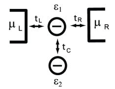
Figure 1: The T-shaped double-dot system. The upper dot, dot 1, is connected to the external leads by the tunneling matrix elements $t_{\rm L}$ and $t_{\rm R}$; dot 2 is connected, by the tunneling matrix element $t_{\rm C}$, solely to dot 1. Both dots are represented by a single energy level each, $\varepsilon_{1}$ and $\varepsilon_{2}$.

The dotted line in Fig. 2 is the differential conductance computed from Eq. (1) for a symmetric DQD, $\varepsilon=\varepsilon_{1}=\varepsilon_{2}$ and $\alpha=1$. It has a double-peak structure with a dip in-between. The two peaks reflect resonant tunneling through the bonding and anti-bonding orbital states of the quantum dots, yielding $dI/dV=2e^{2}/h$. At the midpoint between the peaks the differential conductance vanishes due to fully destructive interference. This structure resembles a Fano resonance in a special case; fano indeed the conductance may be fitted to the Fano line shape, $(q+E)^{2}/(E^{2}+\gamma^{2})$, where in our case, $E=\tilde{E}_{2}$, $\tilde{E}_{1}=0$, $q=0$, and $\gamma=2|\tilde{t}_{\rm C}|^{2}$.

In the presence of e-ph interactions, this double-peak structure is modified significantly, as exemplified by the full curve in Fig. 2. Of particular interest is the effect of those interactions on the destructive interference leading to the dip: we find that only the e-ph interaction on dot 2 is responsible for the ascent of the dip. Moreover, we argue that the dependence of this ascent on the bias voltage reflects the effective coupling of the e-ph interaction on dot 2, and hence may serve for phonon spectroscopy. The effect of the e-ph interaction taking place on dot 1, together with the one on dot 2, is to decrease the peaks’ height as compared to the zero-interaction case.

Below, we study separately the case of e-ph interactions with acoustic phonons, and with optical ones. In semiconductor quantum dots, the electrons interact with the bulk phonons of the semiconductor base. Then, the electronic interaction with acoustic phonons plays a major role at low temperatures since the energies of the optical phonons are much larger ($\sim 36meV$ for GaAs) than those of the acoustic phonons. bruus ; keil In the case of e-ph interaction with acoustic phonons the density of available states is continuous, and indeed we find that the dip in the conductance rises up gradually as the bias voltage increases.

The interaction of transport electrons with optical modes is considered to be dominant in molecular junctions park ; smit ; zhitenev ; tal ; leroy which do not lie on a substrate. Several theoretical works studying e-ph interactions in molecular junctions have employed as a model of the molecular bridge a single-level quantum dot coupled to optical vibrations, calculating the differential conductance galperin ; mitra ; egger ; ora ; ora2 ; hod ; koch ; ryndyk ; koch2 and the shot noise. haupt ; avriller ; schmidt We find that the interaction with optical phonons affects the dip once the bias voltage matches the vibrational energy on dot 2, but not on dot 1. A delicate issue is the question of the population of the vibrational states. ora2 When the e-ph interaction is with the acoustic phonons of the substrate, one may assume that those are given by the thermal-equilibrium distribution. This assumption does not necessarily hold for interactions on molecular bridges, where the population of the vibrational modes may be determined mainly by the transport electrons. Here we will assume that the molecular vibrations are thermalized by a coupling with the phonon bath of the surrounding.

The organization of the paper is as follows. We begin in Sec. II by describing our model and presenting the expression for the differential conductance through the T-shape system. The technical details of the calculation are described in the Appendix, in particular the treatment of the electron-phonon interaction in the self-consistent Born approximation.ueda2 ; ueda3 For clarity, we confine ourselves to the case of zero temperature. Then, the transport electrons can only emit phonons once the bias voltage exceeds the phonon energy. Section III is devoted to the analysis of our results. First, we discuss the dephasing-free phonon emission. We show that the conductance dip is not affected by phonon emission from dot 1. Second, we examine the conductance dip as a function of the bias voltage $V$. We show that the amount of decrease in the dip as the bias voltage is increased follows the product of the phonons’ density of states and the coupling strength of e-ph interaction. We conclude by a summary/discussion section.

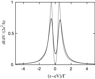
Figure 2: The differential conductance $dI/dV$ of a symmetric ($\varepsilon=\varepsilon_{1}=\varepsilon_{2}$, $\alpha=1$) DQD structure as a function of the gate voltage $\varepsilon$. In the absence of the e-ph interaction, the conductance follows the dotted curve. The solid line is the differential conductance when the transport electrons are coupled to acoustic phonons on both dots. Here $t_{\rm C}=0.5\Gamma$.

II The model and the calculation method

II.1 The model

Our model system is depicted in Fig. 1, and is described by the Hamiltonian

$$H=H_{\rm el}+H_{\rm{e-ph}}+H_{\rm ph}\ .$$ (2)

Omitting the spin indices, the Hamiltonian of the electrons is

$$H_{\rm{el}} =H_{\rm{L}}+H_{\rm{R}}+H_{\rm{T}}+H_{\rm{D}}.$$ (3)

It consists of the leads’ Hamiltonian

$$H_{\rm{L(R)}} =\sum_{k}\varepsilon_{k}c^{\dagger}_{{\rm{L(R)}}k}c_{{\rm{L(R)}}k},$$ (4)

the DQD Hamiltonian

$$H_{\rm{D}} =\varepsilon_{1}d_{1}^{\dagger}d_{1}+\varepsilon_{2}d_{2}^{\dagger}d_{2},$$ (5)

and the tunneling Hamiltonian

$$H_{\rm{T}} =\sum_{k}(t_{\rm{L}}c^{\dagger}_{{\rm{L}}k}d_{1}+{\rm H.c.})+\sum_{k}(t_{\rm{R}}c^{\dagger}_{{\rm{R}}k}d_{1}+{\rm H.c.})$$

$$\quad+t_{\rm C}(d_{1}^{\dagger}d_{2}+\rm{H.c.}).$$ (6)

Here, $c^{\dagger}_{{\rm{L(R)}}k}$ and $c_{{\rm{L(R)}}k}$ denote the creation and annihilation operators of an electron of momentum $k$ in lead L (R), respectively. We assume a single energy level $\varepsilon_{1}$ in dot 1 ($\varepsilon_{2}$ in dot 2), with the creation and annihilation operators on that level being $d_{1}^{\dagger}$, $d_{1}$ ($d_{2}^{\dagger}$, $d_{2}$). Electronic correlations are not included in our analysis. The broadening of the resonant level on dot 1, $\Gamma=\Gamma_{\rm L}+\Gamma_{\rm R}$, is given by $\Gamma_{\rm L(R)}=2\pi\nu t^{2}_{\rm L(R)}$, where $\nu$ is the density of states of the electrons in the leads, and $t_{\rm L}$ ($t_{\rm R})$ is the tunneling matrix element connecting the dots to the left (right) lead.

We consider e-ph interactions which are confined to the DQD. In the case of acoustic phonons, the interaction Hamiltonian reads

$$H_{\rm{e-ph}} =\sum_{\bm{q}}M_{\bm{q},1}(a_{\bm{q}}+a^{\dagger}_{-\bm{q}})d_{1}^{\dagger}d_{1}$$

$$+\sum_{\bm{q}}M_{\bm{q},2}(a_{\bm{q}}+a^{\dagger}_{-\bm{q}})d_{2}^{\dagger}d_{2},$$ (7)

with the acoustic phonon Hamiltonian being

$$H_{\rm ph}= \sum_{\bm{q}}\omega_{\bm{q}}a^{\dagger}_{\bm{q}}a_{\bm{q}}.$$ (8)

Here, $a_{\bm{q}}^{\dagger}$ and $a_{\bm{q}}$ are the creation and annihilation operators of phonons with momentum $\bm{q}$. We disregard the possibility of nonlocal e-ph interactions, $(a_{\bm{q}}+a^{\dagger}_{-\bm{q}})d^{\dagger}_{2}d_{1}$, assuming that the overlap between the wave functions of dot 1, $|d_{1}\rangle$, and dot 2, $|d_{2}\rangle$, is small. The dispersion relation of the acoustic phonons is taken to be linear,

$$\omega_{\bm{q}}=c_{\rm S}|{\bm{q}}|$$ (9)

with the sound velocity $c_{\rm S}$. When the e-ph interaction with acoustic phonons originates from the piezoelectric coupling, the matrix element of the coupling with the electron is keil ; bruus

$$M_{{\bm{q}},i}=\lambda_{\bm{q}}\langle d_{i}|e^{i{\bm{q}}\cdot{\bm{r}}}|d_{i}\rangle,$$ (10)

with

$$|\lambda_{\bm{q}}|^{2}=g\frac{\pi^{2}c_{\rm S}^{2}}{|\bm{q}|}.$$ (11)

For example, in GaAs $g=0.1$. Because of the oscillating factor $e^{i{\bm{q}}\cdot{\bm{r}}}$, the e-ph interaction decreases once the wavelength of the phonons is smaller than the size of the dot $L_{i}$ ($i=1,2$). For this reason one may choose

$$|M_{{\bm{q}},i}|^{2}=\frac{\sqrt{2}}{\pi^{1/2}L^{2}_{i}}\frac{|\lambda_{\bm{q}}|^{2}}{|{\bm{q}}|^{2}+(1/L_{i})^{2}}.$$ (12)

(The effect of the mixed product $M_{{\bm{q}},i}M^{\ast}_{{\bm{q}},j}$ for $i\neq j$ is negligible, because the phase-differnece between the two matrix elements that depends on the inter-dot distance diminishes its contribution.)

An ubiquitous model to describe the interaction with optical phonons is the Fröhlich Hamiltonian,mahan treating the quantum dots as Einstein oscillators of frequency $\omega_{i}$, $i=1,2$. In that case the electron-phonon Hamiltonian reads

$$H_{\rm{e-ph}} =\zeta_{1}(a_{1}+a^{\dagger}_{1})d_{1}^{\dagger}d_{1}+\zeta_{2}(a_{2}+a^{\dagger}_{2})d_{2}^{\dagger}d_{2},$$ (13)

and the phonon Hamiltonian is

$$H_{\rm ph} =\omega_{1}a^{\dagger}_{1}a_{1}+\omega_{2}a^{\dagger}_{2}a_{2},$$ (14)

where $a_{i}$ and $a_{i}^{\dagger}$ are the creation and the annihilation operators of phonons on dot $i$ and $\zeta_{i}$ is the coupling strength of the optical e-ph interaction.

Using the Keldysh formalism,keldysh ; caroli ; jauho the current can be expressed in terms of the Fourier transform of the retarded Green function of dot 1, $G^{r}_{11}(t-t^{\prime})=-i\theta(t-t^{\prime})\langle\{d_{1}(t),d^{\dagger}_{1}(t^{\prime})\}\rangle$,

$$I=\frac{2e}{h}\int d\omega\Bigl{(}-\frac{\alpha}{2}\Gamma\Bigr{)}[f_{\rm L}(\omega)-f_{\rm R}(\omega)]{\rm Im}G^{r}_{\rm{11}}(\omega),$$ (15)

see the Appendix for details. Here, $f_{\rm L(R)}(\omega)=(\exp[\beta(\omega-\mu_{\rm L(R)})]+1)^{-1}$ is the Fermi distribution function in lead L (R). In this paper we study the differential conductance, given by

$$\frac{dI}{dV}=-\frac{2e^{2}}{h}\frac{\alpha}{2}\Gamma\bigl{[}{\rm Im}G^{r}_{11}(eV)+\int^{eV}_{0}d\omega{\rm Im}\frac{dG^{r}_{11}(\omega)}{d(eV)}\bigr{]},$$ (16)

where the explicit form of $G^{r}_{11}(\omega)$, in terms of the self-energies, is (see the Appendix)

$$G^{r}_{11}(\omega)=\frac{\omega-\varepsilon_{2}}{(\omega-\varepsilon_{1})(\omega-\varepsilon_{2})+\frac{i}{2}\Gamma(\omega-\varepsilon_{2})-|t_{\rm C}|^{2}-(\omega-\varepsilon_{2})\Sigma^{r}_{11}(\omega)-\frac{|t_{\rm C}|^{2}}{\omega-\varepsilon_{2}}\Sigma^{r}_{22}(\omega)}.$$ (17)

III Results

We begin with results pertaining to the case in which the electrons are coupled to acoustic phonons, see Eq. (7). In Fig. 3 we plot the variation of the differential conductance of a completely symmetric DQD with the gate voltage, scaling all energies by $\Gamma$, the level broadening on dot 1. We present separately results for the case where the e-ph interaction takes place on dot 1 alone [panel (a)] or on dot 2 alone [panel (b)]. Both panels show also the differential conductance obtained in the absence of the coupling with the acoustic phonons. (The parameters chosen are given in the caption of Fig. 3.) As is seen from Fig. 3, while phonon emission from dot 1 does not affect the dip in the differential conductance, it has a detrimental effect on $dI/dV$ when it occurs on dot 2. The destructive interference leading to the dip in the differential conductance is severely harmed by the e-ph interaction on dot 2.

To explain this observation, we treat the e-ph interaction to second-order in perturbation theory (note, however, that the plots in Fig. 3 were computed in the self-consistent Born approximation). The dip in $dI/dV$, Eq. (16), occurs at $\varepsilon=eV$. Then, the first term there vanishes [since at zero temperature ${\rm Im}G^{r}_{11}(eV)=0$] while the second term yields

$$\frac{dI}{dV}=\frac{2e^{2}}{h}\frac{\alpha\Gamma}{2}{\rm Im}\Bigl{(}\int^{eV}_{0}d\omega\Bigr{[}(\omega-eV)^{2}+\frac{i}{2}\Gamma(\omega-eV)-|t_{\rm C}|^{2}-(\omega-eV)\Sigma^{r}_{11}(\omega)-\frac{|t_{\rm C}|^{2}}{\omega-eV}\Sigma^{r}_{22}(\omega)\Bigr{]}^{-2}$$

$$\times\Bigl{[}(\omega-eV)^{2}\frac{d\Sigma^{r}_{11}(\omega)}{deV}+|t_{\rm C}|^{2}\frac{d\Sigma^{r}_{22}(\omega)}{deV}\Bigr{]}\Bigr{)}.$$ (18)

Calculating the self-energies appearing in this expression in second-order perturbation theory we find

$$\Sigma^{r(2)}_{11}(\omega) =\sum_{\bm{q}}|M_{{\bm{q}},1}|^{2}\int\frac{d\omega^{\prime}}{2\pi}|G^{r(0)}_{11}(\omega-\omega^{\prime})|^{2}$$

$$\times\Bigl{\{}\frac{\Gamma_{\rm L}f_{\rm L}(\omega-\omega^{\prime})+\Gamma_{\rm R}f_{\rm R}(\omega-\omega^{\prime})}{\omega^{\prime}-\omega_{\bm{q}}+i0^{+}}+\frac{\Gamma_{\rm L}[1-f_{\rm L}(\omega-\omega^{\prime})]+\Gamma_{\rm R}[1-f_{\rm R}(\omega-\omega^{\prime})]}{\omega^{\prime}+\omega_{\bm{q}}+i0^{+}}\Bigr{\}},$$ (19)

and

$$\Sigma^{r(2)}_{22}(\omega) =\sum_{\bm{q}}|M_{{\bm{q}},2}|^{2}\int\frac{d\omega^{\prime}}{2\pi}|G^{r(0)}_{12}(\omega-\omega^{\prime})|^{2}$$

$$\times\Bigl{\{}\frac{\Gamma_{\rm L}f_{\rm L}(\omega-\omega^{\prime})+\Gamma_{\rm R}f_{\rm R}(\omega-\omega^{\prime})}{\omega^{\prime}-\omega_{\bm{q}}+i0^{+}}+\frac{\Gamma_{\rm L}[1-f_{\rm L}(\omega-\omega^{\prime})]+\Gamma_{\rm R}[1-f_{\rm R}(\omega-\omega^{\prime})]}{\omega^{\prime}+\omega_{\bm{q}}+i0^{+}}\Bigr{\}}.$$ (20)

A straightforward calculation shows that $d\Sigma^{r(2)}_{11}(\omega)/d(eV)$ at $\epsilon=eV$ vanishes [this follows from Eq. (17)]. Hence, when the e-ph interaction on dot 2 vanishes, so does the differential conductance at the mid-point. On the other hand,

$$\frac{\Sigma^{r(2)}_{22}(\omega)}{deV}= -\sum_{\bm{q}}\frac{|M_{{\bm{q}},2}|^{2}}{2\pi}\frac{\Gamma_{\rm L}}{|t_{\rm C}|^{2}}\Bigl{(}\frac{1}{\omega-\omega_{\bm{q}}-eV+i0^{+}}-\frac{1}{\omega+\omega_{\bm{q}}-eV+i0^{+}}\Bigr{)}$$

$$=\frac{g}{2(2\pi)^{1/2}}\frac{\Gamma_{\rm L}}{|t_{\rm C}|^{2}}\bigl{(}\frac{c_{\rm S}}{L_{2}}\bigr{)}^{2}\frac{\omega-eV}{(\omega-eV)^{2}+(c_{\rm S}/L_{2})^{2}},$$ (21)

yielding that when phonon emission takes place on dot 2 the dip in the differential conductance is modified.

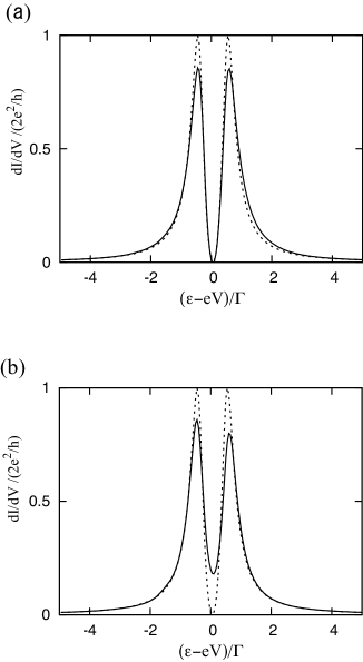
Figure 3: The differential conductance $dI/dV$ (solid lines) as a function of the gate voltage $\varepsilon$ of a symmetric DQD ($\varepsilon=\varepsilon_{1}=\varepsilon_{2}$, $\alpha=1$), for e-ph coupling with acoustic phonons. The bias voltage is $eV=2\Gamma$ and $t_{\rm C}=0.5\Gamma$ ($\Gamma$ is the level broadening on dot 1). Panel (a): the e-ph interaction is on dot 1 alone; panel (b): the e-ph interaction is on dot 2 alone. The dotted curves are the differential conductance when the e-ph interactions are absent.

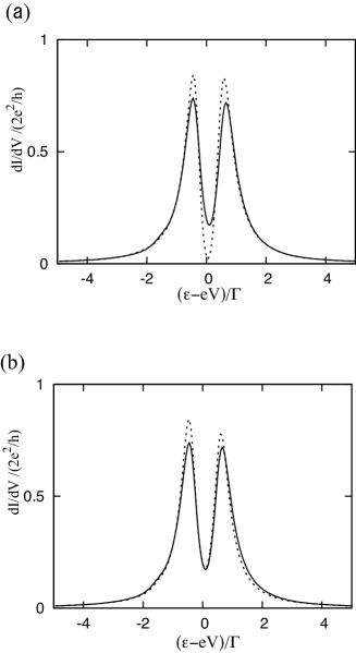
Figure 4: The differential conductance $dI/dV$ as a function of the gate voltage $\varepsilon$ of a symmetric DQD ($\varepsilon=\varepsilon_{1}=\varepsilon_{2}$, $\alpha=1$), for e-ph coupling with acoustic phonons. The bias voltage is $eV=2\Gamma$ and $t_{\rm C}=0.5\Gamma$ ($\Gamma$ is the level broadening on dot 1). Panel (a): changing the size of dot 2. The solid line is the differential conductance when both dot sizes are equal, $L_{1}=L_{2}=c_{\rm S}/{(2.0\Gamma})$ and the dotted line is for the case $L_{1}=c_{\rm S}/{(2.0\Gamma})$ and $L_{2}=c_{\rm S}/{(0.5\Gamma})$. Panel (b): changing the size of dot 1. The solid line is the differential conductance when both dot sizes are equal, $L_{1}=L_{2}=c_{\rm S}/({2.0\Gamma})$ and the dotted line is f or the case $L_{1}=c_{\rm S}/{(0.5\Gamma})$ and $L_{2}=c_{\rm S}/{(2.0\Gamma})$.

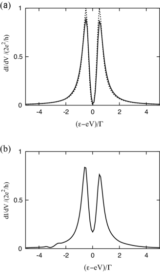
Figure 5: The differential conductance $dI/dV$ as a function of the gate voltage $\varepsilon$ of a symmetric DQD ($\varepsilon=\varepsilon_{1}=\varepsilon_{2}$, $\alpha=1$), for e-ph coupling with optical phonons. Here $t_{\rm C}=0.5\Gamma$ ($\Gamma$ is the level broadening on dot 1), and the strengths of e-ph coupling on the dots are $\zeta_{1}=\zeta_{2}=0.3\Gamma$. $\delta$ introduced in Eqs. (37) and (38) is $\delta=0.5\Gamma$. Panel (a): the phonon energy in dot 1 (dot 2) is $\omega_{1}=\Gamma$ ($\omega_{2}=3\Gamma$), and the bias voltage is $eV=\Gamma$. The dotted line indicates the conductance in the absence of e-ph interaction. Panel (b): the same as in (a) with $eV=3\Gamma$.

Since the e-ph interaction on dot 1 does not harm the interference around $\epsilon=eV$, one may say that it does not cause dephasing. One may monitor this (zero-temperature) dephasing-free phonon emission by varying the size of the DQD. As is mentioned above [see Eq. (12)], the efficacy of the e-ph interaction with acoustic phonons depends on the dot size: it decreases as the dot size increases. The effect of the two dots’ sizes on the differential conductance is investigated in Fig. 4. In both panels, the solid curves pertain to the case of equal-size dots. The dotted curve in panel (a) shows the modification in the differential conductance brought about by increasing the size of dot 2 (thus making the phonon emission there less efficient). It is clearly seen that the decrease in $dI/dV$ towards the dip is severely disturbed. On the other hand, when the size of dot 1 is increased [panel (b)] the differential conductance is almost unchanged.

Next we consider the differential conductance in the case where the electrons are coupled to optical phonons. The main difference between this interaction and the coupling with acoustic phonons discussed above, is that now the transport electrons can emit real phonons and change their energies only when the bias voltage exceeds the phonon frequency (at zero temperature). This is portrayed in Fig. 5. Switching-on the coupling to optical phonons when the vibration frequency on dot 2 is larger than the bias voltage almost makes no difference in the shape of the differential conductance [see panel (a) of Fig. 5]. The modifications in the peaks’ heights are due to elastic processes taking place on both dots. On the other hand, when the bias voltage is large enough (as compared to the vibration frequency on dot 2), there is a significant effect on the dip in $dI/dV$, see panel (b) of Fig. 5.

Finally we study the possibility to use the dephasing effect of the e-ph interactions on dot 2 for phonon spectroscopy. Figure 6 depicts the dependence of the conductance at the dip on the bias voltage for coupling with acoustic phonons [panel (a)] and optical phonons [panel (b)]. The coupling of the electrons to acoustic phonons is characterized by the spectral function obtained from the product of their density of states and the (acoustic) e-ph matrix element squared,

$$\chi(\omega) =\sum_{\bm{q}}|M_{\bm{q},2}|^{2}\delta(\omega-\omega_{\bm{q}})$$ (22)

$$=\frac{g}{(2\pi)^{1/2}}\bigl{(}\frac{c_{\rm S}}{L_{2}}\bigr{)}^{2}\frac{\omega}{\omega^{2}+(c_{\rm S}/L_{2})^{2}}.$$ (23)

Only the spectral function on dot 2 is presented, since (as was elaborated upon above) the conductance dip is affected by the e-ph interaction on that dot. The function $\chi(\omega)$ is shown by the dotted curve of Fig. 6. Although it does not coincide with the conductance curve it does follow it, in particular at higher values of the voltage.

Panel (b) of Fig. 6 shows the value of the conductance dip (as a function of the bias voltage) in the case where the electrons are coupled to optical phonons. The prominent feature here is the peak obtained when the bias voltage matches the vibration frequency on dot 2. The decrease in the conductance dip becomes more pronounced as the tunnel coupling between the two dots, $t_{\rm C}$, is decreased. This is because when this coupling is strong, separate effects of the dots on the conductance is more blurred. On the other hand, a smaller value of this coupling enables the manifestation of the e-ph interaction on dot 2 to become more distinguished. We do not plot the spectral function corresponding to the case of optical phonons since our calculation does not take into consideration the origin of the life time of these phonons. The broadening $\delta$ introduced in Eqs. (37) and (38) is a free parameter, that in fact can be extracted by fitting the curves in Fig. 6 (b) to the experimental data.

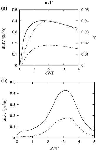
Figure 6: The differential conductance $dI/dV$ as a function of the bias voltage $V$ for a symmetric DQD ($\varepsilon=\varepsilon_{1}=\varepsilon_{2}$, $\alpha=1$), at the conductance dip ($\varepsilon-eV=0$). The tunnel coupling between the dots is $t_{\rm C}=0.3\Gamma$ (solid lines) and $t_{\rm C}=0.5\Gamma$ (dashed lines). Panel (a): coupling with acoustic phonons; the dotted line is $\chi(\omega)$ [Eq. (23)] as a function of $\omega$ (marked on the right-side vertical axis). Panel (b): coupling with optical phonons. The vibration energy in dot 1 is $\omega_{1}=\Gamma$ and on dot 2 is $\omega_{2}=3\Gamma$.

IV Discussion

In summary, we have studied the effect of electron-phonon interactions in a T-shaped DQD, employing the self-consistent Born approximation. The differential conductance of this device is characterized by the appearance of a double-peak structure due to interference. The dip in-between the two peaks is quite sensitive to the dephasing effect of phonon emission. We find that while phonon emission from dot 1 does not affect the conductance dip, phonon emission from dot 2 leads to its ascent. Therefore, the electron-phonon interaction on dot 2, in particular the effective e-ph coupling given by the product of the phonons’ density of states and the e-ph interaction, can be probed electrically, by monitoring the variation of the conductance dip.

The conductance dip always appears at $\varepsilon_{2}=eV$, even when the DQD is asymmetric (for example, $\varepsilon_{1}\neq\varepsilon_{2}$). Since the behavior of the self energy, which is responsible for the appearance of the dip, remains the same also in this case, our conclusions should hold for the asymmetric double-quantum-dot system. On the other hand, we expect that a finite temperature will smear the conductance dip (even in the absence of the electron-phonon interactions). When the temperature differs from zero, the behavior of the self energy is slightly (at low temperature) modified, and the distinction between the effects of the e-ph interactions on dot 1 and those on dot 2 is less clear. A finite temperature will also facilitate phonon absorption processes. However, these alone are not expected to modify our main results considerably. One may hope though, that phonon spectroscopy via the monitoring of the conductance dip is still possible at low enough temperatures. This in particular is so since we propose to monitor the differential conductance at finite bias voltages.

An interesting point is the experimental possibility to have the electron-phonon interaction taking place mainly on one of the dots forming the DQD system. A phonon bath may be realized by an electronically insulating hard substrate. It is harder to imagine how a quantum dot can be effectively detached from a phonon bath and become “floating”; this seems to be more realistic in the case of a molecular junction, for which, under these circumstances, the relevant vibrational modes are optical. Then, a sufficiently high phonon frequency (higher than the bias voltage required for the dip) will satisfy the above requirement.

Appendix A Details of the calculation

Our calculation requires all four Keldysh Green functions keldysh ; caroli ; jauho belonging to the DQD: the time-ordered one

$$G^{t}_{ij}(t-t^{\prime}) =-i\langle\mathcal{T}d_{i}(t)d^{\dagger}_{j}(t^{\prime})\rangle,$$ (24)

the anti time-ordered one,

$$G^{\tilde{t}}_{ij}(t-t^{\prime}) =-i\langle\tilde{\mathcal{T}}d_{i}(t)d_{j}^{\dagger}(t^{\prime})\rangle,$$ (25)

with $\mathcal{T}$ ($\tilde{\mathcal{T}}$) being the time-ordering (anti time-ordering) operator, and the lesser and greater Green functions,

$$G^{<}_{ij}(t-t^{\prime}) =i\langle d_{j}^{\dagger}(t^{\prime})d_{i}(t)\rangle,$$

$$G^{>}_{ij}(t-t^{\prime}) =-i\langle d_{i}(t)d_{j}^{\dagger}(t^{\prime})\rangle.$$ (26)

Here $i$ and $j$ take the values 1 and 2.

It is convenient to present the Fourier transforms of these Green functions in a matrix form

$$\bm{G}^{\gamma}(\omega)=\begin{pmatrix}G^{\gamma}_{11}(\omega)&G^{\gamma}_{12}(\omega)\\ G^{\gamma}_{21}(\omega)&G^{\gamma}_{22}(\omega)\end{pmatrix}$$ (27)

where $\gamma=t$, $\tilde{t}$, $<$, or $>$. The retarded and advanced Green functions follow from these functions,

$$\bm{G}^{r}(\omega)=\bm{G}^{t}(\omega)-\bm{G}^{<}(\omega).$$ (28)

All the necessary Green functions are obtained from the corresponding Dyson equations, in which there appears the self-energy due to the e-ph interaction, $\Sigma$,

$$\bm{G}^{r}(\omega) =\bm{G}^{r(0)}+\bm{G}^{r(0)}(\omega)\bm{\Sigma}^{r}(\omega)\bm{G}^{r}(\omega),$$ (29)

and the lesser Green function of the DQD

$$\bm{G}^{<}(\omega)=\bm{G}^{r}(\omega)\bm{\Sigma}^{<}(\omega)\bm{G}^{a}(\omega)$$

$$+[1+\bm{G}^{r}(\omega)\bm{\Sigma}^{r}(\omega)]\bm{G}^{<(0)}(\omega)[1+\bm{\Sigma}^{a}(\omega)\bm{G}^{a}(\omega)],$$ (30)

where $\bm{G}^{(0)}$ is the Green function in the absence of the coupling to the phonons.

We treat the e-ph interactions in the self-consistent Born approximation. ueda2 ; ueda3 Since we focus on the effect of the inelastic electron-phonon processes, we discard the Hartree term. When the transport electrons are coupled to acoustic phonons, the required self-energies are

$$\Sigma^{t}_{ii}=\frac{i}{2\pi}\sum_{\bm{q}}|M_{\bm{q},i}|^{2}\int d\omega^{\prime}G_{ii}^{t}(\omega-\omega^{\prime})D^{t}(\bm{q},\omega^{\prime}),$$ (31)

and

$$\Sigma^{<}_{ii}=\frac{i}{2\pi}\sum_{\bm{q}}|M_{\bm{q},i}|^{2}\int d\omega^{\prime}G_{ii}^{<}(\omega-\omega^{\prime})D^{<}(\bm{q},\omega^{\prime}).$$ (32)

Here $D$ denotes the Fourier transform of the zero-order (i.e., in the absence of the coupling to the electrons) phonon Green functions,

$$D^{t}({\bm{q}},\omega) =-2\pi i[N_{\bm{q}}\delta(\omega+\omega_{\bm{q}})+N_{\bm{q}}\delta(\omega-\omega_{\bm{q}})]$$

$$\quad+\frac{1}{\omega-\omega_{\bm{q}}+i0^{+}}-\frac{1}{\omega+\omega_{\bm{q}}-i0^{+}},$$ (33)

and

$$D^{<}({\bm{q}},\omega) =-2\pi i[(N_{\bm{q}}+1)\delta(\omega+\omega_{\bm{q}})$$

$$+N_{\bm{q}}\delta(\omega-\omega_{\bm{q}})],$$ (34)

where $N_{\bm{q}}$ is the phonon population of mode ${\bm{q}}$. It is implicitly assumed that the vibrational modes are equilibrated by the coupling to another heat bath, such that their population is given by Bose-Einstein distribution function, $1/[\exp(\beta\omega_{\bm{q}})-1]$. Then, $N_{\rm q}=0$ at zero temperature. The self-energies $\Sigma^{r}_{ii}(\omega)$ and $\Sigma^{<}_{ii}$ are determined by solving Eqs. (31) and (32) self-consistently.

When the electrons are coupled to optical phonons, the self-energies are

$$\Sigma^{t}_{ii}=\frac{i}{2\pi}\zeta_{i}^{2}\int d\omega^{\prime}G_{ii}^{t}(\omega-\omega^{\prime})D^{t}_{i}(\bm{q},\omega^{\prime}),$$ (35)

and

$$\Sigma^{<}_{ii}=\frac{i}{2\pi}\zeta_{i}^{2}\int d\omega^{\prime}G_{ii}^{<}(\omega-\omega^{\prime})D^{<}_{i}(\bm{q},\omega^{\prime}),$$ (36)

where the Fourier transforms of phonon Green functions at zero temperature are

$$D^{t}_{i}(\omega)=\frac{1}{\omega-\omega_{i}+i\delta}-\frac{1}{\omega+\omega_{i}-i\delta},$$ (37)

and

$$D^{<}_{i}(\omega)=\frac{1}{\omega+\omega_{i}+i\delta}-\frac{1}{\omega+\omega_{i}-i\delta}.$$ (38)

Here $\delta$ is relaxation rate of the Einstein phonon mode due to the coupling with the surrounding bulk phonons. As in the acoustic-phonon case, $\Sigma^{r}_{ii}(\omega)$ and $\Sigma^{<}_{ii}$ are determined by solving Eqs. (35) and (36) self-consistently.

The Green functions of the DQD, in particular $G^{r}_{11}$, determine the expression for the current. The operator of the current between the left lead and the quantum dots is given by the time derivative of the electron number operator in that lead, $N_{\rm{L}}=\sum_{k}c^{\dagger}_{{\rm L}k}c_{{\rm L}k}$,

$$I_{\rm{L}}=-2e\langle{\dot{N}_{\rm{L}}}\rangle =-2ie\langle[H,N_{\rm{L}}]\rangle=4e{\rm Re}\sum_{k}t_{\rm{L}}G^{<}_{{\rm 1,L}k}(t,t)$$

$$=\frac{4e}{h}{\rm Re}\int d\omega t_{\rm{L}}\sum_{k}G^{<}_{{\rm 1,L}k}(\omega)\ ,$$ (39)

adding a factor of 2 for the spin components. Here $G^{<}_{{\rm 1,L}k}(t-t^{\prime})=i\langle c^{\dagger}_{{\rm L}k}(t^{\prime})d_{1}(t)\rangle$ is the lesser Green function and $G^{<}_{{\rm 1,L}k}(\omega)$ is its Fourier transform. The current from lead R to the quantum dots, $I_{\rm R}$, is obtained in the same way.

Using the equation-of-motion method jauho the current from lead L (R) is rewritten as

$$I_{\rm L(R)}= \frac{4e}{h}\int d\omega\biggl{[}-\frac{\Gamma_{\rm L(R)}}{2}{\rm Im}G^{<}_{\rm{11}}(\omega)$$

$$-\Gamma_{\rm L(R)}f_{\rm L}(\omega){\rm Im}G^{r}_{\rm{11}}(\omega)\biggr{]},$$ (40)

where $G^{r}$ denotes the retarded Green function. The net current through the DQD system is hence

$$I =\frac{1}{2}\Bigl{(}I_{\rm L}-I_{\rm R}\Bigr{)}$$

$$=\frac{4e}{h}\int d\omega\biggl{\{}-\frac{1}{4}\Bigl{(}\Gamma_{\rm L}-\Gamma_{\rm R}\Bigr{)}{\rm Im}G^{<}_{\rm{11}}(\omega)$$

$$-\frac{1}{2}\Bigl{(}\Gamma_{\rm L}f_{\rm L}(\omega)-\Gamma_{\rm R}f_{\rm R}(\omega)\Bigr{)}{\rm Im}G^{r}_{\rm{11}}(\omega)\biggr{\}}.$$ (41)

Using the relation $I_{\rm L}+I_{\rm R}=0$ which follows by charge conservation, and assuming that the widths $\Gamma_{\rm L}$ and $\Gamma_{\rm R}$ do not vary significantly with energy, we can express the lesser Green function in terms of the retarded one,

$${\rm Im}G^{<}_{11}(\omega)=-\frac{2[\Gamma_{\rm L}f_{\rm L}(\omega)+\Gamma_{\rm R}f_{\rm R}(\omega)]}{\Gamma_{\rm L}+\Gamma_{\rm R}}{\rm Im}G^{r}_{\rm{11}}(\omega).$$ (42)

Inserting Eq. (42) in Eq. (41) leads to Eq. (15).

References

- (1) A. Yacoby, M. Heiblum, D. Mahalu, and H. Shtrikman, Phys. Rev. Lett. 74, 4047 (1995).
- (2) R. Schuster, E. Buks, M. Heiblum, D. Mahalu, V. Umansky, and H. Shtrikman, Nature (London) 385, 417 (1997).
- (3) K. Kobayashi, H. Aikawa, S. Katsumoto, and Y. Iye, Phys. Rev. Lett. 88, 256806 (2002); Phys. Rev. B 68, 235304 (2003).
- (4) Y. Aharonov and D. Bohm, Phys. Rev. 115, 485 (1959).
- (5) H. Akera, Phys. Rev. B 47, 6835 (1993).
- (6) J. König and Y. Gefen, Phys. Rev. Lett. 86, 3855 (2001); Phys. Rev. B 65, 045316 (2002).
- (7) F. Marquardt and C. Bruder, Phys. Rev. B 68, 195305 (2003).
- (8) A. Ueda, I. Baba, K. Suzuki, and M. Eto, J. Phys. Soc. Jpn. Suppl. A 73, 157 (2003).
- (9) A. Ueda and M. Eto, Phys. Rev. B 73, 235353 (2006).
- (10) A. Ueda and M. Eto, N. J. Phys. 9, 119 (2007).
- (11) U. Fano, Phys. Rev. 124, 1866 (1961).
- (12) J. Koch and F. von Oppen, Phys. Rev. Lett. 94, 206804 (2005).
- (13) O. Entin-Wohlman, Y. Imry, and A. Aharony, Phys. Rev. B 80, 035417 (2009).
- (14) A. Stern, Y. Aharonov, and Y. Imry, Phys. Rev. A 41, 3436 (1990).
- (15) H. Bruus, K. Flensberg, and H. Smith, Phys. Rev. B 48, 11144 (1993).
- (16) M. Keil and H. Schoeller, Phys. Rev. B 66, 155314 (2002).
- (17) H. Park, J. Park, A. K. L. Lim, E. H. Anderson, A. P. Alivisatos, and P. L. MacEuen, Nature (London), 407, 57 (2000).
- (18) R. Smit, Y. Noat, C. Uniteiedt, N. D. Lang, M. C. van Hemert, and J. M. van Ruitenbeek, Nature (London) 419, 906 (2002).
- (19) N. B. Zhitenev, H. Meng, and Z. Bao, Phys. Rev. Lett. 88, 226801 (2002).
- (20) B. J. LeRoy, S. G. Lemay, J. Kong, and C. Dekker, Nature (London) 432, 371 (2004).
- (21) O. Tal, M. Krieger, B. Leerink, and J. M. van Ruitenbeek, Phys. Rev. Lett. 100, 196804 (2008).
- (22) M. Galperin, M. A. Ratner, and A. Nitzan, Nano Lett. 4, 1605 (2004). J. Phys: Condens. Matter, 19, 103201 (2007).
- (23) A. Mitra, I. Aleiner, and A. J. Millis, Phys. Rev. B 69, 245302 (2004); Phys. Rev. Lett. 94, 076404 (2005).
- (24) D. A. Ryndyk and J. Keller, Phys. Rev. B 71, 073305 (2005).
- (25) J. Koch, M. Semmelhack, F. von Oppen, and A. Nitzan, Phys. Rev. B 73, 155306 (2006).
- (26) O. Hod, R. Baer, and E. Rabani, Phys. Rev. Lett. 97, 266803 (2006); J. Phys: Condens. Matter, 20, 383201 (2008).
- (27) R. Egger and A. O. Gogolin, Phys. Rev. B 77, 113405 (2008).
- (28) O. Entin-Wohlman, Y. Imry, and A. Aharony, Phys. Rev. B 81, 113408 (2010).
- (29) T. L. Schmidt and A. Komnik, Phys. Rev. B 80, 041307(R) (2009).
- (30) R. Avriller and A. Levy Yeyati, Phys. Rev. B 80, 041309(R) (2009).
- (31) F. Haupt, T. Novotny, and W. Belzig, Phys. Rev. Lett. 103, 136601 (2009).
- (32) G. D. Mahan, Many-Particle Physics (Plenum Press, New York, 1990).
- (33) L. V. Keldysh, Zh. Ekps. Teor. Fiz. 47, 1515 (1964) [Sov. Phys. JETP 20,1018 (1965)].
- (34) C. Caroli, R. Combescot, P. Nozieres, and D. Saint-James, J. Phys. C: Solid St. Phys. 4, 917 (1971).
- (35) A-P. Jauho, N. S. Wingreen, and Y. Meir, Phys. Rev. B 50, 5528 (1994).