Structure of characteristic Lyapunov vectors in anharmonic Hamiltonian lattices

Abstract

In this work we perform a detailed study of the scaling properties of Lyapunov vectors (LVs) for two different one-dimensional Hamiltonian lattices: the Fermi-Pasta-Ulam and $\Phi^{4}$ models. In this case, characteristic (also called covariant) LVs exhibit qualitative similarities with those of dissipative lattices but the scaling exponents are different and seemingly nonuniversal. In contrast, backward LVs (obtained via Gram-Schmidt orthonormalizations) present approximately the same scaling exponent in all cases, suggesting it is an artificial exponent produced by the imposed orthogonality of these vectors. We are able to compute characteristic LVs in large systems thanks to a ‘bit reversible’ algorithm, which completely obviates computer memory limitations.

I Introduction

In dynamical systems the sensitive dependence on initial conditions is readily quantified by the Lyapunov exponents (LEs), which measure the average growth rate of infinitesimal perturbations ott . Spatially extended systems may exhibit spatiotemporal chaos (STC) and the spectrum of LEs is a good indicator of the extensivity with the system size Livi86 ; Livi87 . The directions in tangent space associated with the LEs are generically called Lyapunov vectors (LVs). These vectors convey important dynamical information. For example, LVs have been useful to discover and quantify the so-called hydrodynamic modes FPUHLM ; LJHLM ; morriss09 , to study extensivity properties pomeau84 ; egolf00 and to address predictability questions in weather forecasting kalnay ; pazo10 , among other applications.

For many dissipative one-dimensional models pik94 ; pik98 it is known that, after a suitable logarithmic transformation, the infinitesimal perturbation associated with the largest LE, the main LV, belongs to the universality class of the stochastic Kardar-Parisi-Zhang (KPZ) equation kpz of surface growth. The mentioned logarithmic transformation associates a “surface” with the LV, leading to many interesting consequences; for instance: the scaling of finite-size corrections and self averaging properties of the LEs. The “surface picture” has demonstrated to be very powerful and has been used to analyze finite perturbations lopez04 ; primo05 ; primo06 and singular vectors pazo09 in STC.

The only homogeneous extended systems where the full correspondence between the main LV and the KPZ scaling is known to break down are anharmonic Hamiltonian lattices. In Ref. pik01 it was determined, by numerical simulation of two different oscillator lattice models, that the main reason for the lack of KPZ scaling in Hamiltonian systems can be traced back to the ubiquitous existence of long-range spatiotemporal correlations in the observables that control the LV dynamics. In Ref. pik01 the authors invoke the KPZ equation with a long-range-correlated noise (instead of white noise) as a minimal model that accounts for their observations. Nevertheless, it remains unclear whether the KPZ equation with spatio-temporal long-range correlated noise is indeed the correct minimal model for the dynamics of the leading LV in one-dimensional Hamiltonian lattices. Further theoretical progress is needed to clarify this issue.

Recent studies szendro07 ; pazo08 have extended the analysis to LVs corresponding to the most unstable directions (not only the leading one) in several dissipative systems. As reasoned above, it is clear that Hamiltonian lattices deserve a separate study due to the peculiar behavior already observed for the main LV.

We employ the so called legras96 characteristic Lyapunov vectors (CLVs) proposed many years ago by Ruelle ruelle79 because they reflect the bona-fide directions in tangent space (see below). CLVs have been recently employed to characterize several aspects of STC, such as spatio-temporal correlations and extensivity szendro07 ; pazo08 ; takeuchi09 , hyperbolicity ginelli07 ; pavel09 , and Oseledec splitting yang08 ; yang09 ; kuptsov10 . In addition CLVs have nice properties that may support their use also for ensemble forecasting in atmospheric models pazo10 .

The aim of this paper is to explore universality properties (if any) of CLVs for Hamiltonian lattices, as these systems are already peculiar in what concerns the main LV. In addition, we present an algorithm, specially designed for Hamiltonian systems, to compute CLVs in large systems with modest computer resources.

This paper is organized as follows: Sec. II describes the employed models and the relevant details of their numerical implementation. Sec. III gives the relevant details of the “roughening surface” picture, as well as some results concerning the temporal evolution of the defined surface. In Sec. IV we investigate the spatial correlations of the CLVs. The discussion of the obtained results is made in Sec. V.

II the models and simulation details

II.1 Phase-space dynamics

The reference Hamiltonian for the one-dimensional coupled anharmonic lattice models we are considering can be written as

$$H=\sum_{i=1}^{N}\left[\frac{p_{i}^{2}}{2m_{i}}+V(q_{i+1}-q_{i})+U(q_{i})\right],$$ (1)

where $N$ is the system size, and $V(x)$ and $U(x)$ are the nearest-neighbor interaction and on-site potentials, respectively. The particles are assumed to be of unit mass $m_{i}=1$. The phase space coordinates (displacement and momentum) are $\{q_{i},p_{i}\}_{i=1}^{N}$; periodic boundary conditions are assumed ($q_{{}_{N+1}}=q_{{}_{1}}$). In the following we shall consider two models: (i) the Fermi-Pasta-Ulam (FPU) $\beta$ model FPUx , characterized by $V(x)=x^{2}/2+x^{4}/4$ and $U(x)=0$, and (ii) the $\Phi^{4}$ model Pettini ; Pettini2 , characterized by harmonic interactions $V(x)=x^{2}/2$ and by a double-well on-site potential $U(x)=-x^{2}/2+x^{4}/4$.

In our numerical simulations we have chosen as initial conditions the equilibrium value of the oscillators displacements, i.e. $\mathbf{q}(0)\equiv\{q_{i}(0)=0\}_{i=1}^{N}$, and momenta $\mathbf{p}(0)\equiv\{p_{i}(0)\}_{i=1}^{N}$ drawn from a Maxwell-Boltzmann distribution at a temperature consistent with a given value of the energy density $\epsilon\equiv E/N$. A value of $\epsilon=10$ has been chosen for the FPU model, since it is known that its dynamics is strongly chaotic for $\epsilon\gg 1$ Pettini ; Pettini2 . For the $\Phi^{4}$ model we chose $\epsilon=5$, as in Ref. pik01 .

II.2 Tangent-space dynamics

To study the local dynamical stability of our system we introduce the infinitesimal perturbations of the trajectory $\mathbf{\Gamma}\left(t\right)$ along all possible directions (position and momentum axes) of the phase space as $\delta\mathbf{\Gamma}(t)\equiv\left(\delta\mathbf{q}\left(t\right),\delta\mathbf{p}\left(t\right)\right)$, thus defining the $2N$-dimensional tangent space. These infinitesimal perturbations are governed by the linear equations

$$\dot{\delta q_{i}} = \frac{\partial^{2}H}{\partial q_{i}\partial p_{i}}\delta q_{i}+\frac{\partial^{2}H}{\partial p_{i}^{2}}\delta p_{i}$$ (2a)

$$\dot{\delta p_{i}} = -\frac{\partial^{2}H}{\partial q_{i}^{2}}\delta q_{i}-\frac{\partial^{2}H}{\partial q_{i}\partial p_{i}}\delta p_{i}.$$ (2b)

This linear evolution of infinitesimal perturbations implies the existence of a linear operator (resolvent or propagator) ${\cal M}$ that links perturbations at different times: $\delta\mathbf{\Gamma}(t)={\cal M}(t,t_{0})\cdot\delta\mathbf{\Gamma}(t_{0})$.

According to Oseledec’s multiplicative ergodic theorem oseledec the remote past limit symmetric operator ${\Phi}_{\mathrm{b}}(t)=\lim_{t_{0}\rightarrow-\infty}[{\cal M}(t,t_{0})\cdot{\cal M}^{*}(t,t_{0})]^{1/[2(t-t_{0})]}$ exists for almost any initial condition $\mathbf{\Gamma}\left(t_{0}\right)$. The set of LEs is defined as $\lambda_{\alpha}\equiv\ln\Lambda_{\alpha}$, where $\{\Lambda_{\alpha}\}$ are the eigenvalues of $\Phi_{\mathrm{b}}(t)$. We label the LEs in decreasing order: $\lambda_{1}\geq\lambda_{2}\geq\cdots\geq\lambda_{2N}$. The standard procedure benettin80 ; shimada79 to compute the ${\mathcal{N}}$ largest LEs resorts to periodic Gram-Schmidt-orthonormalizations of a set of ${\mathcal{N}}$ offset vectors evolved by Eqs. (2). The time-averaged values of the logarithms of the normalization factors yield the LEs $\left\{\lambda_{\alpha}\right\}$. The set of vectors right after each reorthonormalization $\{{\mathbf{b}}_{\alpha}(t)\}$ are the eigenvectors of $\Phi_{\mathrm{b}}(t)$ ershov98 and they are called backward LVs (BLVs), following the nomenclature by Legras and Vautard legras96 . Note that BLVs, apart from the main one ${\mathbf{b}}_{1}(t)$, are not univocally defined because they depend on the scalar product for the orthogonalization (which also determines the adjoint operator ${\cal M}^{*}$; ${\cal M}^{*}={\cal M}^{\mathrm{T}}$ in Euclidean space).

BLVs have the advantage of a straightforward calculation as they are simply the byproduct of the standard method to compute LEs. However from the point of view of the physical meaning there is another set of vectors, the already mentioned CLVs (also known as covariant LVs), which univocally determine the direction in tangent space corresponding to each LE. The CLVs $\{{\mathbf{g}}_{\alpha}(t)\}$ were already defined by Ruelle in 1979 ruelle79 ; eckmann . These vectors are independent of the definition of the scalar product and readily signal the intrinsic stable and unstable directions. As a result CLVs are covariant with the linear dynamics, ${\mathbf{g}}_{\alpha}(t)\propto{\cal M}(t,t_{0}){\mathbf{g}}_{\alpha}(t_{0})$, wherewith it is automatically guaranteed that the LEs are recovered in both, past and future, time limits:

$$\lim_{|t|\to\infty}(t-t_{0})^{-1}\ln||{\cal M}(t,t_{0}){\mathbf{g}}_{\alpha}(t_{0})||=\lambda_{\alpha}.$$ (3)

II.3 Important numerical issues

The evolution of the phase space trajectory $\mathbf{\Gamma}(t)\equiv\left(\mathbf{q}\left(t\right),\mathbf{p}\left(t\right)\right)$ is obtained integrating the $2N$ first-order Hamilton equations of motion. We have used a symmetrical version of the velocity Verlet integrator specially suited for long-time simulations Tuck , see Eq. (9) in the Appendix. The adopted time step value $\Delta t=0.01$ assures a faithful representation of the Hamiltonian flow and a driftless average value of the total energy $E$ with a fluctuation level of $\Delta E/E\approx 10^{-3}-10^{-4}$ depending on the system size.

The computation of CLVs is not straightforward. We have used the method proposed by Wolfe and Samelson in Ref. wolfe07 , wherein all relevant details are given. To find the ${\mathcal{N}}$th CLV one needs to compute: (i) the first ${\mathcal{N}}$ BLVs and (ii) a set of ${\mathcal{N}}-1$ vectors (forward LVs) integrating backwards in time the perturbations that obey the adjoint operator of the linear dynamics (proceeding as in the case of BLVs, but using the transpose of the Jacobian matrix instead).

The problem of the time-reversed integration is that, although the employed algorithm to integrate the equations of motion derived from the Hamiltonian is explicitly time reversible, the computed trajectories in phase space, obtained after reversing all momenta, do not coincide with those traced by the time-forward motion (due to the effect of round-off errors and chaos sensitivity). We have solved this problem by a suitable use of integer arithmetic operations, which suppresses unwanted numerical effects. Thus the original phase-space trajectory can be exactly traced back (see the Appendix for technical details). Note that our procedure consumes almost no computer memory because it only requires to store the set $\{{\mathbf{b}}_{\alpha}(t)\}_{\alpha=1}^{\mathcal{N}}$ at the times where the ${\mathcal{N}}$th CLV is going to be computed. If the bit reversible algorithm were not used the state of the system would have to be recorded periodically to allow a faithful trajectory backtracking. Furthermore, if instead of the Benettin method the QR method were used (as in Ref. ginelli07 ), the periodical storage of the R matrices required by the latter would quickly lead to a computer memory overflow.

III surface growth picture

For every CLV (likewise for BLVs) ${\bf g}_{\alpha}(t)=\left(\delta\mathbf{q}^{\left(\alpha\right)}\left(t\right),\delta\mathbf{p}^{\left(\alpha\right)}\left(t\right)\right)$ it is convenient to define an associated “surface”

$$h^{(\alpha)}_{i}(t)=\ln\sqrt{[\delta{q}^{\left(\alpha\right)}_{i}\left(t\right)]^{2}+[\delta{p}^{\left(\alpha\right)}_{i}\left(t\right)]^{2}}$$ (4)

where, as before, index $i=1,\ldots,N$ plays the role of space. Hereafter we refer to $\{h^{(\alpha)}_{i}\}$ as surfaces because a relation, for $\alpha=1$, between this kind of log-transformed LV and stochastic surface growth equations was discovered in Refs. pik94 ; pik98 (and proposed in Ref. pik01 for Hamiltonian lattices). Since $\bar{h}^{(\alpha)}(t)=(1/N)\sum_{i=1}^{N}h^{(\alpha)}_{i}(t)$ is the logarithm of a norm, the $\alpha$th LE corresponds to the average velocity of the corresponding $\alpha$th surface, $\langle d\bar{h}^{(\alpha)}(t)/dt\rangle=\lambda_{\alpha}$. Fig. 1 presents a specific example of the nice properties of CLVs. Perturbations at $t=0$ along the first five CLVs are let to evolve freely, i.e. obeying Eqs. (2), and the mean height of the associated surfaces are computed versus time. The average velocities are fairly close to the corresponding LE values.

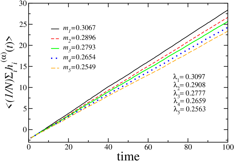
Figure 1: (Color online) Evolution of the mean height of surfaces $\langle\bar{h}_{\alpha}(t)\rangle$ associated with small perturbations initialized along characteristic LVs with indices $\alpha=1,\ldots,5$ from top to bottom (FPU model, $N=32$ and energy density $\epsilon=10$). The curves are averages over 100 realizations. The fitting slopes $m_{\alpha}$ are in good agreement with the corresponding values of $\lambda_{\alpha}$.

The main LV ${\mathbf{g}}_{1}={\mathbf{b}}_{1}$ in spatio-temporal chaotic systems is strongly localized in space kaneko86 ; giaco91 ; falcioni91 , and transformation (4) allows to unfold the spatial structure of the vector, which would be otherwise hidden close to zero. The localization of the main LV is dynamic, i.e. there is a slow wandering of the localization region. In Ref. pik01 it was demonstrated by means of numerical simulations that, contrary to dissipative systems and other systems with STC, the surface associated with ${\mathbf{g}}_{1}$ does not fall into the universality class of the KPZ equation. This fact is attributed to the presence of long-range correlations in space and time in Hamiltonian lattices pik01 .

For the FPU model we depict snapshots of surfaces corresponding to the first and second LVs in Figs. 2 (a) for the BLVs and (b) for CLVs. The vectors are strongly localized; notice that $h^{(\alpha)}_{i}$, Eq. (4), is a logarithmic variable. In Figs. 2(c,d), we plot the time evolution of the localization sites corresponding to BLVs and CLVs, for $\alpha=1,\ldots,10$. We define the localization site as the position $i$ where $h^{(\alpha)}$ takes its largest value at a given time. It can be readily seen that the maxima corresponding to the BLV-surfaces are scattered all over the spatial domain, just as in the case of the coupled-map-lattice (CML) studied in Ref. szendro07 where it was argued that this behavior is a byproduct of the orthogonalization procedure and not a physical property of the perturbation dynamics. On the contrary, CLVs present much more correlated localization sites.

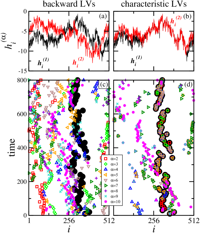
Figure 2: (Color online). (a,b) Snapshot of the LV-surfaces corresponding to $\alpha=1,2$ for the FPU lattice with $N=512$. (c,d) Space-time evolution of the localization sites for the first 10 LVs. The position of the localization site for the main LV is indicated by filled circles. Other symbols correspond to $\alpha=2,\ldots,10$.

The scaling properties of LVs corresponding to LEs smaller than the first one have been recently reported for spatio-temporally chaotic dissipative systems szendro07 ; pazo08 . These works revealed that LV-surfaces are piecewise copies of the main one. This is readily seen defining the difference-field

$$\eta_{i}^{(\alpha)}\equiv h_{i}^{(\alpha)}-h_{i}^{(1)}.$$ (5)

We show in Fig. 3, using CLVs, that this qualitative feature holds for Hamiltonian lattices as well (it is irrelevant that the first LV does not belong to the KPZ universality class). As in dissipative systems szendro07 ; pazo08 , the typical plateau size of $\eta^{(\alpha)}$ decreases as $\alpha$ grows, and beyond some $\alpha_{\mathrm{max}}$ this simple picture does not hold: Figure 3(b) shows that for $\alpha=8$ the plateaus are smaller than for $\alpha=2$, Fig. 3(a).

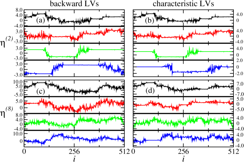
Figure 3: (Color online) Snapshots of the field $\eta_{i}^{(2)}$ at four different times for (a) backward LVs and (b) characteristic LVs. (c,d) Same as (a,b) but for the field $\eta_{i}^{(8)}$. Note that the typical length of the plateaus is smaller in this case. (FPU model with $N=512$ and $\epsilon=10$.)

IV spatial structure

In this section we perform a quantitative description of the spatial correlations of the LV-surfaces $h_{i}^{(\alpha)}(t)$. We compute the stationary structure factor $S_{\alpha}(k)=\lim_{t\rightarrow\infty}\langle\hat{h}^{(\alpha)}(k,t)\hat{h}^{(\alpha)}(-k,t)\rangle$, where $\hat{h}^{(\alpha)}(k,t)=N^{-1/2}\sum_{j}\exp(2\pi\imath\,k\,j)h_{j}^{(\alpha)}(t)$, with $\langle\ldots\rangle$ indicating an average over different system trajectories (which correspond to different random initial conditions).

Figures 4(a,b) and 5(a,b) show the structure factors of a representative set of LV-surfaces for FPU and $\Phi^{4}$ models, respectively. For the main LV surface, $\alpha=1$, the short wavenumber scaling exponent $\gamma$ of the structure factor ($S(k)\sim k^{\gamma}$) is clearly different from the one expected for the KPZ universality class in one dimension ($\gamma=-2$) and the obtained values, $\gamma=-2.5$ (FPU) and $\gamma=-2.6$ ($\Phi^{4}$), are consistent with those reported by Pikovsky and Politi pik01 .

As explained in Sec. II.2, for $\alpha>1$ one must distinguish between backward and characteristic LVs. Figures 4(a,b) and 5(a,b) evidence that both vector types indeed have different spatial structures. The structure factors of BLV-surfaces asymptotically decay with exponents $\gamma=-0.9$ (FPU) and $\gamma=-1.1$ ($\Phi^{4}$), which are close to the value $\gamma=-1$ reported for dissipative systems in Refs. szendro07 ; pazo08 . These results suggest that the value $\gamma\approx-1$ for BLVs in our Hamiltonian systems has a geometric origin and is related to the Gram-Schmidt orthonormalization. However, CLVs display exponents $\gamma=-1.4$ (FPU) and $\gamma=-1.3$ ($\Phi^{4}$) which, at least for the FPU model, are different from the values $-1.2$ or $-1.15$ reported in dissipative systems szendro07 ; pazo08 .

The fact that LVs corresponding to the most expanding directions are (in the surface representation) piecewise copies of the main LV translates into the existence of crossover wavenumbers where the structure factors bend. Each structure factor $S_{\alpha}$ presents a knee at a certain wavenumber $k_{\alpha}^{\times}$ that is related to the typical plateau length of the difference field $\eta^{(\alpha)}$. For both, FPU and $\Phi^{4}$, models $k_{\alpha}^{\times}$ scales with $\alpha$ approximately as $k_{\alpha}^{\times}\sim\left[(\alpha-1/2)/N\right]^{\theta}$, with $\theta\approx 1$ (as in Ref. szendro07 for a dissipative CML). We choose to use $\alpha-1/2$ instead of $\alpha$, as it is customary when plotting the Lyapunov spectrum (this is actually irrelevant in the thermodynamic limit $N\to\infty$). This is verified in Figs. 4(c,d) and 5(c,d) through a data collapse of the structure factors via the scaling relation

$$S_{\alpha}(k)k^{-\gamma}=g(k/k_{\alpha}^{\times}),$$ (6)

where $g(u)=$const for $u\gg 1$ and $g(u)\sim u^{\sigma}$ for $u\ll 1$.

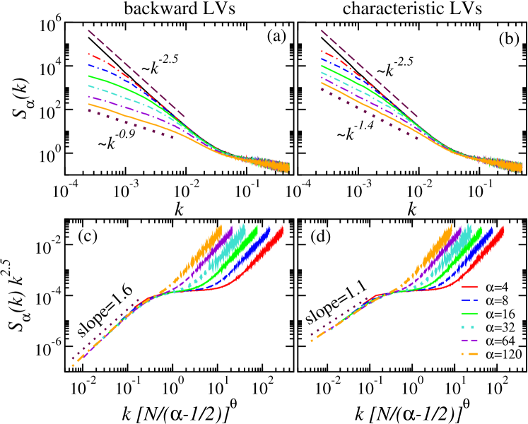
Figure 4: (Color online) Structure factors $S_{\alpha}(k)$ of the FPU model with $N=4096$, for (a) backward and (b) characteristic LV-surfaces, $\alpha=1,4,8,16,32,64,120$ from top to bottom. (c,d) Data collapse through scaling relation (6) with $\gamma=-2.5$ and fitting parameters $\theta=0.9$ (c) and $\theta=0.8$ (d); index $\alpha$ increases from right to left.

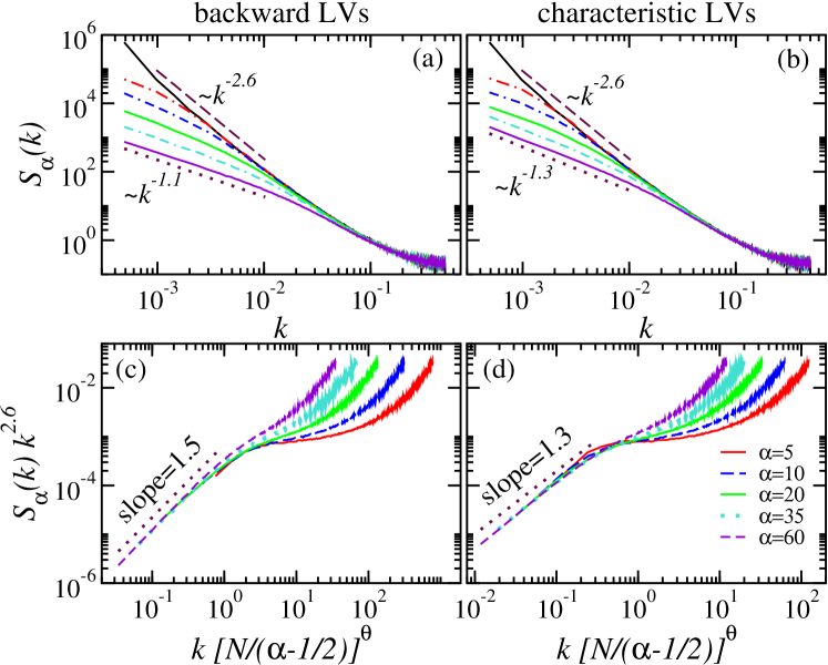
Figure 5: (Color online) Structure factors $S_{\alpha}(k)$ of the $\Phi^{4}$ model with $N=2048$, for (a) backward and (b) characteristic LV-surfaces, $\alpha=1,5,10,20,35,60$ from top to bottom. (c,d) Data collapse through scaling relation (6) with $\gamma=-2.6$ and fitting parameters $\theta=1.2$ (c) and $\theta=1.0$ (d); index $\alpha$ increases from right to left.

V discussion and conclusions

In a recent paper pazo08 we established (as suggested by pik98 ) a minimal stochastic model for LVs $w(x,t)$ in spatiotemporal chaos:

$$\partial_{t}w(x,t)=\xi(x,t)w(x,t)+\partial_{xx}w(x,t),$$ (7)

where $\xi(x,t)$ is a white noise term that accounts for the chaotic fluctuations. The generic asymptotic solution of Eq. (7) models the main LV, whereas “saddle solutions” (see pazo08 for details) correspond to CLVs with $2\leq\alpha\leq\alpha_{\mathrm{max}}$. This correspondence between a (linear) stochastic equation and LVs is supported by the existence of common scaling exponents pazo08 . The generic solution of (7) has the same sign in all the domain, and this allows to transform Eq. (7) into the KPZ equation through the Hopf-Cole transformation $h(x,t)=\ln|w(x,t)|$. In contrast, the saddle-solutions of (7) vanish at several points, what precludes KPZ as a valid equation for CLVs other than for $\alpha=1$.

In Hamiltonian systems, the anomalous scaling exponent ($\gamma\neq 2$) of the main LV was traced back pik01 to the long-range correlations of the multipliers driving the linear equations (2). For Hamiltonians of the form (1), these multipliers are functions of the displacements $\{q_{i}\}$ with specific properties for FPU and $\Phi^{4}$ models. The minimal model proposed in pik01 for the main LV-surface was the KPZ equation [or (7) reversing the Hopf-Cole transformation] with long-range correlated noise. Unfortunately, theoretical expressions for $\gamma$ medina89 ; Barabasi consider the KPZ equation with either spatially or temporally-correlated noise (but not both). The exponent $\gamma$ may take the same value with different combinations of spatial and temporal long-range correlations. Hence there is not a univocal relation between correlations and $\gamma$.

Minimal models are important as they are more amenable to theoretical analysis, which should allow to distinguish different universality classes. Our present work has the value of giving more constraints to the minimal stochastic model for perturbations in Hamiltonian lattices. A minimal model should reproduce the scaling properties of both the main LV and sub-dominant LVs. These sub-dominant ($\alpha\geq 2$) LVs have been the subject of the present study. A possible alternative to (7) pointed out in pik98 is the time-reversible equation:

$$\partial_{tt}w(x,t)=\xi(x,t)w(x,t)+\partial_{xx}w(x,t).$$ (8)

Future work is need to find out the true minimal model for LVs in Hamiltonian lattices. In any case, our results should be a guidance in the search of such a minimal model for Hamiltonian systems, since any suitable minimal model must produce surfaces with the scaling properties in Figs. 4 and 5.

Finally, a bit reversible algorithm, which operates with integer arithmetic, has been implemented to take advantage of the time reversibility of Hamiltonian systems. Although trajectory reversibility is not strictly required to compute the CLVs (in previous works szendro07 ; pazo08 CLVs have been computed in non-reversible dissipative systems), our methodology makes use of the aforementioned reversibility to completely bypass the need to store the phase-space trajectory in order to maximize the efficiency of the computation of the CLVs from the intersection of backward and forward LV subspaces if only limited computer resources are available.

Appendix A Bit reversible algorithm

Since the so called ‘bit reversible’ technique has been so far implemented using the standard Verlet integrator (which does not considers the momenta explicitly) and employed mainly for studies of time reversibility in Lennard-Jones fluids Verlet ; Romero ; Komatsu , (although it has also been applied in cases in which the so-called smoothed-particle continuum mechanics becomes isomorphic to molecular dynamics, see Ref. Hoover ) we will give a brief explanation of its current implementation in order to make this paper self-contained. Starting from the initial condition ${\mathbf{\Gamma}}(0)$, the phase-space point ${\mathbf{\Gamma}}(\Delta t)$ is obtained by means of the symmetrical velocity Verlet integrator Tuck written, in floating-point arithmetic, as

$$p_{i}\left(\frac{\Delta t}{2}\right) = p_{i}(0)+\frac{\Delta t}{2}F_{i}[q_{i}(0)],$$ (9a)

$$q_{i}(\Delta t) = q_{i}(0)+\frac{\Delta t}{m_{i}}p_{i}\left(\frac{\Delta t}{2}\right),$$ (9b)

$$p_{i}(\Delta t) = p_{i}\left(\frac{\Delta t}{2}\right)+\frac{\Delta t}{2}F_{i}[q_{i}(\Delta t)],$$ (9c)

where $F_{i}$ is the total force on the $i$th oscillator. The bit reversible version of algorithm (9) employs an integer representation of phase space instead of the conventional continuous phase space. To accomplish such transformation, for the considered lattices the minimum distance by which the phase space is discretized is defined as $\Delta L=N/2^{n}$, where $N$ is the system size and $2^{n}$ is the largest integer value if $n$-bit integers are employed. Because of the discretization, the phase space coordinates are represented by integers, i.e. $\{\mathbf{iq},\mathbf{ip}\}$. Therefore the evolution equations can be recast in the following form:

$$\mathrm{ip}_{i}\left(\frac{\Delta t}{2}\right) = \mathrm{ip}_{i}(0)+\sum_{j=i-1}^{i+1}\left\{\frac{\Delta t}{2}F_{ij}[q_{i}(0)]\right\}_{\mathrm{Integer}},$$ (10a)

$$\mathrm{iq}_{i}(\Delta t) = \mathrm{iq}_{i}(0)+\left\{\frac{\Delta t}{m_{i}}p_{i}\left(\frac{\Delta t}{2}\right)\right\}_{\mathrm{Integer}},$$ (10b)

$$\mathrm{ip}_{i}(\Delta t) = \mathrm{ip}_{i}\left(\frac{\Delta t}{2}\right)+\sum_{j=i-1}^{i+1}\left\{\frac{\Delta t}{2}F_{ij}[q_{i}(\Delta t)]\right\}_{\mathrm{Integer}},$$ (10c)

where $F_{ij}$ is a partial force from the $j$-th nearest neighbor on the $i$-th oscillator. It should be noted that the discrete coordinates $\{\mathbf{iq}(t),\mathbf{ip}(t)\}$ are integers, and the actual phase-space coordinates are obtained as $\mathbf{q}(t)=\mathbf{iq}(t)\Delta L$ and $\mathbf{p}(t)=\mathbf{ip}(t)\Delta L$. The second terms in the right hand side of Eqs. (10) are calculated based on the continuous phase space variables $\{\mathbf{q},\mathbf{p}\}$ and the values in brackets $\{\cdot\}_{\mathrm{Integer}}$ are converted to integers; in this way the total momentum is exactly zero at all times during the simulation Verlet .

With the aforementioned implementation time reversibility is achieved exactly throughout the simulations performed, which were rather long. To give an example, for the $\Phi^{4}$ model a simulation of $5\times 10^{8}$ time steps, after a transient of $1.5\times 10^{8}$, was needed to obtain the reported results. The situation is definitely better for the FPU model, where only $5\times 10^{6}$ time steps, with a transient of $5\times 10^{5}$, were sufficient for the employed system size. Due to the conversion process to integer, energy is not exactly conserved. Nevertheless, the exact-time-reversibility of the integration algorithm precludes any systematic drift in the total energy. We have confirmed that the fluctuation of the total energy by the bit reversible simulations is equivalent to that by conventional floating-point simulations.

References

- (1) E. Ott, Chaos in Dynamical Systems (Cambridge University Press, Cambridge, 1993).
- (2) R. Livi, A. Politi, and S. Ruffo, J. Phys. A: Math. Theor. 19, 2033 (1986).
- (3) R. Livi, A. Politi, S. Ruffo, and A. Vulpiani, J. Stat. Phys. 46, 147 (1987).
- (4) H.-L. Yang and G. Radons, Phys. Rev. E 73, 066201 (2006).
- (5) M. Romero-Bastida and E. Braun, J. Phys. A: Math. Theor. 41, 375101 (2008).
- (6) G. P. Morriss and D. Truant, J. Stat. Mech. P02029 (2009).
- (7) Y. Pomeau, A. Pumir, and P. Pelee, J. of Stat. Phys. 37, 39 (1984).
- (8) D. A. Egolf, I. V. Melnikov, W. Pesch, and R. E. Ecke, Nature 404, 733 (2000).
- (9) E. Kalnay, Atmospheric Modeling, Data Assimilation and Predictability (Cambridge University Press, Cambridge, 2002).
- (10) D. Pazó, M. A. Rodríguez, and J. M. López, Tellus 62A, 10 (2010).
- (11) A. S. Pikovsky and J. Kurths, Phys. Rev. E 49, 898 (1994).
- (12) A. Pikovsky and A. Politi, Nonlinearity 11, 1049 (1998).
- (13) M. Kardar, G. Parisi, and Y.-C. Zhang, Phys. Rev. Lett. 56, 889 (1986).
- (14) J. M. López, C. Primo, M. A. Rodríguez, and I. G. Szendro, Phys. Rev. E 70, 056224 (2004).
- (15) C. Primo, M. A. Rodríguez, J. M. López, and I. G. Szendro, Phys. Rev. E 72, 015201(R) (2005).
- (16) C. Primo, I. G. Szendro, M. A. Rodríguez, and J. M. López, Europhys. Lett. 76, 767 (2006).
- (17) D. Pazó, J. M. López, and M. A. Rodríguez, Phys. Rev. E 79, 036202 (2009).
- (18) A. Pikovsky and A. Politi, Phys. Rev. E 63, 036207 (2001).
- (19) I. G. Szendro, D. Pazó, M. A. Rodríguez, and J. M. López, Phys. Rev. E 76, 025202(R) (2007).
- (20) D. Pazó, I. G. Szendro, J. M. López, and M. A. Rodríguez, Phys. Rev. E 78, 016209 (2008).
- (21) B. Legras and R. Vautard, in Proc. Seminar on Predictability Vol. I, ECWF Seminar, edited by T. Palmer (ECMWF, Reading, UK, 1996), pp. 135–146.
- (22) D. Ruelle, Publ. Math. IHES 50, 27 (1979).
- (23) K. A. Takeuchi, F. Ginelli, and H. Chaté, Phys. Rev. Lett. 103, 154103 (2009).
- (24) F. Ginelli et al., Phys. Rev. Lett. 99, 130601 (2007).
- (25) P. V. Kuptsov and S. P. Kuznetsov, Phys. Rev. E 80, 016205 (2009).
- (26) H. L. Yang and G. Radons, Phys. Rev. Lett. 100, 024101 (2008).
- (27) H. L. Yang, K. A. Takeuchi, F. Ginelli, H. Chaté, and G. Radons, Phys. Rev. Lett. 102, 074102 (2009).
- (28) P. V. Kuptsov and U. Parlitz, Phys. Rev. E 81, 036214 (2010).
- (29) E. Fermi, J. Pasta, and S. Ulam (with M. Tsingou), Collected papers of Enrico Fermi (University of Chicago Press, Chicago, 1965), p. 978.
- (30) M. Pettini and M. Landolfi, Phys. Rev. A 41, 768 (1990).
- (31) M. Pettini and M. Cerruti-Sola, Phys. Rev. A 44, 975 (1991).
- (32) V. I. Oseledec, Trans. Moscow Math. Soc. 19, 197 (1968).
- (33) G. Benettin, L. Galgani, A. Giorgilli, and J.-M. Strelcyn, Meccanica 15, 9 (1980).
- (34) I. Shimada and T. Nagashima, Prog. Theor. Phys. 61, 1605 (1979).
- (35) S. V. Ershov and A. B. Potapov, Physica D 118, 167 (1998).
- (36) J.-P. Eckmann and D. Ruelle, Rev. Mod. Phys. 57, 617 (1985).
- (37) M. Tuckerman, B. J. Berne, and G. J. Martyna, J. Chem. Phys. 97, 1990 (1992).
- (38) C. L. Wolfe and R. M. Samelson, Tellus 59A, 355 (2007).
- (39) K. Kaneko, Physica D 23, 436 (1986).
- (40) G. Giacomelli and A. Politi, Europhys. Lett. 15, 387 (1991).
- (41) M. Falcioni, U. M. B. Marconi, and A. Vulpiani, Phys. Rev. A 44, 2263 (1991).
- (42) E. Medina, T. Hwa, M. Kardar, and Y.-C. Zhang, Phys. Rev. A 39, 3053 (1989).
- (43) A.-L. Barabási and H. E. Stanley, Fractal Concepts in Surface Growth (Cambridge University Press, Cambridge, 1995).
- (44) B. Hu, B. Li, and H. Zhao, Phys. Rev. E 61, 3828 (2000).
- (45) D. Levesque and L. Verlet, J. Stat. Phys. 72, 519 (1993).
- (46) V. Romero-Rochin and E. González-Tovar, J. Stat. Phys. 89, 735 (1997).
- (47) N. Komatsu and T. Abe, Physica D 195, 391 (2004).
- (48) O. Kum and W. G. Hoover, J. Stat. Phys. 76, 1075 (1994).