Calibration of the TWIST high-precision drift chambers

Abstract

A method for the precise measurement of drift times for the high-precision drift chambers used in the TWIST detector is described. It is based on the iterative correction of the space-time relationships by the time residuals of the track fit, resulting in a measurement of the effective drift times. The corrected drift time maps are parametrised individually for each chamber using spline functions. Biases introduced by the reconstruction itself are taken into account as well, making it necessary to apply the procedure to both data and simulation.

The described calibration is shown to improve the reconstruction performance and to extend significantly the physics reach of the experiment.

1 Introduction

The TRIUMF Weak Interaction Symmetry Test (TWIST) experiment measures momentum and angle distributions of positrons from the decay of highly polarised positive muons to obtain an accurate measurement of the decay parameters.

High-precision planar drift chambers are employed to reconstruct the positron tracks in the momentum and polar angle range of $15\lesssim p\lesssim 55$ MeV/$c$  and $0.5\lesssim|\cos\theta|\lesssim 1.0$, respectively. The chambers are contained in a solenoidal spectrometer with a 2 T magnetic field, and arranged symmetrically around a central target foil that stops the low energy muon beam (Fig. 1). Following the decay of the muon, the positron is tracked in the chambers and a high statistics decay distribution is acquired. The decay parameters are then extracted by comparing the measured spectrum with a simulation.

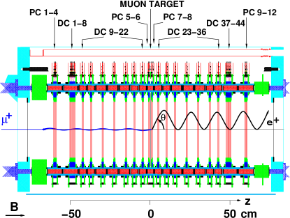
Figure 1: (Colour on-line.) Side view of the TWIST detector. It consists of two symmetric stacks of drift and proportional chambers (DCs and PCs) surrounding the muon stopping target and is immersed in a 2 T magnetic field. A typical event is shown with the helical track of the decay positron.

TWIST’s physics goal is an improvement in the accuracy of the decay parameters by one order of magnitude over previous measurements. Intermediate results, obtained from data taken before 2005, have been published [1, 2, 3, 4]. To further reduce the uncertainties for the analysis of the final data sets acquired in Oct-Dec 2006 and May-Aug 2007, a detailed understanding of the response of the drift chambers, in particular the space-time relationships (STRs), was required.

While the determination of drift time maps is a common problem, the chamber setup and the precision requirements for TWIST made it necessary to calculate accurate STRs directly from data. Consequently, a method was devised to measure the drift times individually for each chamber, taking into account construction inaccuracies, environmental parameters and interplay with the track reconstruction algorithms.

2 TWIST Drift Chambers

The 44 planar drift chambers (DCs) are the main tracking devices of the TWIST spectrometer. A more complete description of the design and construction of the DCs than is given here can be found in [5].

2.1 Chamber Design

A primary design requirement for the DCs was to minimise their total thickness, thereby reducing the amount of material that particles have to cross when passing through the detector. This minimises the uncertainties from the calculation of energy loss and multiple scattering. At the same time, the chambers had to obtain single-hit reconstruction efficiencies of above 99% and a spatial resolution of significantly better than 100 $\mu$m  to achieve the physics goals of the experiment.

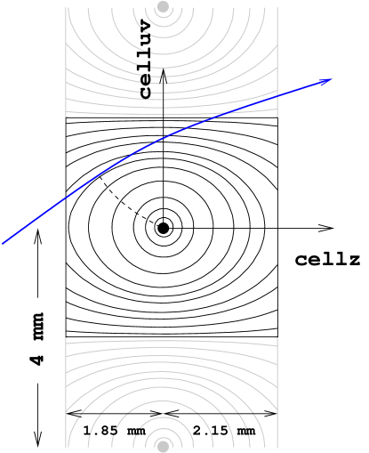
Figure 2: (Colour on-line.) Schematic layout of one drift cell and a projected particle trajectory. The cell coordinate system is defined with the origin at the wire and $cellz$ and $celluv$ ranging from -1.85 to 2.15 mm, and -2.00 to 2.00 mm, respectively. The isochrones for drift times of 2, 5, 10, 25, 50, 75, 100, 150, 200, 300, 500 ns are shown. As can be seen, the point of the charge deposit that reaches the wire first depends on the entry point and angle of the track. Its approximate path to the wire is indicated.

An individual chamber is composed of two parallel cathode foil discs of 320 mm radius, separated by 4 mm, and a wire plane with 80 parallel sense wires stretched across the disc at a pitch of 4 mm. The foils are located at 1.85 and 2.15 mm distance, defining asymmetric half-cells. No field wires are used. The schematic layout of one drift cell is shown in Fig. 2. A drift cell is defined as the projection of the drift space along all wires of a particular plane. Sense wires are 15 $\mu$m  diameter gold-plated tungsten/rhenium with the initial distance between wires accurate to approximately 3.3 $\mu$m  and the absolute wire positions known to better than 20 $\mu$m. The foils are aluminised Mylar with a nominal thickness of 6.35 $\mu$m. As drift gas dimethyl ether (DME) at atmospheric pressure is used. In addition to having a low mean atomic number, DME has a small Lorentz angle, a good cluster yield ($\approx$30 cm^-1) and a relatively low drift velocity, with the maximum drift times being below 1 $\mu$s for the given geometry.

2.2 Stack Assembly

As shown in Fig. 1 most DCs are assembled into modules of two chambers, with the central cathode foil shared, and the outer foils serving as gas containment windows. The two wire planes of such a module are rotated by $\pm$ 45 degrees with the detector axis to reduce gravitational sag. The wire orientations then define the $u/v/z$ coordinate system, with $z$ being the detector axis. Fourteen such modules are symmetrically arranged around the target, with irregular spacing to reduce ambiguities in the reconstruction. At the very upstream and downstream these modules are complemented by two stacks of eight DCs that have all inner foils shared. Upstream and downstream DCs are flipped with respect to each other so that the smaller half-cell is always oriented toward the target. In addition, proportional chambers (PCs) surround the DCs at the very upstream and downstream end of the detector, and around the target. They provide trigger and timing information and are not used for the track fit.

The precise $z$-positioning of all modules is implemented with ceramic spacers that have an extremely low thermal expansion coefficient. They stabilise the distances between two wire planes to an accuracy of better than 5 $\mu$m. The positioning of the foils is accurate to about 100 $\mu$m  with respect to the wire planes and is expected to vary from chamber to chamber. The space between the individual chamber modules is filled with a (97:3) mixture of helium and nitrogen at atmospheric pressure.

2.3 Operation

The pressures of the DME and He/N input lines are carefully adjusted and monitored to avoid differential pressure that would bulge the cathode foils. In particular, fast temperature changes of the detector environment have to be avoided to allow the control systems to adapt. The dynamic bulging of the foils was not bigger than 35 $\mu$m at the centre and does not constitute a considerable source of reconstruction uncertainties.

With unavoidable variations in the atmospheric pressure the density of the drift gas varies as well. This effect is accounted for in the determination and usage of the STRs (see below).

The chambers operate at a voltage of 1950 V, providing efficiencies of above 99% with no significant risk of sparking. Signals on the wires of all chambers pass through preamps and post-amplifier-discriminators before being read out by LeCroy 1877 multi-hit TDCs with 0.5 ns time resolution.

2.4 Drift Times

Initially, the drift properties of the chambers have been studied using the GARFIELD [6] program. GARFIELD calculates the drift times expected for a given setup, including the specifications of the gas, and the electric and magnetic fields. While an accurate drift time map can be obtained this way, there are inevitable differences with the real chambers, arising from construction inaccuracies, local variations of the electric field, and temperature and pressure variations. The impact of each of these effects on the drift times can be quantified using GARFIELD with modified chamber parameters, however a comparison with the real drift times of all 44 chambers cannot be obtained this way. This lack of knowledge, although difficult to quantify, could represent significant systematic uncertainties in the final TWIST results.

Drift times can be determined by using calculations, or data from test beams or dedicated calibration runs. These calibrations are often simplified by a static and well determined geometry of the chambers, or a symmetric setup where the drift time is a function of the drift distance only. An additional simplification may arise from a limited topology (curvature, angle) of the tracks traversing the sensitive volume. Another source of STR biases is the simulation of the ionisation rate of the drift gas which determines the separation of primary ionisation clusters. These are simulated using a cluster spacing matched to the shape of the time spectrum from tracks passing very close to the sense wire. Lastly, the algorithm used to reconstruct hits (i.e. assigning a spatial coordinate to a drift time) and track fitting may introduce biases. If any of those biases are different for data and simulation, or for calibration and physics data, uncertainties on the physics results arise that are difficult to quantify.

To reach the precision needed to achieve TWIST’s physics goals all of the above-mentioned concerns had to be addressed: small variations in the geometry, hence the electric field, of the 44 chambers are expected, drift cells are asymmetric and a two-dimensional parametrisation of the drift times is required, temperature and pressure gradients may be present, and tracks cross the drift volume at a large variety of angles and curvatures. In addition, it is important that approximations that are made in the TWIST track reconstruction impact data and simulation in the same way.

3 Track Reconstruction

A certain interplay between features of the reconstruction, in particular the track fit, and STRs can be expected. While the reconstruction was not changed for the application of this calibration, it is important to understand the algorithms that are employed.

3.1 Pattern Recognition

To reconstruct a track, the DC hits —signal times on individual wires— are first grouped based on timing information from the PCs. A combinatorial, geometric pattern recognition is performed on the hits in such a time window to assign groups of hits to a potential track candidate. For each track candidate an initial helix fit is performed by approximating the position of hits by the crossing coordinates of a pair of hit $u$ and $v$ wires in a module along with the module’s $z$ position. This gives the starting values for the drift-time fit.

3.2 Helix Fitting

The drift-time fit is the simultaneous least-squares minimisation of the sum of drift distance residuals of all points and the scattering angles between them. The residuals are calculated by approximating the track’s trajectory through a drift cell by a parabola, and finding the point of minimum drift time along that track. This is the expected signal time for this track, and the difference to the measured time is the time residual $t_{\text{res}}$. It can be translated into a drift distance residual by swimming orthogonal to the isochrones (see Fig. 2) to find the distance corresponding to a time difference of $t_{\text{res}}$. In practise, the drift distance is only varied radially. This approximation is made for performance reasons, but introduces biases depending on the position of the hit in the cell, and therefore the track angle. Individual drift distance residuals are weighted by the chamber resolution at the point where the hit is placed and then added to the $\chi^{2}$ function to be minimised.

The shape of the resolution function used to weight residuals is given by the width of the time residual distributions for most parts of the drift cell. Close to the wire, an additional mechanism is employed to reduce the weight of points for which the so-called left-right (L-R) ambiguity is not resolved yet. In those cases, during the first few fit iterations the hit could still be placed on either side of the wire, leaving two realistic drift time minima.

The presence of multiple scattering is taken into account by allowing kinks [7] between track segments. Seven such segments are defined between the centres of DC modules. Kinks are added to the $\chi^{2}$ function, weighted by the expected scattering angle for the amount of material crossed. This reduces angle-dependent biases such as tracks being split into segments by the reconstruction due to a large-angle scatter. In addition, the helix fit is not a simple fit to a geometrical helix. In order to obtain better resolution and minimise biases, the average energy loss of the particle and hence the diminishing radius in the magnetic field is taken into account. The fit result, typically after 10-15 iterations, is the particle’s time, position and momentum vector at the chamber closest to the target that has contributed a hit.

3.3 Usage of Drift Times

Drift times are provided to the fitter in the form of one $t_{\text{drift}}(cellz,celluv)$ STR table per DC plane, with a uniform granularity of 10 $\mu$m  in each dimension. Since the distance between the wires does not significantly deviate from the design values, the electric field and the drift times are defined symmetrically along the $celluv$ axis. The same symmetry can not be applied along the $cellz$ axis as the distance between wires and foils is not symmetric, and is associated with a rather large uncertainty in the foil position.

During the actual fit, the STRs are used both to find the minimum drift time along a trajectory, and also to convert the drift time residual into a drift distance residual. These operations are executed several hundred times for each track and must be optimised to reduce the computing time needed. Thus, the STRs are not used directly as a lookup table, but rather parametrised and converted into formats suited to accelerate these two particular search patterns.

4 Creation of new STRs

Calibrated STRs are calculated in an iterative procedure starting from STRs calculated by GARFIELD. At each step the time residuals are accumulated as a function of the hit position within the cell. These are applied as a correction to the input STRs in order to calculate the drift time table for the next iteration. For data, this is done individually for each chamber while for MC all chambers are treated as one.

The procedure to create new STRs is described here in some detail as implementing these steps correctly has proven to be challenging, but critical to the success.

4.1 Determination of Time Residuals

For the analysis of time residuals the drift cell is divided into 1044 bins (sub-cells) ranging from a size of (100 $\mu$m  $\times$ 50 $\mu$m) near the wire to (200 $\mu$m)² at the edges. Using the symmetry about the $cellz$ axis, points with negative $celluv$ are mirrored, leaving 522 sub-cells for the range of -1.85 mm $<cellz<$ 2.15 mm and 0.0 mm $<|celluv|<$ 2.0 mm. For each of those sub-cells, time residuals are stored in a histogram with 1 ns binning. These distributions are approximately Gaussian and a two-stage fit is used to extract the peak. To populate all sub-cells sufficiently, approximately $300\times 10^{6}$ events are processed, accepting all successfully fit tracks within a momentum range of 10-55 MeV/$c$  and an angular range of 0.15 $<|\cos\theta|<$ 0.95.

The calibration is performed off-line, and can use any decay data destined for physics analysis. As such, data from various data-taking periods are investigated to establish that STRs only depend on gas density, and are the same for all data after density variations are accounted for (see below).

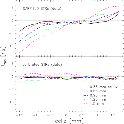
Figure 3: (Colour on-line.) Time residuals for an individual chamber (DC 2) before the calibration using GARFIELD STRs (top), and with the final calibrated STRs (bottom). The individual graphs are for various $celluv$ slices (c.f. Fig. 2) as indicated.

For most chambers the initial time residuals show a variety of distinct patterns, and can reach up to 15 ns in the corners of the drift cell (see Fig. 3 for a typical example). These time residuals quantify the difference between the real drift times and the ones calculated by GARFIELD, and represent the correction that needs to be made.

4.2 Fitting new STRs

Various methods have been explored for the parametrisation of the new STRs and the application of the correction defined by the time residuals. These are not straightforward, as the corrections are not measured in the same fine binning that is needed for the STR table, and the final STRs obviously need to satisfy certain smoothness and continuity requirements.

Under these conditions, STRs are most suitably represented by spline functions, and not by functional forms derived from theoretical considerations on the shape of the field. This is understandable considering that the helix fit algorithm introduces a small non-physical bias on its own, and given that the electric field itself might be deformed in a variety of shapes, resulting from deformations of the foils, for instance a tilt or bulge.

The best method for the subtraction of the time residuals was found to be the following algorithm. First, the fine-grained input STRs are down-sampled to the coarse binning of the time residuals so that the latter can simply be subtracted bin by bin. The resulting STR map is mirrored about the $cellz$ axis and fitted with a two-dimensional third order B-spline. To satisfy the boundary condition of $t_{\text{drift}}=0$ at the wire, a region of 250 $\mu$m  radius around the wire is blanked for the fit, and replaced with one individual highly weighted point at the wire and zero drift time. The resulting spline function is then used to calculate the drift time table for the 10 $\mu$m  grid used by the helix fitter.

The smoothness parameter for the spline fit is adapted individually for each plane in a compromise to obtain a close representation of the data points without introducing oscillations between points to which spline fits are prone. Other parameters, such as the number and position of knots of the spline are left free.

Before accepting a set of new STRs as basis for the next iteration, a test run is performed on a small amount of data. Several criteria are used to estimate whether these STRs represent an improvement over the previous iteration. The most direct indicator is a comparison of the distributions of the helix fit $\chi^{2}$: on average, the track fit residuals should obviously decrease, and more tracks should be reconstructed with a smaller $\chi^{2}$. In addition, the total number of successfully fit tracks should not decrease, while the computing time spent on an individual track fit should decrease. If these requirements are not met, this particular set of STRs is discarded and a new one is created, based on the same time residuals, by variation of the spline fit parameters. This procedure can easily require dozens of attempts, especially for data where the STRs for 44 planes need to be tuned individually, and no viable way of automation could be found.

4.3 Drift Gas Density Correction

Drift times are expected to vary with the density of the DME chamber gas. The pressure in the chambers is set to follow the atmospheric pressure, and together with inevitable changes in the environmental temperature this causes variations of the density. After a few iterations of the residual analysis described above, these variations manifest themselves in a time dependency of the drift time residuals. Time residual analyses of data from different time periods with significant differences in atmospheric pressure are used to parametrize the changes of drift times depending on the DME density. It is found to be consistent with predictions from GARFIELD and the maximal drift time variations are of the order of a few percent and the same for all planes and all parts of the drift cell. Consequently, for both the reconstruction and STR determination, input STRs are scaled according to the DME density based on temperature and atmospheric pressure measured for any given run, corresponding to a time frame of about 10 minutes. Other significant time-dependent variations of drift times have not been found. This is to be expected as long as the chambers remain mechanically unmodified.

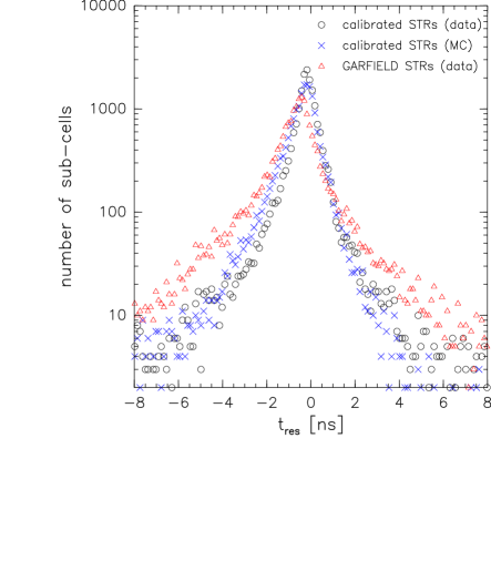
Figure 4: (Colour on-line.) Histograms of the time residuals of all sub-cells in the detector (44 planes times 522 sub-cells per plane). While there is still a slight difference between data and MC when calibrated STRs are used, a significant reduction of the tails are achieved. The latter are typically caused by asymmetries within the cell as shown in Fig. 3 and give rise to reconstruction biases.

4.4 Convergence

The procedure described above can be considered converged when no further improvement of track fit $\chi^{2}$ can be achieved. For MC, where all DC planes are the same, this typically requires 3-5 iterations. As a crosscheck, a plane by plane analysis was performed on MC to confirm that the algorithm itself does not introduce any significant plane-dependent bias. For data, about twice as many iterations are needed as considerable plane by plane variations need to be corrected. The time residuals at the end of the procedure are mostly within $\pm$ 1 ns, and no longer exhibit particular patterns that would lead to biases in the reconstruction (see Figs. 3, 4). In spatial coordinates, the correction can be quantified as up to 40 $\mu$m  in terms of shifts of individual isochrones.

On top of plane-dependent STRs, an analysis was performed to evaluate whether there are significant differences of time residuals in different regions of an individual DC plane. While minor differences were found, they were considered too small to warrant major efforts to correct. Moreover, unlike plane-to-plane differences, they should average out since the muon decay spectrum is rotationally invariant.

5 Resulting Improvements in the Analysis

The overall goal of any calibration in TWIST is to improve the consistency between data and MC. This is particularly important for the momentum and angle dependency of reconstruction biases, resolution and efficiencies. Such differences between data and MC would cause first order biases in the measured decay spectrum parameters and impact TWIST’s physics reach. While the possibilities of directly evaluating the above reconstruction benchmarks for data are very limited, some improvements to the track reconstruction as well as on decay parameters can be quantified as follows.

5.1 Track Fitting

Some features of the helix fits, such as residuals, the average number of points per track, the number of iterations, etc., can be used to evaluate the quality of the reconstruction, and to characterise how well the simulation represents the behaviour of the data. All of these benchmarks indicate that an improvement in the absolute performance as well as in the data-MC consistency is obtained. As an example the chamber resolution is shown in Fig. 5. It is derived from the width of the distribution of drift distance residuals of the helix fit for all planes. One can see that with the use of calibrated STRs the chamber resolutions for both data and simulation match within 5 $\mu$m  for most parts of the cell, compared to a systematic difference of up to 20 $\mu$m  before. With the hit position predominantly depending on the track angle, this reduces angle-dependent data-MC differences and also proves that the combined generation and reconstruction of hits is properly modeled in the MC.

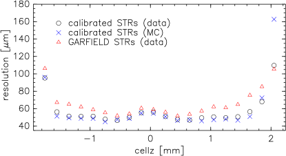
Figure 5: (Colour on-line.) Chamber resolution for a $celluv$ slice in the middle of the drift cell ($celluv$=0.95 mm). Using calibrated STRs for data allows the reconstruction to reach a similar resolution as for simulation. For the latter the reconstruction performance does generally not change significantly between using GARFIELD or calibrated STRs and only one of them is shown. The resolution achieved is roughly consistent with the 30-50 $\mu$m  predicted by GARFIELD and confirmed in bench tests of individual chambers (c.f. Fig. 15 of Ref. [5]).

The only test that directly allows a limited comparison of the momentum reconstruction bias and resolution in data and simulation is the evaluation of the kinematic edge of the spectrum at a momentum of $\approx$52.8 MeV/$c$. In the absence of physics beyond the Standard Model, its theoretical shape and position are known, and any smearing and shift of the reconstructed edge represents the momentum resolution and bias, respectively. At a fixed momentum, the resolution scales with the track radius and is proportional to $1/|\sin\theta|$. The value at $\theta=90^{\circ}$ can be used for comparisons and it is found that for both data and MC the momentum resolution is around $58\pm 1$ keV/$c$  while for previous analyses (e.g. [4]) it was typically 73 keV/$c$  in data and 69 keV/$c$  for MC. Similarly, calibrated STRs make the angular dependence of the momentum bias for data to be identical to the one in MC. These improvements lead to a more reliable energy scale calibration which is based on difference in the edge position between data and MC and has to be accurate to the level of a few keV/$c$.

5.2 Muon Decay Parameters

For most analyses completed prior to the development of the calibration described in this article, the dominant systematic uncertainty arose from the lack of knowledge of the STRs [1, 2, 4]: While for MC the same GARFIELD STRs were used for the generation and analysis, data was reconstructed with GARFIELD STRs that could not be validated conclusively against the real drift times.

The corresponding uncertainties were evaluated by the comparison of drift time spectra in data and MC, and later more accurately by using an early version of calibrated STRs. For the last pre-calibration analysis [4], the STRs were found to be the dominant source of uncertainties and increased the total systematic uncertainties of the experiment by up to 60%.

For the final TWIST analysis using calibrated STRs, the related uncertainties are estimated using the difference in the remaining time residuals between data and MC. They are found to be at least a factor of 5 smaller than before, and contribute less than 7% of the final systematic errors in the decay parameters. These significant improvements in the formerly leading systematic uncertainty are crucial to enable TWIST to reach its physics goals.

6 Summary

A method was devised to calibrate the space-time relationships of the TWIST high-precision drift chambers. It is based on an iterative procedure to correct drift time maps using the time residuals of the track reconstruction fit. Space-time-relationships are then parametrised by splines, individually for each of the planes in the detector. Differences between individual planes, as well as variations in operating conditions are corrected this way. The calibration is applied to data and simulation, reducing systematic differences such as reconstruction biases between both.

These improvements lead to a significant reduction of the related systematic uncertainties in the measurement of muon decay parameters that had limited previous analyses, and enable TWIST to extend its physics reach.

References

- [1] J. R. Musser et al. (TWIST), Phys. Rev. Lett. 94 (10) (2005) 101805.
- [2] A. Gaponenko et al. (TWIST), Phys. Rev. D 71 (7) 071101.
- [3] B. Jamieson et al. (TWIST), Phys. Rev. D 74 (7) (2006) 072007.
- [4] R. P. MacDonald et al. (TWIST), Phys. Rev. D 78 (2008) 032010.
- [5] R.S. Henderson et al., Nucl. Instrum. Methods A 548 (2005) 306.
- [6] R. Veenhof, Garfield: Simulation of gaseous detectorsVersion 7.10, CERN program Library long writeup W5050.
- [7] G. Lutz, Nucl. Instrum. Methods A 273 (1988) 349.