Sunyaev-Zel’dovich effects from annihilating dark matter in the Milky Way:
smooth halo, subhalos and intermediate-mass black holes

Abstract

We study the Sunyaev-Zel’dovich effect potentially generated by relativistic electrons injected from dark matter annihilation or decay in the Galaxy, and check whether it could be observed by Planck or the Atacama Large Millimeter Array (ALMA), or even imprint the current CMB data as, e.g., the specific fluctuation excess claimed from an recent reanalysis of the WMAP-5 data. We focus on high-latitude regions to avoid contamination of the Galactic astrophysical electron foreground, and consider the annihilation or decay coming from the smooth dark matter halo as well as from subhalos, further extending our analysis to a generic modeling of spikes arising around intermediate-mass black holes. We show that all these dark Galactic components are unlikely to produce any observable Sunyaev-Zel’dovich effect. For a self-annihilating dark matter particle of 10 GeV with canonical properties, the largest optical depth we find is $\tau_{e}\lesssim 10^{-7}$ for massive isolated subhalos hosting intermediate-mass black holes. We conclude that dark matter annihilation or decay on the Galactic scale cannot lead to significant Sunyaev-Zel’dovich distortions of the CMB spectrum.

I Introduction

The Sunyaev-Zel’dovich (SZ) effect stands for the distortion of the cosmic microwave background (CMB) spectrum by the scattering of thermal or relativistic electrons Sunyaev and Zeldovich (1972). In this paper, we aim at studying the SZ effect as a possible signature complementary to other indirect probes of dark matter annihilation on the Galactic scale (e.g. Gunn et al. (1978); Stecker (1978); Silk and Srednicki (1984); Silk et al. (1985); Srednicki et al. (1986); Turner (1986)), even though it was recently shown to be hardly observable for galaxy clusters Yuan et al. (2009); Lavalle et al. (2010). This study is partly motivated by the recent hint for $\sim 10^{\circ}$ angular scale SZ signals in the WMAP 5-year data away from the Galactic plane by Joudaki et al. (2010), potentially of Galactic origin, which might be explained by a column density of electrons of $\sim 10^{22}\,{\rm cm^{-2}}$, i.e. an optical depth as large as $\sim 10^{-3}$.

A simplistic comparison of the physical scales relevant to the calculation already provides some interesting information, since the SZ signal is roughly independent of the target distance (except for angular resolution effects). In galaxy clusters, the main contribution to the SZ signal, already difficult to observe to high precision, comes from a typical thermal electron density $n_{e}^{\rm th}\sim 10^{-2}\,{\rm cm^{-3}}$ integrated along a line-of-sight spatial scale $l\sim 500\,{\rm kpc}$. The SZ effect amplitude is roughly set by the electron optical depth $\tau_{e}\sim\sigma_{\rm T}\,n_{e}\,l$, where $\sigma_{\rm T}$ is the Thomson cross section. With the previous numbers we readily get $\tau_{e}\sim 10^{-3}$ for thermal electrons in clusters, consistent with most predictions (e.g. Birkinshaw (1999)), which provides a reference value for detectability. In the Milky Way, the typical relativistic electron density measured at the Earth, which constitutes a sound local upper bound to the yield potentially originating from dark matter annihilation at the GeV-TeV energy scale, is $\sim 10^{-11}-10^{-12}\,{\rm cm^{-3}}$ around 1 GeV (see e.g. Alcaraz et al. (2000)); this density can be associated with a typical spatial scale of a few tens of kpc for the bulk of usual dark matter density profiles. This translates into $\tau_{e}\lesssim 10^{-12}$ for relativistic Galactic electrons of energy $>1$ GeV. Although the lower energy part of the electron spectrum should play an important role (see the discussion in Sec. III.1), we could at zeroth order bet for no significant effect caused by dark matter annihilation or decay products at this stage.

Nevertheless, dark matter can collapse on scales as small as its free-streaming length at the twilight of the radiation era in the early universe, which is much smaller than the size of the Galactic halo for generic weakly interacting massive particles (WIMPs) (e.g. Bringmann (2009)). Such dark lumps are called subhalos and are commonly observed in N-body simulations of structure formation (e.g. Diemand et al. (2005)), though on scales larger than a few tens of pc due to numerical limits. This clustering implies a significant degree of inhomogeneity in the Galactic dark matter distribution which may lead to a global increase of the annihilation rate Silk and Stebbins (1993). This may consequently increase the electron density injected by dark matter annihilation over the entire Galaxy, and therefore along a given line of sight — in contrast, the effect is expected much less important for decaying dark matter for which the decay rate scales only linearly with its density, so that the global injection rate is fixed by the total mass of the Galaxy. Indeed, although it was shown that subhalos could not drastically enhance the local dark-matter-induced electrons Lavalle et al. (2008), the SZ effect is a cumulative effect along a line of sight which may therefore be more affected by subhalos, as it is the case for the complementary gamma-ray signals Bergström et al. (1999). Moreover, in addition to this class of inhomogeneities, other putative Galactic compact objects like intermediate-mass black holes (IMBHs) could raise spikes of dark matter Zhao and Silk (2005) and might also be able to seed SZ features in the CMB spectrum. It is not as straightforward as above to estimate the contributions of these different components, and it is consequently interesting to clarify this issue by means of explicit calculations, which we perform below.

The outline is the following. In Sec. II, we first focus on the basic physical parameter that sizes the amplitude of the CMB spectral distortion, i.e. the optical depth. In Sec. III, we calculate the optical depths for the smooth dark matter halo, and for both the resolved and unresolved subhalos. In Sec. IV, we briefly discuss the IMBH case, before concluding in Sec. V.

II Sizing the SZ amplitude: the electron optical depth

Dark matter annihilation in the GeV-TeV energy range leads to the injection of relativistic electrons. Interestingly enough, the SZ signal generated by these electrons should not suffer too much from the Galactic foreground if detected at sufficiently high latitude, since the astrophysical sources of electrons are expected to be concentrated in the Galactic disk. Moreover, no significant additional thermal SZ is expected to shield the potential dark matter contribution, in contrast to the galaxy cluster case.

Two different formalisms were developed to calculate the SZ effect, one based on radiative transfer (e.g. Wright (1979); Rephaeli (1995); Birkinshaw (1999); Enßlin and Kaiser (2000)), offering a nice analytical framework for thermal or relativistic electrons as long as the Thomson approximation is valid, and another relying on the covariant Boltzmann equation for which relativistic corrections to the thermal case were often obtained by means of Taylor expansion methods (e.g. Challinor and Lasenby (1998); Itoh et al. (1998)). In fact, these two formalisms were recently shown to be equivalent in the Thomson regime Bœhm and Lavalle (2009), in which analyticity is therefore preserved Bœhm and Lavalle (2009); Nozawa and Kohyama (2009). In the following, we use the formalism presented in Ref. Lavalle et al. (2010), to which we refer the reader for more details.

One of the most important physical parameters entering the SZ prediction is the so-called optical depth $\tau_{e}$ characterizing the electrons responsible for the spectral distortion of the CMB. Averaging it over the angular resolution $\delta\Omega$ of the detector, we have

$$\langle\tau_{e}\rangle_{\rm res} = \frac{\sigma_{\rm T}}{\delta\Omega(\mu_{\rm res})}\int_{\delta\Omega(\mu_{\rm res})}d\Omega\int dl\,n_{e}(\vec{x})\;,$$ (1)

where $dl$ denotes the line of sight, $\sigma_{\rm T}$ is the Thomson cross section, $n_{e}$ is the electron density in the target, $\mu_{\rm res}\equiv\cos(\theta_{\rm res})$ features the angular resolution $\theta_{\rm res}$. The typical optical depth leading to observable thermal SZ is $\tau_{e}\gtrsim 10^{-3}$ in galaxy clusters Birkinshaw (1999), which provides us with a benchmark value useful for further comparisons, while current and coming experiments can reach micro-Kelvin temperature fluctuations, or equivalently $\tau_{e}\sim 10^{-4}$ (e.g. The Planck Collaboration (2006); Science with ALMA (2008); Wootten and Thompson (2009)).

In the following, we compute the electron density $n_{e}$ expected for the different dark matter components introduced above.

III SZ from the annihilation products of the dark matter halo and subhalos

Electrons potentially injected in the Milky Way from dark matter annihilation or decay (say on the GeV-TeV energy scale) are expected to diffuse on small-scale moving magnetic turbulences and lose their energy through Compton interactions with the interstellar radiation fields (CMB is one of them) and the magnetic field, and through Coulomb interactions with the interstellar gas. For regions distant by more than a few kpc to the Galactic plane and almost devoid of interstellar gas and magnetic field, the main target for energy loss is the CMB. Nevertheless, independent of the peculiar regime, the transport equation that describes the evolution of the electron phase-space density after injection has to include all important processes — the associated general mathematical formalism is well established (e.g. Ginzburg and Syrovatskii (1964); Berezinskii et al. (1990)).

III.1 Galactic foreground

There exist many astrophysical sources of high-energy electrons in the Galactic disk, like supernova remnants or pulsars (see e.g. Delahaye et al. (2010) for a recent analysis of the local flux), which justifies to preferentially look for dark-matter-induced SZ signals at high Galactic latitude. The SZ foreground due to this specific population can be grossly assessed by slightly refining the argument discussed in the Introduction. The Fermi experiment has recently measured the flux of electrons in the energy range 10-1000 GeV Abdo et al. (2009); Pesce-Rollins and for the Fermi-LAT Collaboration (2009), which amounts to $\phi_{e}(E)\approx 2\times 10^{-5}(E/10\,{\rm GeV})^{-3}\,{\rm cm^{-2}s^{-1}sr^{-1}GeV^{-1}}$. This flux translates into a density of $dn_{e}^{\rm astro}(E)/dE\approx 8\times 10^{-15}(E/10\,{\rm GeV})^{-3}\,{\rm cm^{-3}GeV^{-1}}$. A naive integration of this power law down to 1 MeV provides a reference value of $n_{e}^{\rm astro}(>1\,{\rm MeV})\approx 4\times 10^{-6}\,{\rm cm^{-3}}$. Assuming that this density is constant up to $L\sim 5$ kpc in the direction perpendicular to the Galactic plane, which roughly corresponds to the vertical extent of the cosmic-ray confinement region, and vanishes beyond, we can derive an approximate optical depth of

$$\tau_{e,{\rm rel}}^{\rm astro}\approx\sigma_{\rm T}\,n_{e}^{\rm astro}\,L\approx 4\times 10^{-8}\;.$$ (2)

This gives an indication about the high-latitude contribution to the SZ of astrophysical relativistic electrons located close to the disk, which the dark matter yield in the same region cannot exceed too much without exceeding the local electron flux in the meantime. This is likely an overestimate since the astrophysical electron density is expected to decrease quite fast away from the disk, where most of the sources are located.

To complete the astrophysical foreground picture, we need to account for the thermal electron contribution. We take advantage of the well-known NE2001 model designed in Ref. Cordes and Lazio (2002) from pulsar dispersion measures, from which it is quite easy to numerically perform the line-of-sight integral perpendicular to the Galactic plane, from the Earth location. Taking the thin disk and thick disk components of this model, we find that

$$\tau_{e,{\rm th}}^{\rm astro}\approx 10^{-4}\;.$$ (3)

Thus, the local thermal astrophysical foreground is likely the dominant one, with a rather large amplitude. Such a value is actually not that surprising since it was already emphasized in Ref. Taylor et al. (2003) that the SZ flux generated by thermal electrons in nearby galaxies could be detected. Note that in the previous estimate, we did not include electrons from the very local interstellar medium nor from the nearby spiral arm, which we do not expect to significantly change this approximate result.

III.2 Dark matter contributions

III.2.1 Smooth-halo contribution

In contrast to high-energy electrons of astrophysical origin, dark-matter-induced electrons are produced everywhere in the Galactic halo, and the relevant line-of-sight length can therefore reach $\sim 100$ kpc. As briefly mentioned in the Introduction, the very simple exercise of using the local astrophysical electron density as a maximum for the dark matter-induced density at Galactic radii $r>\mbox{$r_{\odot}$}=8$ kpc would lead to $\tau_{e}\lesssim 8\times 10^{-11}$, rather far away from current experimental sensitivities. Nevertheless, it is worth quantifying more accurately the density distribution of the electrons injected by dark matter annihilation (or decay) along the line of sight in the high Galactic latitude regions.

The transport of electrons in regions distant from the disk is not very well constrained because it is difficult to predict the value of the diffusion coefficient. This latter should at least be much larger than locally because magnetic turbulences, somehow connected to small-scale inhomogeneities in the cosmic-ray plasma, are expected to fade away (e.g. Shalchi (2009)). In any case, the transport of electrons usually relies on a diffusion equation which can sometimes be solved in terms of analytical Green functions (see e.g.  Ginzburg and Syrovatskii (1964); Berezinskii et al. (1990) for extensive reviews, and Sec. III.2.5 for a few further details). In this context, the Green function ${\cal G}$ represents the probability for an electron injected at position $\vec{x}$ and energy $E_{s}$ to have propagated to position $\vec{x}$, still carrying energy $E\leq E_{s}$ (we only consider energy losses here), so that the electron density $dn/dE$ can be expressed in terms of a source ${\cal Q}$ as follows:

$$\frac{dn(E,\vec{x})}{dE}|_{\rm propag} = \int_{E}^{\infty}dE_{s}\int d^{3}\vec{x}_{s}\,{\cal G}(E,\vec{x}\leftarrow E_{s},\vec{x}_{s})$$ (4)

$$\times{\cal Q}(E_{s},\vec{x}_{s})\;.$$

As a minimal approach, which will be shown overoptimistic later on, we first neglect all processes but the energy losses caused by inverse Compton scattering with the CMB photons. If making such a maximal assumption, which greatly facilitates the calculation, is not enough to predict an observable SZ effect, then rather trustworthy conclusions can easily be drawn. We therefore suppose that electrons lose energy at their production site, i.e. we neglect spatial diffusion. In that case, referred to as diffusionless limit hereafter, the Green function ${\cal G}(E,\vec{x}\leftarrow E_{s},\vec{x}_{s})\longrightarrow\delta(\vec{x}_{s}-\vec{x})/b(E)$, such that the electron density at point $\vec{x}$ is related to the local annihilation rate as follows:

$$\frac{dn}{dE}(E,\vec{x})\approx\frac{1}{b(E)}\int_{E}^{\infty}dE_{s}\,{\cal Q}_{n}(E_{s},\vec{x})\;,$$ (5)

where the source term ${\cal Q}_{n}$ encodes the dark matter properties as

$${\cal Q}_{n}(E_{s},\vec{x})={\cal S}_{n}\left[\frac{\rho(\vec{x})}{\rho_{0}}\right]^{n}\,\frac{dN}{dE_{s}}\;.$$ (6)

Parameter $\rho_{0}$ denotes an arbitrary reference density and $dN/dE_{s}$ is the injected electron spectrum. The index $n$ is equal to 2 (1) in the case of dark matter annihilation (decay), for which the parameter ${\cal S}$ reads

$${\cal S}_{n}=\begin{cases}\frac{\Gamma_{\chi}\,\rho_{0}}{\mbox{$m_{\chi}$}}&n=1\\ \delta\frac{\mbox{$\langle\sigma v\rangle$}}{2}\left[\frac{\rho_{0}}{\mbox{$m_{\chi}$}}\right]^{2}&n=2\end{cases}\;.$$ (7)

We recognize the WIMP mass $m_{\chi}$, the annihilation cross section $\langle\sigma v\rangle$ and the decay rate $\Gamma_{\chi}$. The parameter $\delta$ is equal to 1 if annihilation involves identical WIMP particles, or to 1/2 for Dirac fermions.

For simplicity, we first consider annihilation or decay into electron-positron pairs, so that $dN/dE_{s}=2\,\delta(E_{s}-n\,\mbox{$m_{\chi}$}/2)$. Indeed, it is clear from Eq. (5) that the integrated electron density will mostly depend on the total number of electrons produced from dark matter annihilation or decay, so it will not be difficult to extrapolate the results obtained with this specific simple case to other injected spectra (as far as the optical depth is the only quantity under investigation and the diffusionless limit is considered). From this assumption, we obtain

$$n_{e}(\vec{x})={\cal S}_{n}\left[\frac{\rho(\vec{x})}{\rho_{0}}\right]^{n}\,\tau_{l}\,{\cal F}(E_{\rm min})\;,$$ (8)

where $\tau_{l}$ is the energy-loss timescale. In the Thomson approximation, the energy loss caused by interactions with the CMB is merely given by $b(E)=b_{0}(\epsilon\equiv E/E_{0})^{2}$ with $b_{0}=E_{0}/\tau_{l}=2.65\times 10^{-17}\,{\rm GeV/s}$, such that the integrated spectrum ${\cal F}$ can be expressed as

$${\cal F}(E_{\rm min})=2\,\,E_{0}\,\left(\frac{1}{E_{\rm min}}-\frac{2}{n\,\mbox{$m_{\chi}$}}\right)\simeq\frac{2\,E_{0}}{E_{\rm min}}\;.$$ (9)

In the following, we set $E_{0}$ to 1 GeV, which implies $\tau_{l}=3.8\times 10^{16}$ s. Note that neglecting other sources of energy loss, e.g. bremsstrahlung or ionization, is justified far away from the disk where the interstellar gas density is negligible.

We have now to specify the dark matter mass density shape $\rho(\vec{x})$. While there are still issues regarding how dark matter concentrates in the centers of galaxies, essentially because baryons dominate the central gravitational potential in these structures, the off-center regions are less subject to debate. Basically, N-body simulations agree on the prediction that the total dark matter density (including subhalos) should fall like $\sim r^{-3}$ in the outskirts of galaxies, which means that line-of-sight integrals should not differ too much among different Galactic halo models towards high-latitude regions. In the following, for comparison, we use the results of two recent high resolution N-body simulations of Milky-May-like objects, Via Lactea II Diemand et al. (2008) and Aquarius Springel et al. (2008a), in which the dark matter halos are found well approximated by spherical profiles; a summary of the relevant ingredients can be found in Pieri et al. (2009): the former is featured by a $r^{-1}$ Navarro-Frenk-White (NFW) profile Navarro et al. (1997) with a scale radius of $21$ kpc and a local mass density of $\rho(\mbox{$r_{\odot}$}=8\,{\rm kpc})=0.42\,{\rm GeV/cm^{3}}$, while the latter follows an Einasto profile with a slope $\alpha=0.17$, a scale radius of 20 kpc, and a local density of $0.57\,{\rm GeV/cm^{3}}$. Though different, these local normalizations are in reasonable agreement with the latest constraints to date Catena and Ullio (2010); Salucci et al. (2010).

In a spherical system centered about the Galactic center with an observer located at point $\vec{r}_{\odot}$, the vector running from the observer along the line-of-sight $\vec{l}$ and making an angle $\eta^{\prime}\equiv\pi-\eta$ with $\vec{r}_{\odot}$ can be related to the Galactic radius $r$ through $\vec{r}=\vec{r}_{\odot}+\vec{l}$, such that

$$r = \sqrt{l^{2}+r^{2}_{\odot}-2\,l\,r_{\odot}\,\cos\eta}$$ (10)

$$\Leftrightarrow l = r_{\odot}\,\cos\eta+\sqrt{r^{2}-r_{\odot}^{2}\,\sin^{2}\eta}\;.$$ (11)

This angle $\eta$ can actually be expressed in terms of the pointing angle of the telescope $\psi$ with respect to the Galactic center direction, the angle $\theta$ that describes the angular resolution, and the angle $\phi$ that runs circularly around the pointing direction,

$$\cos\eta=\sin\psi\,\sin\theta\,\cos\phi+\cos\theta\,\cos\psi\;.$$ (12)

Note that because of the spherical symmetry, $\psi$ merely corresponds to (minus) the Galactic latitude $b$ for an observer located on Earth, as measured at longitude $0^{\circ}$. Armed with these relations, we can readily compute the electron density at a given position $l$ along the line of sight, such that the optical depth averaged over the resolution angle $\theta_{\rm res}$ defined in Eq. (1) is finally given by

$$\langle\tau_{e,n}^{\chi}(\psi)\rangle_{\rm res}=\sigma_{\rm T}{\cal S}_{n}\,\tau_{l}\,{\cal F}(E_{\rm min})\,\left(2\,r_{0}\,{\cal J}_{n}(\psi,\mu_{\rm res})\right)\;,$$ (13)

where $\mu_{\rm res}=\cos(\theta_{\rm res})$. Similarly to what is encountered in indirect dark matter detection with gamma rays Bergström et al. (1998), we have defined the dimensionless parameter ${\cal J}$, the averaged line-of-sight integral, as follows:

$${\cal J}_{n}(\psi,\mu_{\rm res}) \equiv\frac{1}{4\,\pi\,r_{0}(1-\mu_{\rm res})}\,\times$$ (14)

$$\int_{0}^{2\pi}d\phi\int_{\mu_{\rm res}}^{1}d\mu\,\int_{0}^{\infty}dl\,\left[\frac{\rho(l(r,\psi,\mu,\phi))}{\rho_{0}}\right]^{n}\;.$$

We will further use $\rho_{0}=0.3\,{\rm GeV/cm^{3}}$ and $r_{0}=r_{\odot}=8$ kpc.

Figure 1: Plot of the parameter ${\cal J}_{\rm ann}\equiv J_{2}$ corresponding to the dark matter annihilation case [see Eq. (14)] for two configurations, the first one inspired from Via Lactea II Diemand et al. (2008) and the other one inspired from Aquarius Springel et al. (2008b). The dashed curves correspond to the smooth only contributions, the dash-dotted curves to the smooth approximation, the dotted curves to the subhalo contributions, and the solid curves the sum of the smooth-only and subhalo contributions.

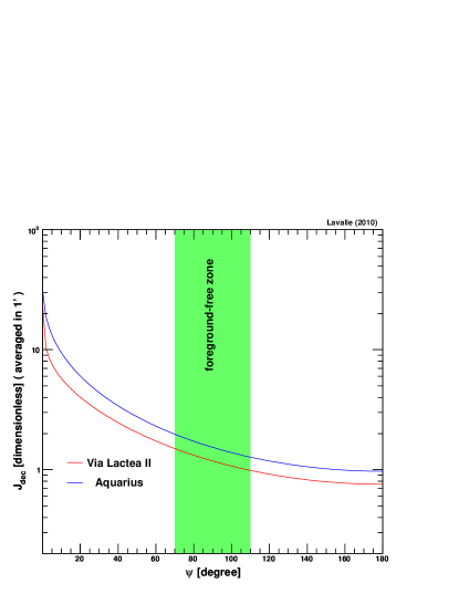
Figure 2: Plot of the parameter ${\cal J}_{\rm dec}\equiv J_{1}$ corresponding to the dark matter decay case (see Eq. 14) for the same two configurations as in Fig. 1. For dark matter decay, subhalos do not play any role in average.

The results obtained for the numerical calculation of ${\cal J}_{2}(\psi,\theta_{\rm res}=1^{\prime})$ are displayed in Fig. 1. The high-latitude zone corresponds to $70^{\circ}\lesssim\psi\lesssim 110^{\circ}$ (the colored region in the plot), for which the astrophysical foreground is expected to be the lowest. The dash-dotted curves represent the so-called smooth approximation for both the dark matter profiles discussed above, i.e. disregarding the potential presence of subhalos — their impact is discussed in Sec. III.2.2. The parameter ${\cal J}_{2}$ associated with the smooth dark matter halo is found $\lesssim 2$ in the region of interest (shaded). We find similar results on large latitudes for the dark matter decay case, as illustrated in Fig. 2.

To summarize, we provide a crude estimate of the optical depth in the smooth approximation. If we define

$$\bar{\cal N}^{\chi}_{n} \equiv \frac{\tau_{l}}{3.8\times 10^{16}{\rm s}}\,\frac{{\cal S}_{n}}{1.35\times 10^{-27}{\rm cm^{-3}s^{-1}}}$$

$$\times\frac{{\cal F}(m_{e})}{2/(511\times 10^{-6})}\,\frac{r_{0}\times{\cal J}_{n}}{8\,{\rm kpc}\times 2}\;,$$

which is equal to $\delta$ — i.e. 1 or 1/2 [see Eq. (7)] — (or 1) for the canonical values of the parameters made explicit above in the case of dark matter annihilation (decay, respectively). The reference value given above for ${\cal S}_{n}$ was obtained by assuming $\mbox{$\langle\sigma v\rangle$}=3\times 10^{-26}{\rm cm^{3}/s}$ (n=2, annihilation) or $\Gamma_{\chi}=4.5\times 10^{-27}{\rm s^{-1}}$ (n=1, decay), for $\mbox{$m_{\chi}$}=1$ GeV and $\rho_{0}=0.3\,{\rm GeV/cm^{3}}$ [see Eq. (7)]. The average optical depth is then approximately

$$\langle\tau_{e,n}^{\chi}(90^{\circ})\rangle_{1^{\prime}}=1.3\,10^{-8}\bar{\cal N}^{\chi}_{n}\;.$$ (16)

This value, which roughly sizes the amplitude of the SZ signal expected from high latitudes, is very small, much smaller than the typical optical depth found for Galactic thermal electrons and, more importantly, than the current experimental sensitivities. Indeed, we recall that new generation experiments, like Planck The Planck Collaboration (2006) or ALMA Science with ALMA (2008); Wootten and Thompson (2009), can hardly constrain electron populations of optical depths $\lesssim 10^{-4}$. We emphasize that we used a rather light WIMP mass of 1 GeV in this estimate (see e.g. Bœhm and Fayet (2004); Bœhm et al. (2004) for more detailed phenomenological aspects on light dark matter) and considered the favorable case of a diffusionless “transport” for electrons. Likewise, we employed a value of ${\cal F}$ down to the rest energy of electrons, and a reasonable angular resolution of $1^{\prime}$ — the angular resolution does not play a significant role when the line of sight is offset from the center of the target structure. These optimal assumptions still lead to a weak result, comparable with what we obtained for the relativistic astrophysical foreground but much smaller than the thermal one [see Eqs. (2) and (3)], which makes the SZ effect a too feeble tracer of dark matter annihilation or decay for a smooth Galactic halo.

A larger amplitude could be reached with lighter dark matter particles, but additional astrophysical constraints, e.g. coming from hard x-ray observations of the Galactic center Knödlseder et al. (2005), may then bound the annihilation cross section to smaller values as well Boehm et al. (2004); Ascasibar et al. (2006). The presence of dark matter substructures could also increase the amplitude in the case of dark matter annihilation, which is precisely the topic of the next paragraph. Note that for dark matter decay, subhalos, which are small-scale inhomogeneities, are not expected to significantly boost the SZ signal because the decay rate scales linearly with the dark matter density: the above smooth-halo approximation is likely a rather good approximation in that case.

III.2.2 Subhalo contributions

So far, we have considered a spherical and smooth dark matter halo without discussing the role of subhalos (see Sec. III.2.2). In this section, we study two different cases: (i) the collective effect of a subhalo population and (ii) the impact of a single big subhalo located along the line of sight. We recall that subhalos are expected to play a more minor role in the case of dark matter decay.

III.2.3 Average subhalo contribution

Let us first assume that subhalos contribute another smooth injection of electrons, the rate of which is set by their inner properties averaged over their spatial and mass distributions. Subhalos are indeed usually described in terms of (i) their global properties, i.e. their mass and spatial distributions, and (ii) their inner properties, i.e. their mass $m$, mass density shape $\rho_{\rm sh}$, concentration $c$ and position $r$ in the host halo. Theoretical prescriptions can be found for both types from cosmological simulation results. Once the subhalo properties are fixed, the global associated annihilation rate can be calculated. Thus, the dimensionless ${\cal J}$ factor associated with the electron injection from a population of subhalos is given by

$${\cal J}_{\rm sh}(\psi) =\frac{N_{\rm sh}^{\rm tot}}{4\,\pi\,r_{0}(1-\mu_{\rm res})}\,\times$$ (17)

$$\int_{0}^{2\pi} d\phi\int_{\mu_{\rm res}}^{1}d\mu\,\int_{0}^{\infty}dl\,\langle\xi(l)\rangle_{m}\frac{d{\cal P}(l(r,\psi,\mu,\phi))}{dV}\;,$$

where $N_{\rm sh}^{\rm tot}$ is the total number of subhalos in the Milky Way, $d{\cal P}/dV$ is the spatial probability distribution function (pdf), and

$$\langle\xi(l)\rangle_{m}\equiv\int dm\frac{d{\cal P}}{dm}\int d^{3}\vec{x}_{\rm sh}\left[\frac{\rho_{\rm sh}(\vec{x}_{\rm sh},r,m,c)}{\rho_{0}}\right]^{2}$$ (18)

is proportional to the mean subhalo annihilation rate ($d{\cal P}/dm$ is the mass pdf).

Using this smooth approximation for a subhalo population implies making the assumption that the electron density carried inside the angular resolution of the telescope does not fluctuate. It is therefore more appropriate for large-index mass pdfs (scaling typically between $M^{-1.9}$ and $M^{-2}$) that favor the relative contribution of the lightest subhalos, which are also the smallest, the most concentrated and the most numerous — see Lavalle et al. (2008) for more details on the influence of the subhalo parameters.

The impact of considering the average subhalo contribution is reported in Fig. 1, where we used the Via Lactea II and Aquarius subhalo phase spaces defined in Pieri et al. (2009), for which the mass functions scale like $M^{-2}$ and $M^{-1.9}$, respectively — a free-streaming cutoff of $10^{-6}\mbox{$M_{\odot}$}$ is taken. The dashed curves correspond to the contribution of the smooth host halos only — different from the smooth approximation studied in Sec. III.2.1 (dash-dotted curves) because part of the dark matter mass is now in the form of subhalos. We note that the smooth approximation and the smooth-only contribution are almost superimposed in the case of the Aquarius model, which is partly due to the fact that subhalo mass fraction is much smaller in this setup (17%) than in the Via Lactea II one (51%); the slightly disadvantageous mass distribution and internal subhalo structure also contribute to diminish the impact of subhalos in the Aquarius case. The values obtained for ${\cal J}_{\rm sh}(\psi)$, namely the average subhalo contributions, appear as dotted curves. We see that in the shaded foreground-free zone, the subhalo contribution of the Via Lactea II model exceeds the smooth host halo one by half an order of magnitude, reaching ${\cal J}_{\rm sh}(90^{\circ})\approx 5$. In contrast, the Aquarius subhalo configuration leads to an average signal lower than the smooth host halo one, lying 1 order of magnitude below what is obtained for Via Lactea II. Such a difference mostly comes from the larger mass index of 2 taken in the Via Lactea II setup, which results in more mass in the form of subhalos, and favors the relative contribution of smaller and more concentrated objects. This gap between these two dark matter modelings provides an idea of the average theoretical uncertainties affecting the predictions involving subhalos.

In summary, it seems that subhalos, when taken globally, can lead to an average SZ signal enhancement up to a factor of $\sim 5$ in the high-latitude predictions, which, by means of Eq. (16) corresponds to an optical depth of $\langle\tau^{\chi}_{n}\rangle\sim 5\times 10^{-8}$, still far below experimental sensitivities. We also emphasize that the theoretical prescriptions that we employed here for substructures are inferred from dark-matter-only cosmological simulations. We could expect the Galactic baryonic disk and bulge to further decrease the subhalo impact due to more efficient tidal stripping. We address the case of single objects in the next paragraph.

III.2.4 Individual subhalo contributions

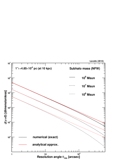
Figure 3: The dimensionless ${\cal J}_{\rm single}$ factors for three different subhalo masses, taken in the range $10^{6}-10^{8}\mbox{$M_{\odot}$}$, as functions of the resolution angle $\theta_{\rm res}$. The analytical approximation proposed in Lavalle et al. (2010) is also shown. All objects are assumed to be located at 10 kpc from the observer. This factor is computed using $\psi=0^{\circ}$, where $\psi$ refers to the angle of the line of sight with the subhalo center.

To study the contribution of isolated objects, we consider three subhalos within the mass range $10^{6}$-$10^{8}$ $M_{\odot}$ and with inner NFW density profiles — adopting instead an Einasto shape would not change the final results. Their radial extents $r_{200}$ are connected to their scale radii $r_{s}$ via the concentration parameter $c_{200}$ through the relation $c_{200}=r_{200}/r_{s}$. The parameters that we use are reported in Table 1, where the angular sizes of the scale radii are given assuming a distance to the observer of 10 kpc for all objects. These parameters are close to those inferred from the Via Lactea II setup used in Pieri et al. (2009), to which we refer the reader for more details, and roughly correspond to what can be expected for subhalos located at $\sim 10$ kpc from the Galactic center (the closer to the Galactic center, the more concentrated).

Subhalo mass	$r_{200}$	$c_{200}$	$r_{s}$	$\rho_{s}$
$[\mbox{$M_{\odot}$}]$	$[{\rm kpc}]$		$[{\rm pc}\,(^{\prime})^{\dagger}]$	$[{\rm GeV/cm^{3}}]$
$10^{6}$	$2.01$	$56.7$	$35.4$ $(12.2^{\prime})$	$22.2$
$10^{7}$	$4.32$	$50.0$	$86.4$ $(29.7^{\prime})$	$15.9$
$10^{8}$	$9.31$	$43.5$	$213.9$ $(73.5^{\prime})$	$11.0$

Table 1: NFW parameters of the subhalos used for the isolated source analysis. ^† The angular size associated with the scale radius $r_{s}$ is derived assuming that the object is located at a distance of 10 kpc from the observer.

From Table 1, we can already notice that, since most of the annihilation should occur within the scale radius of an NFW target, all objects look extended to any (sub)arcmin-resolution experiment when assuming a distance of 10 kpc and a diffusionless transport for electrons. Since the scale radius roughly scales like $M^{1/3}$, the biggest resolved objects have masses $\lesssim 10^{3}\mbox{$M_{\odot}$}$ at this distance. Interestingly enough, the lower mass range down to $10^{-6}\mbox{$M_{\odot}$}$ is the one that dominates the overall subhalo contribution for a pdf mass index larger than 1.9 Lavalle et al. (2008) — it is equal to 2 in the Via Lactea II model adopted here — which itself bypasses the smooth host halo yield. Therefore, treating apart big subhalos as we do here has no consequence on the average subhalo contribution that we worked out earlier, which does not have to be depleted. As we will see later, however, the subhalo size does not reflect, in fact, the actual electron distribution extent associated with the object, due to spatial diffusion effects.

It is clear that though extended, our template single subhalos should increase the detection potential if crossing the line of sight of the telescope, because of the dark matter cusps they contain. To estimate the corresponding optical depths, we can first calculate the ${\cal J}_{\rm single}={\cal J}_{2}(\psi=0^{\circ})$ factor defined in Eq. (14) for each object, which implicitly corresponds to using the diffusionless limit. We show our results in Fig. 3, where ${\cal J}_{\rm single}$ is plotted against the angular resolution. We see that for an angular resolution around 1’, values of $\sim 10^{3}$-$10^{4}$ can be reached for a big subhalo located at a distance of 10 kpc. By using Eqs. (III.2.1) and (16) and parameters therein, this translates into an optical depth of $\langle\tau^{\chi}_{n}\rangle\sim 10^{-5}$-$10^{-4}$. Note that since the angular extent of the scale radii of our objects is larger than the reference angular resolution of 1’, we can use the line-of-sight approximation of ${\cal J}_{2}$ proposed in Ref. Lavalle et al. (2010), which is analytical (denoted ${\cal J}_{\rm los}^{2}$ in their Eq. 3.20). The relation between both formalisms is the following:

$${\cal J}_{2}(\psi=0^{\circ}) \approx \frac{r_{s}}{r_{0}}\,\left[\frac{\rho_{s}}{\rho_{0}}\right]^{2}\,{\cal J}_{\rm los}^{2}$$

$$\approx \left[\frac{\rho_{s}}{\rho_{0}}\right]^{2}\,\frac{(1+\mu_{\rm res})\,\pi}{2}\frac{r_{s}^{2}}{r_{0}\,b_{\rm res}}\;,$$

where $b_{\rm res}\equiv d\,\sin\theta_{\rm res}$ is the impact parameter. This approximation is demonstrated to be very accurate in Fig. 3 except when the angular resolution exceeds the subhalo scale radius. We recall that the main assumption behind this formula is to approximate an inner profile to its central behavior namely $\rho(r)\approx\rho_{s}(r/r_{s})^{-\gamma}$.

Such a result, i.e. $\langle\tau^{\chi}_{n}\rangle\sim 10^{-5}$-$10^{-4}$, might fall within the current experimental sensitivities and is therefore worth being more deeply investigated — note, however, that it is obtained for a quite light WIMP of 1 GeV. In particular, it is important to study the additional and fundamental role of spatial diffusion.

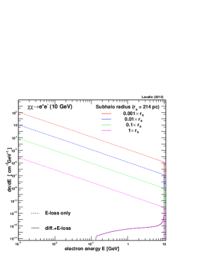
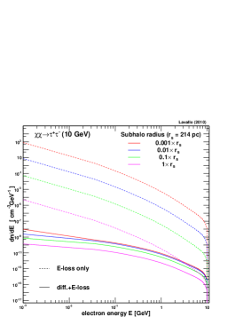
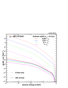
Figure 4: Left: comparison of the electron density obtained in a full diffusion model, at different positions in the $10^{8}\mbox{$M_{\odot}$}$ subhalo of Table 1, with the electron density calculated in the diffusionless approximation; a monochromatic injection of 10 GeV electrons is assumed. Middle (Right): same as left panel, but assuming a $\tau^{+}\tau^{-}$ ($b\bar{b}$) injection spectrum.

III.2.5 A focus on spatial diffusion effects

Our most critical assumption so far was to neglect the spatial diffusion of electrons, so it is first interesting to compare the relevant spatial scales. An angular size of 1’ corresponds to a physical of $\sim 3$ pc for a target located at 10 kpc, scaling almost linearly with the distance. If we write the diffusion coefficient as $K(E)\equiv K_{0}(E/E_{0})^{\delta}$ (see e.g. Berezinskii et al. (1990)), then the electron propagation scale $\lambda$ can be defined in a steady-state regime as

$$\lambda^{2}(E\leftarrow E_{s}) \equiv 4\int_{E}^{E_{s}}dE^{\prime}\frac{K(E^{\prime})}{b(E^{\prime})}$$

$$= 4\,K_{0}\,\tau_{l}\frac{(E_{0}/E)^{1-\delta}}{(1-\delta)}\left[1-\left(\frac{E}{E_{s}}\right)^{1-\delta}\right]\;,$$

where $b(E)$ is the energy-loss rate (taken in the Thomson approximation), $E_{s}$ the injected electron energy and $E<E_{s}$ the energy after the electron has propagated over a distance of $\lambda>0$ on average. It is difficult to determine the diffusion coefficient far away from the Galactic disk because most of observational constraints are local (see e.g. Maurin et al. (2001) or Strong and Moskalenko (1998)). Nevertheless, we can consider the local value as a lower bound, since diffusion is expected to be more efficient in a less dense and less turbulent medium Shalchi (2009) — the densities of interstellar matter and cosmic rays are expected (and observed) to decrease with the distance to the disk. For simplicity, let us assume that $K_{0}=3\times 10^{27}\,{\rm cm^{2}/s}$ ($E_{0}=1$ GeV) and $\delta=0.7$, values close to those inferred from local constraints (see e.g. Maurin et al. (2001); Putze et al. (2010)). Further supposing, as before, that the energy-loss rate is only driven by interactions with the CMB, we have,

$$\lambda(E\leftarrow E_{s}) = 12.6\,{\rm kpc}\,$$

$$\times\left\{\left[\frac{1\,{\rm GeV}}{E}\right]^{0.3}-\left[\frac{1\,{\rm GeV}}{E_{S}}\right]^{0.3}\right\}^{1/2}\;.$$

Thus, if we consider an injected energy of $E_{s}=1$ GeV, the propagation scale becomes larger than $\sim 3$ pc for $\delta E\equiv E_{s}-E>2\times 10^{-7}$ GeV. This tremendously small value of $\delta E$ actually defines the spectral domain of validity of our previous estimate of the optical depth, when spatial diffusion was neglected. The actual electron density traces the squared dark matter density in subhalos at the very moment of injection, and is smeared out afterwards due to propagation effects, which induces the formation of a core of electrons. By comparing the scales, it is clear that diffusion effects completely overcome angular resolution effects: the propagation scale derived above is as large as, or even larger than, a big subhalo itself. The fact that the smearing due to propagation dominates angular resolution effects was already emphasized in the context of galaxy clusters in Ref. Lavalle et al. (2010), and in the context of dwarf spheroidal galaxies in Refs. Colafrancesco et al. (2007); Huang et al. (2010). More generally, smearing effects are important whenever the source gradient is large over a typical diffusion length.

To more precisely illustrate the role of spatial diffusion, we adopt a very simple three-dimensional isotropic and homogeneous diffusion model which is defined by the steady-state equation

$$-K(E)\,\Delta{\cal N}(E,\vec{x})-\partial_{E}\left\{b(E)\,{\cal N}(E,\vec{x})\right\}={\cal Q}(E,\vec{x})\;,$$

for which the Green function is analytical:

$${\cal G}(E,\vec{x}\leftarrow E_{s},\vec{x}_{s})=\frac{\exp\left\{-\frac{\left(\vec{x}-\vec{x}_{s}\right)^{2}}{\lambda^{2}}\right\}}{b(E)\left[\pi\,\lambda^{2}\right]^{3/2}}\;.$$ (23)

Supposing a still subhalo, the propagated equilibrium electron density at position $\vec{x}$ in the subhalo is therefore given by plugging the previous Green function into Eq. (4).

In Fig. 4, we report the equilibrium electron density calculated for different positions in the $10^{8}\mbox{$M_{\odot}$}$ subhalo featured in Table 1, obtained both (i) in the diffusionless approximation (dashed curves) and (ii) in a full diffusion-loss propagation model (solid curves). A direct annihilation into electron-positron pairs is assumed in the left panel ($E_{s}=\mbox{$m_{\chi}$}$), and for completeness, we also consider the case of a $\tau^{+}\tau^{-}$ ($b\bar{b}$) annihilation spectrum in the middle (right) panel. For each case, we take a WIMP mass of 10 GeV and the canonical value for the annihilation cross section, and we compute the electron density at different positions in the subhalo in between a thousandth of $r_{s}$ and $r_{s}$, i.e. in the bulk of the injection region. We stress that a 10 GeV WIMP annihilating into $b\bar{b}$ pairs is already likely excluded by cosmic-ray antiproton data Lavalle (2010), but such an example is still useful in terms of spectral properties. In the left panel, the diffusionless approximation is demonstrated to tend towards the full calculation only in the limit $\delta E\rightarrow 0$, as expected, while the discrepancy is shown dramatic over the remaining — i.e. almost entire — part of the spectrum. We notably see that below $\sim 200$ MeV, all electrons have diffused away from the subhalo, and that their density is almost constant all over it for higher energies — except for $\delta E\rightarrow 0$. This can be understood from Eq. (III.2.5): for $E_{s}=10$ GeV, $\lambda$ becomes larger than $r_{s}=214$ pc when $\delta E\gtrsim 0.1$ GeV, which results into smearing the differential electron density over that scale, setting a cored spatial distribution over most of the spectrum. In this pair-injection case, the diffusionless approximation can lead to an overestimate of the electron density by more than 3 orders of magnitude, a discrepancy that strongly increases from the edge of $r_{s}$ to the very central region of the subhalo. The error is slightly decreased when considering a continuous $\tau^{+}\tau^{-}$ or $b\bar{b}$ spectrum because injection proceeds at any energy less than the WIMP mass. In that case, it still amounts to a few orders of magnitude, increasing when energy decreases. We also note that though the annihilation rate varies by a factor of $\sim 4,000^{2}$ (NFW case) between $r_{s}$ and $0.001\,r_{s}$, the differential electron density only spans a bit less than 2 orders of magnitude in the $\tau^{+}\tau^{-}$ or $b\bar{b}$ case, which shows that diffusion is a very efficient spatial smearing process. It is therefore clear that accounting for spatial diffusion will rescale the optical depth to much lower values than estimated before in the case of individual massive subhalos.

In Fig. 4, we have assumed $K_{0}=3\times 10^{27}\,{\rm cm^{2}/s}$ for spatial diffusion. Such a value, which is constrained locally, is not expected to be relevant to regions distant by more than a few kpc from the Galactic plane, where diffusion should become closer and closer to free propagation. Nevertheless, we emphasize that using a more realistic value will not qualitatively change our argument about spatial diffusion. Indeed, a more realistic value for the $K_{0}$, though still to be determined, should at least be larger than the local one, and would therefore lead to a larger propagation scale for electrons, which even strengthens the diffusion effect.

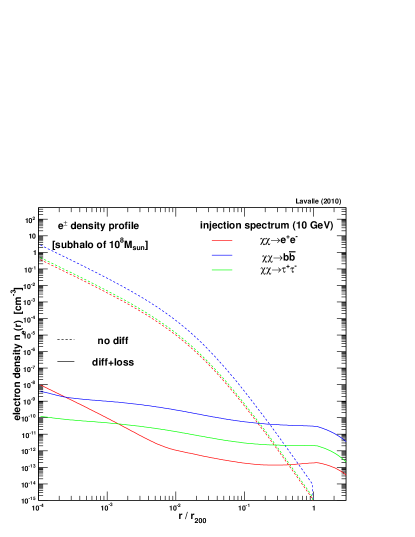
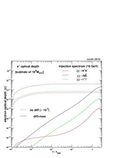
Figure 5: Left: Electron density as a function of the subhalo radius for different injection spectra. Right: Corresponding optical depth against the subhalo radius ($r=l/2$, where $l$ is the line-of-sight length). In both panels an annihilating 10 GeV WIMP is assumed; dashed curves represent the diffusionless case, while solid curves refer to a full diffusion-loss transport model.

We can now go further in the calculation of the optical depth by adopting the full diffusion-loss transport model described above. In Fig. 5, we derive the electron density profile associated with our $10^{8}$ subhalo (left panel) and the corresponding cumulative optical depth (right panel). We again consider a 10 GeV WIMP annihilating into the three different final states discussed above and illustrate the discrepancy between a full diffusion-loss transport model (solid curves) and the diffusionless approximation (dashed curves). In the left panel, the electron density as derived in the full transport model exhibits a quasicore up to the subhalo extent $r_{200}=9.3$ kpc, which is incidentally of the same order of $\lambda$, whereas the diffusionless density scales completely differently like $\rho^{2}(r)\propto r^{-2}$ — in the full transport model, the electron profile extends beyond the subhalo itself. This has important consequences for the optical depth (right panel), which is the line-of-sight integral of the density, since it increases linearly with the radius up to $r_{200}$ in the former case, while logarithmically in the latter case. The total optical depth can be read off at the border of the object, and we see that the discrepancy between the two transport hypotheses lies within 3 to 5 orders of magnitude, from soft to hard spectral properties (the diffusionless curves are rescaled by a factor of $10^{-3}$). Finally, we see that for such a massive subhalo and for a 10 GeV WIMP with canonical properties, the optical depth $\tau_{e}<10^{-11}$, far away from experimental sensitivities. Going to lower WIMP masses would favor the annihilation into lepton-antilepton pairs and would therefore not benefit of the favorable $1/\mbox{$m_{\chi}$}^{2}$ factor as optimally as necessary.

To summarize this section, we find that, considering the GeV mass scale for WIMPs, subhalos are not expected to provide an observable SZ contribution due to the very weak optical depth they generate — of the order of $\tau_{e}\lesssim 10^{-9}$ collectively down to $\tau_{e}\lesssim 10^{-11}$ individually, for a 10 GeV annihilating particle. In the former case, our calculations were derived in the optimistic diffusionless limit but still led to pessimistic values. In the latter case, spatial diffusion was shown to have the most dramatic impact on predictions because it dilutes away the electron density injected at high rate at subhalo centers. This is in agreement with the pessimistic results found in the context of dwarf spheroidal galaxies Colafrancesco et al. (2007); Huang et al. (2010), which can be considered as very massive subhalos, though with a sizable baryon fraction inside — the energy-loss rate of electrons is then driven by ionization at low energy. For annihilating dark matter, decreasing the WIMP mass down to the MeV scale would increase the electron injection rate by 6 orders of magnitude if one merely considers the favorable $1/\mbox{$m_{\chi}$}^{2}$ scaling relation. Nevertheless, we see from the right panel of Fig. 5 that this would even not be sufficient to get a reachable optical depth, since the annihilation channel would be $e^{+}e^{-}$ in that case. Moreover, other astrophysical constraints on the annihilation cross section, from x-rays or gamma rays, must then also be taken into account, which can be summarized as $\mbox{$\langle\sigma v\rangle$}\lesssim 10^{-31}\,{\rm cm^{3}/s}\,(\mbox{$m_{\chi}$}/{\rm MeV})^{2}$ Boehm et al. (2004); Ascasibar et al. (2006). Such constraints strongly limit the possible increase in the optical depth. Other ways to increase the electron density can still be advocated, like the presence of black holes in the centers of some subhalos. We discuss this hypothesis in the next section.

IV Additional impacts from intermediate-mass black holes

In this section, we complete the study of Galactic dark sources by considering a putative population of IMBHs.

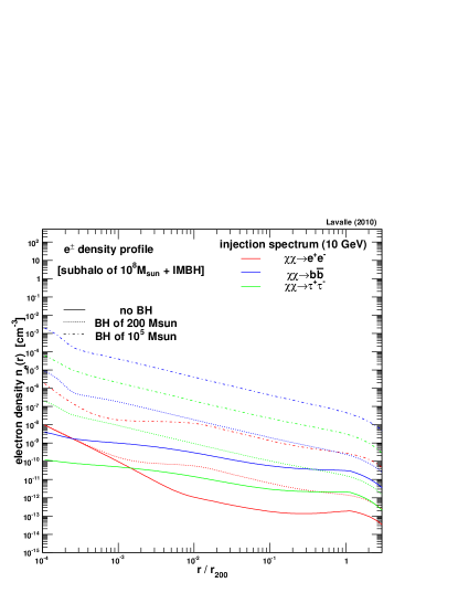
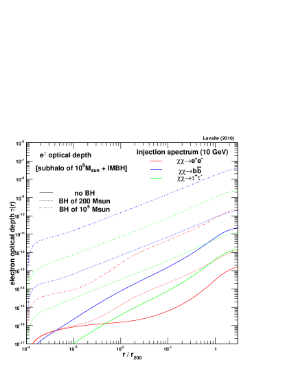
Figure 6: Same as Fig. 5, except that the solid curves characterize a subhalo without IMBH, the dotted curves the same subhalo hosting a $200\mbox{$M_{\odot}$}$ IMBH, and the dash-dotted curves the same subhalo hosting a $10^{5}\mbox{$M_{\odot}$}$ IMBH.

BH mass	$r_{h}$	$r_{\rm sp}$	$\rho_{\rm sp}$	$r_{\rm sat}$	$r_{\rm sch}$
$[\mbox{$M_{\odot}$}]$	$[{\rm pc}]$	$[{\rm pc}]$	$[10^{4}\,{\rm GeV/cm^{3}}]$	$[10^{-3}\,{\rm pc}]$	$[10^{-11}\,{\rm pc}]$
$200$	$1.02$	$0.20$	$114.81$	$4.17$	$1.92$
$10^{5}$	$24.41$	$4.88$	$4.59$	$25.17$	$960$

Table 2: Spiky-NFW parameters for a prototype $10^{8}$ $M_{\odot}$ subhalo hosting a black hole of (i) 200 and (ii) $10^{5}$ $M_{\odot}$. The remaining subhalo parameters can be found in Table 1.

Although the formation scenario of IMBHs is still debated and probably not unique, there are many observational hints for their existence, as e.g. ultra-luminous x-ray sources (see Farrell et al. (2009) for a recent case, and Miller and Colbert (2004) for a review). Among interesting possibilities, IMBHs could be the end products of very massive Population III stars, those with typical masses $\gtrsim 250\,\mbox{$M_{\odot}$}$ Bond et al. (1984), and thereby seed the supermassive black holes observed in most of the galaxies Madau and Rees (2001).

If IMBHs are common objects among the first stars, some should still wander in the halos of galaxies. One appealing idea is that if they have formed from baryon gas cooling in protohalos of dark matter, they could have raised minispikes from the adiabatic compression of the surrounding dark matter Gondolo and Silk (1999), making them excellent Galactic or extragalactic targets in the search for dark matter annihilation signals. This idea was proposed in Ref. Zhao and Silk (2005) for gamma-ray searches, and further promoted with more details in Ref. Bertone et al. (2005) (see also Fornasa and Bertone (2008) for a recent review). The authors of the latest reference discussed scenarios in which the number of Galactic IMBHs — within a Galactic radius of $\sim 200$ kpc — could vary from hundreds to thousands.

The most optimistic scenarios are already in tension with current observations in gamma-ray astronomy Bringmann et al. (2009), but the general picture is still valid and can be probed with new generation large-field-of-view gamma-ray instruments, like the Fermi satellite Taoso et al. (2009). For a better relevance in the frame of dark matter searches, it is important to detect such signals outside the Galactic disk and bulge to escape astrophysical foregrounds and minimize interpretation issues. Likewise, it is important to detect complementary signatures which could help to confirm or infirm their dark matter origin. Antimatter cosmic rays are probably not interesting (i) because the astrophysical background is not under control in some cases, (ii) current measurements are compatible with astrophysical explanations (see e.g. Delahaye et al. (2010) for the Galactic electrons and positrons, and Donato et al. (2009) for antiprotons) and (iii) sources distant by more than a few kpc from the Galactic disk are not expected to contribute significantly to the local cosmic-ray flux because of the diffusive nature of their propagation in the interstellar medium. As for subhalos, we check here whether dark matter annihilation around IMBHs could generate any observable SZ signal.

Although some population modelings are available in Bertone et al. (2005), the associated theoretical uncertainties remain to be investigated (see Sandick et al. (2010) for more details on uncertainties). Therefore, it seems safer to concentrate the present analysis on individual objects without accounting for any putative statistical property. Proceeding so, we aim at checking whether isolated high-latitude IMBHs could generate significant SZ contributions in contrast to isolated subhalos. Nonetheless, before starting, it is interesting to use the averaged properties of some minispike scenarios to check their potential as SZ targets. If we take an average annihilation volume $\langle\xi_{\rm sp}\rangle\sim 10^{4}\,{\rm kpc^{3}}$ for minispikes, reminiscent of the most optimistic scenario of Bertone et al. (2005) (see e.g. Brun et al. (2007); Bringmann et al. (2009)), then the total average annihilation rate in those objects is $\propto{\cal S}_{2}\langle\xi_{\rm sp}\rangle$. Converting this in terms of an average electron density inside a $10^{7}\mbox{$M_{\odot}$}$ subhalo of scale radius $r_{s}\sim 100$ pc (annihilation to electron-positron pairs), we get the following zeroth order estimate of the optical depth:

$$\langle\tau^{\chi}_{2}\rangle_{\rm sp} \sim 2\,\sigma_{T}\,{\cal S}_{2}\,r_{s}\,\frac{\langle\xi_{\rm sp}\rangle}{V_{s}}$$

$$\sim 1.95\times 10^{-6}$$

$$\times \frac{{\cal S}_{2}}{1.35\times 10^{-29}\,{\rm cm^{-3}s^{-1}}}\,\frac{\langle\xi_{\rm sp}\rangle}{10^{4}\,{\rm kpc^{3}}}\,\left[\frac{r_{s}}{100\,{\rm pc}}\right]^{-2}\;,$$

where ${\cal S}_{2}$ was computed using $\mbox{$m_{\chi}$}=10$ GeV with the other canonical values, and where we have assumed that $r_{0}\,{\cal J}_{2}\sim r_{s}\,\langle\xi_{\rm sp}\rangle/V_{s}$. This is thereby worth a more detailed investigation.

Aside from statistical properties that may depend on structure formation and evolution, considering single IMBHs allows us to motivate a quite generic modeling of dark matter distribution around them by simply accounting for the adiabatic compression Gondolo and Silk (1999) of the host dark matter microhalo during the IMBH growth — this is also one of the main assumptions of Ref. Bertone et al. (2005), upon which the authors plugged an evolution history by means of numerical simulations to estimate the survival population statistical properties. Thus, starting from a microhalo density profile scaling like $r^{-\gamma}$, the adiabatic growth of a forming IMBH raises a spike of index $\gamma_{\rm sp}=(9-2\gamma)/(4-\gamma)$ by angular momentum conservation. For instance, choosing $\gamma=1$ (NFW) implies a spike index of $\gamma_{\rm sp}=7/3\simeq 2$. Further adopting an NFW initial profile as a generic case, the final dark matter density shape around the IMBH can be described as

$$\rho(r)=\begin{cases}\rho_{\rm sat}\;\;\;\;&r_{\rm sch}<r\leq r_{\rm sat}\\ \rho_{\rm sp}\left(\frac{r}{r_{\rm sp}}\right)^{-\gamma_{\rm sp}}&r_{\rm sat}<r\leq r_{\rm sp}\\ \rho_{s}\frac{(r/r_{s})^{-1}}{(1+r/r_{s})^{2}}&r>r_{\rm sp}\end{cases}$$ (25)

where the subscript sp is related to the spike (density, extent, index), $r_{\rm sat}$ is the radius at which the annihilation rate saturates  Berezinsky et al. (1992), and $r_{\rm sch}=2\,G\,m_{\rm bh}/c^{2}\simeq 9.6\times 10^{-14}{\rm pc}\,(m_{\rm bh}/\mbox{$M_{\odot}$})$ is the Schwarzschild radius of a black hole of mass $m_{\rm bh}$ below which neither particles nor light can get out Schwarzschild (1916). We have the implicit relation $\rho_{\rm sp}\simeq\rho_{s}\,r_{s}/r_{\rm sp}$, provided $r_{\rm sp}\ll r_{s}$. The actual spatial scales can be inferred from the radius of gravitational influence $r_{h}$ of the black hole. It was indeed found in Ref. Bertone et al. (2005) that $r_{\rm sp}\approx 0.2\,r_{h}$ in most cases. Furthermore, it turns out that $r_{h}$ can be related to $r_{s}$ from the implicit equation  Merritt (2004, 2006),

$$M(<r_{h})=4\,\pi\int_{0}^{r_{h}}dr\,r^{2}\,\rho(r)=2\,m_{\rm bh}\;,$$ (26)

which is analytical in the NFW case:

$$\frac{2\,m_{\rm bh}}{4\,\pi} = \rho_{s}\,r_{s}^{3}\left[\ln\left\{\frac{r_{h}+r_{s}}{r_{s}}\right\}-\frac{r_{h}}{r_{h}+r_{s}}\right]$$ (27)

$$\approx \frac{\rho_{s}\,r_{s}\,r_{h}^{2}}{2}\;.$$ (28)

The last line was obtained with the limit $r_{h}\ll r_{s}$, eventually leading to

$$r_{h} \approx \sqrt{\frac{\,m_{\rm bh}}{\pi\,\rho_{s}\,r_{s}}}$$

$$\approx 3.9\,{\rm pc}\,\left[\frac{m_{\rm bh}}{100\,\mbox{$M_{\odot}$}}\left[\frac{\rho_{s}}{10\,{\rm GeV/cm^{3}}}\frac{r_{s}}{100\,{\rm pc}}\right]^{-1}\right]^{1/2}\;.$$

Note that this approximation is only valid for $r_{h}\ll r_{s}$; Eq. (27) must be used otherwise. Now, although the spike radius should in principle be computed numerically, we can use the scaling relation $r_{\rm sp}\approx 0.2\,r_{h}$ Merritt (2004). Finally, all these spatial scales have to be compared with the saturation radius defined by the saturation density Berezinsky et al. (1992),

$$\rho_{\rm sat}\equiv\rho(r_{\rm sat}) \approx \frac{\mbox{$m_{\chi}$}}{\mbox{$\langle\sigma v\rangle$}t_{\rm bh}}$$

$$\approx 10^{8}\,{\rm GeV/cm^{3}}$$

$$\times\,\frac{\mbox{$m_{\chi}$}}{\rm GeV}\left[\frac{\mbox{$\langle\sigma v\rangle$}}{3\times 10^{-26}{\rm cm^{3}/s}}\frac{t_{\rm bh}}{10\,{\rm Gyr}}\right]^{-1}\;,$$

where $t_{\rm bh}$ is the black-hole age.

We now take a template example relying on the study of single subhalos we performed in Sec. III.2.5, implying quite a massive subhalo of $10^{8}\mbox{$M_{\odot}$}$, the NFW profile of which has now to be compressed and develop a spike because of the presence of an IMBH in its center. We consider two IMBH mass cases reminiscent of the scenarios proposed in Bertone et al. (2005), a soft case with $m_{\rm bh}=200$ $M_{\odot}$ and a strong case with $m_{\rm bh}=10^{5}$ $M_{\odot}$(see also Fornasa and Bertone (2008)). The associated parameters that we derived according to Eqs. (26-IV) are listed in Table 2. We are thus armed to calculate the electron density arising from dark matter annihilation in such objects, using the same diffusion-loss transport model as in Sec. III.2.5.

We plot our results in Fig. 6, where the electron density profile is reported in the left panel and the corresponding cumulative optical depth appears in the right panel. We compare three different configurations: a single $10^{8}$ $M_{\odot}$ subhalo (solid curves, same as in Fig. 5), the same subhalo with a $200$ $M_{\odot}$ central black hole (dotted curves), and with a $10^{5}$ $M_{\odot}$ central black hole (dash-dotted curves). As before, we assumed a 10 GeV WIMP with the annihilation channels discussed above. As expected, we see that the presence of a central black hole (through its related spike) has drastic consequences on predictions. The optical depth is shown to increase by 1 (3) order of magnitude provided a spike raised by a $200$ ($10^{5}$) $M_{\odot}$ central black hole, independently of the injection spectrum. This can actually be related to the increase of the annihilation rate averaged over the diffusion length, which, unfortunately, has no analytical form. The optical depth can reach $\tau_{e}\sim 10^{-7}$ in the most favorable $b\bar{b}$ spectral case, but such a level is still, unfortunately, irrelevant to observation.

V Conclusion

In this paper, we have studied the SZ effect potentially generated by dark matter annihilation (or decay) products on the Galactic scale, in the high-latitude sky. We have focused our analysis on (i) the smooth Galactic halo (see Sec. III.2.1), (ii) subhalos (see Sec. III.2.2) and (iii) putative spikes raised by black holes in the centers of individual subhalos (see Sec. IV). We have considered canonical properties for annihilating (or decaying) dark matter, though in the very light mass range below 10 GeV.

For the smooth-halo contribution, we have derived our predictions in the diffusionless limit of the electron transport, which is valid whenever the electron injection rate does not vary significantly over a diffusion length. In this approximation, we have found that $\tau_{e}\lesssim 10^{-8}$ for a 1 GeV annihilating or decaying WIMP, rescaled to $\lesssim 10^{-10}$ for a 10 GeV annihilating WIMP. The average contribution of subhalos was then shown to boost the signal by 1 order of magnitude at most in the case of dark matter annihilation, but only when using a rather favorable subhalo phase space (mass index of 2) — the effect is strongly diminished for decaying dark matter, since the injection rate then scales like the density, not like the squared density; we did not further explore the impact of subhalos in this context.

The study that we performed on isolated subhalos has led us to abandon the diffusionless limit of electron transport, which was shown unjustified for a source exhibiting a strong spatial gradient over the typical diffusion length (like the central cusps of galaxy clusters Lavalle et al. (2010)). Indeed, a $10^{8}$ $M_{\odot}$ subhalo, i.e. quite massive, has a radial extent of a few kpc, of the same order as the diffusion length. We have notably illustrated how a core radius emerges in the electron distribution because of spatial diffusion, independently of injection spectra. This smearing strongly dilutes the electron density so that the optical depth cannot reach values of interest. For a quite massive subhalo of $10^{8}$ $M_{\odot}$, we found an optical depth $\tau_{e}\lesssim 10^{-11}$ for a 10 GeV annihilating WIMP with canonical properties. These results are in agreement with those obtained in similar studies on dwarf spheroidal galaxies Colafrancesco et al. (2007); Huang et al. (2010).

Finally, we checked whether dark matter spikes raised by IMBHs in massive subhalos from adiabatic compression could lead to observable SZ signals. To proceed, we have designed a generic spike modeling featured by the properties of the host subhalo and by the IMBH mass. We have focused on a template example consisting in a 200 ($10^{5}$) $M_{\odot}$ central black hole located at the center of a $10^{8}$ $M_{\odot}$ subhalo. We have shown that such a spike could boost the optical depth by 1 (3, respectively) order of magnitude, which is in fact related to the increase in the annihilation rate averaged over a typical diffusion length. Nevertheless, even such an increase is not enough to get an electron density large enough for leaving a SZ imprint in the CMB sky. We found $\tau_{e}\lesssim 10^{-7}$ for our 10 GeV WIMP, which leads us to conclude that dark matter is globally not expected to generate SZ fluctuations on the Galactic scale. Because of these quite modest values obtained for the optical depth, it is not necessary to go deeper in the spectral analysis to derive the full SZ distortion spectrum Lavalle et al. (2010).

Note that when dealing with isolated massive subhalos, hosting IMBHs or not, we have computed the electron densities in the frame of a diffusion-loss transport model for which we assumed a local diffusion coefficient and an energy loss driven by interactions with CMB only. Though the latter hypothesis seems reasonable far away from the Galactic disk in a medium almost devoid of gas and stars, the former is more difficult to justify, since electrons should be close to free propagation in such regions. Nevertheless, we have argued that considering a more realistic transport would actually strengthen the advocated smearing effect coming from spatial diffusion, since the diffusion coefficient should then be increased, which in fact makes our predictions rather conservative. Still, more accurately relating the phenomenology of transport to the interstellar medium properties remains a vast topic to undertake so as to improve all analyses focused on nonthermal cosmic-ray electron-induced radiations.