Adaptive selective sidelobe canceller beamformer with applications in radio astronomy
Abstract
We propose a new algorithm, for parameter estimation that is applicable to imaging using moving and synthetic aperture arrays. The new method results in higher resolution and more accurate estimation than commonly used methods when strong interfering sources are present inside and outside the field of view (terrestrial interference, confusing sources).
I Introduction
When multiple antennas or other sensors are used to estimate incoming signals, it is best to treat them all as a single array and apply one of the known array processing algorithms for the estimation. In various situations, however, this is not practical or even impossible.
In radio-astronomy, the antenna array moves with the rotation of the Earth. Correlations between the antenna can be obtained for a given time, but not between different points in time. Denote by the measured correlation matrix (visibility) of the array at time ; the combined correlation matrix of epochs can be written as
| (1) |
where some of the matrix elements are unknown. The matrices need not be of the same size.
The need to overcome this obstacle is as old as the days of radio astronomy itself. The standard approach to process the measured correlations (a.k.a visibility) is through using inversion (see [1] page 128 and [2])
| (2) |
where are the baselines (i.e., distances between the antennas at the measurement time), is the number of measurements and is the estimated power: in other words, dirty image. This is optimal as long as epochs are independent. However, sidelobes of interfering sources are not spatially white, thus making this approach sub-optimal. The dirty image is used for further processing, by deconvolution algorithms to yield a better image.
The most widely used deconvolution algorithm is the CLEAN (proposed by Högbom [3]) and its many variants. The CLEAN algorithm assumes that the observed field of view is composed of point sources. CLEAN iteratively removes the brightest point source from the image until the residual image is noise-like. The point sources are accumulated during the iteration and the reconstructed image is the accumulated source list convolved with a reconstruction beam (usually a Gaussian). During the iterations, CLEAN subtracts the strongest point sources either in the image domain or in the visibility domain. The visibility domain CLEAN is more accurate since we are not limited to pixel resolution. Throughout this paper, we use the visibility domain CLEAN. Acceleration of the CLEAN algorithm can be achieved by estimating multiple point sources based on a single dirty image (major cycle), as well as defining windows for the search procedure. Practically, defining windows reduces the size of the search space. A multi scale CLEAN proposed by Cornwell [4] models the brightness of the sky by the sum of the components of the emission having different size scales. Extensions of the CLEAN algorithm to support wavelets as well as non co-planar arrays are reviewed by Rau et al. in [5].
A matrix based imaging technique which proved equivalence between the radio astronomical problem and the signal processing formulation using beamforming was proposed by Leshem and van der Veen [6] and further analyzed by Ben-David and Leshem [7]. Using the matrix based technique, Leshem and van der Veen [8] suggested a method for the cancellation of strong interference from a small number of interfering sources.
I-A Matrix Based Imaging
In this section we show the equivalence of the standard approach to dirty image calculation and classic (i.e., Bartlett) beamforming (see [9], [10] and [7] for an in depth discussion). In this section we assume a calibrated array (extension for calibration is not hard).
At the ’th epoch, the measured correlation matrix is given by
| (3) |
where is the correlation (visibility) between antenna and antenna located at baseline on the ’th epoch. The array steering vector is defined by
| (4) |
where is the location of antenna at the ’th epoch, relative to some convenient point , are the direction cosines , is the number of antennas in the array and is the wavelength. For epochs, we have and from Equation (2)-(4) we obtain that the relation between the dirty image and the measured correlation matrices is given by
| (5) |
which is the classic (Bartlett) beamformer with weight vector .
In the general case, for a weight vector , the dirty image is given by
| (6) |
I-B MVDR Beamformer
The MVDR (Minimum Variance Distortionless Response) beam-former is designed for scenarios that include interfering sources in the field of view. Its weights are set to minimize the influence of the interfering sources while passing signals from the desired direction (i.e., to minimize the interfering power entering the array via its ‘sidelobes’).
The MVDR is also designed to obey the distortionless response condition; in the absence of noise, the array input and output signals should be equal. Thus,
| (7) |
The MVDR beamformer minimizes the total array output power. For a given observed source and thermal noise, the power from interfering sources is minimized. The MVDR weights are determined by solving the following problem:
| (8) |
The solution to Equation (8) is given by
| (9) |
The MVDR is an adaptive method. The weights are determined by the measured visibility. This is unlike the classical beamformer that determines the weights according to the observing angle independent of other radiating sources.
II Adaptive Selective Sidelobe Canceller Beamforming
In this section we present a novel image formation technique. We begin with a simple example that demonstrates the main idea behind the adaptive-selective-sidelobe-canceller (ASSC) algorithm; for a specific observation direction, the received interference through the sidelobes varies strongly as the array rotates.
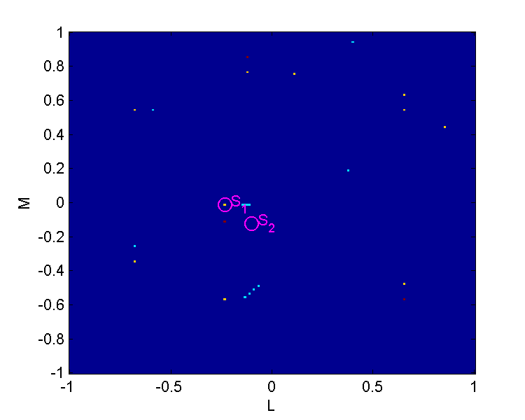
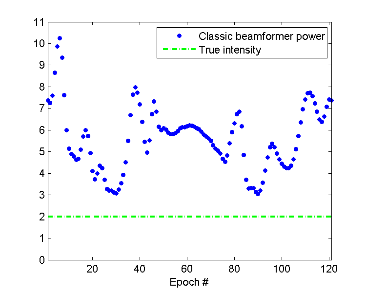
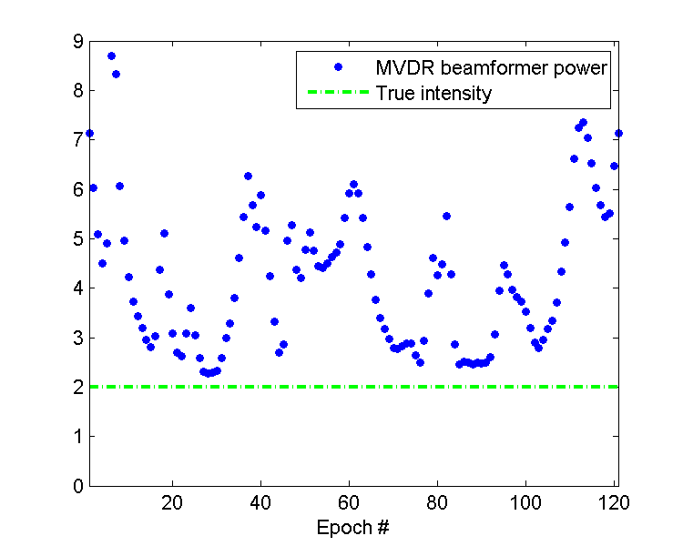
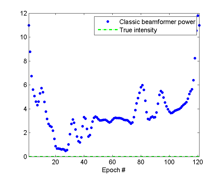
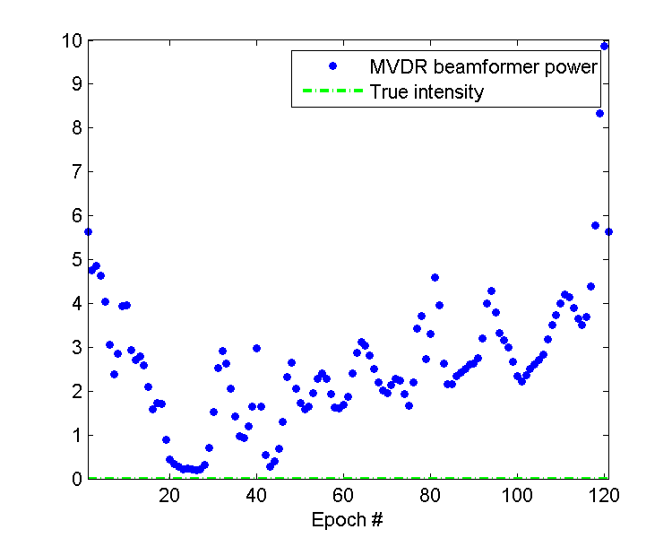
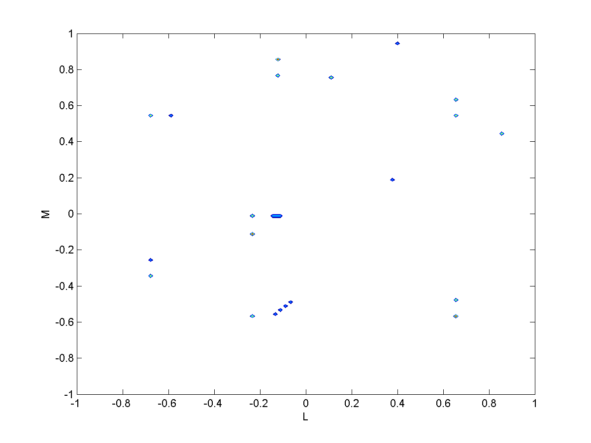
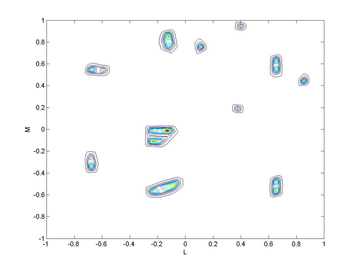
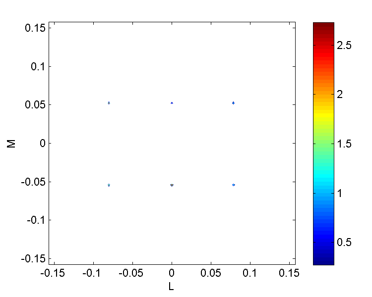
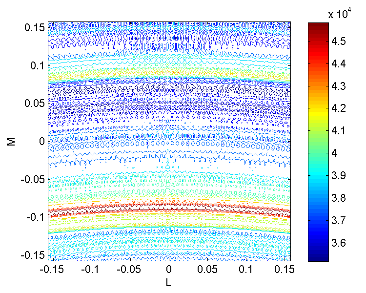
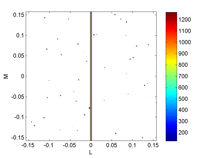
For simplicity, consider an East-West linear array with antennas, spaced, measuring the correlations every minutes for a 12-hour period. The measured correlation matrix at the ’th epoch is . For a specific direction , the output of the ’th beamformer, is composed of the signal-of-interest (SOI) contribution, interfering sources and the noise contribution. The contribution of the interfering sources is determined by their location (and strength) relative to the array sidelobes. Consider a scenario with a few clusters of sources (see Figure (1a)). Figure (1b) shows the output power of the ’th classic beamformer for a direction of a point source (marked at Figure (1a)). Figure (1c) shows the ’th MVDR beamformer for the same direction. From all available time epochs, only a few epochs yield an estimation close to the true point source intensity. The intensity estimation of most epochs is biased due to the interference (received through their sidelobes). The output power of the two beamformers (classic and MVDR) towards the empty direction (marked at Figure (1a)), is plotted in Figures (1d) and (1e) respectively. Only a few time epochs yield a close to zero intensity estimation (the true intensity); whereas most of the epochs estimate biased intensity originated from the interference signal received through their sidelobes. The time epoch with the minimal power for a specific direction yields the best estimator. Averaging the output power for all epochs will result in a biased and inaccurate estimator.
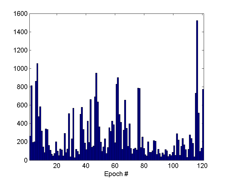
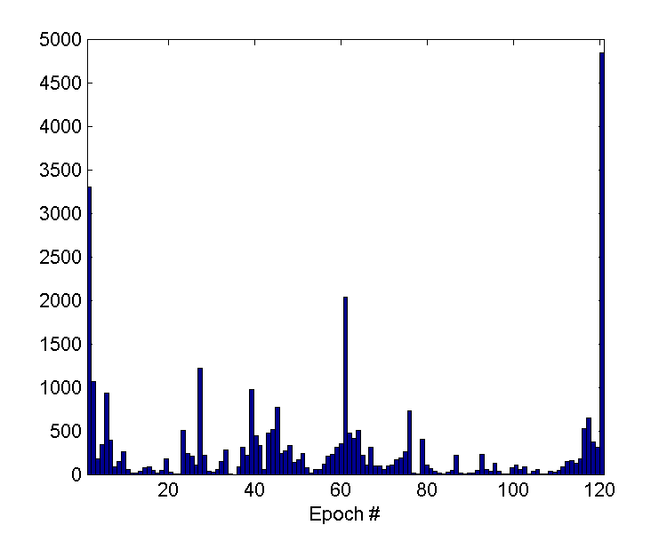
Note that although the number of reliable estimates per direction is small, the total number of correlation matrices for the entire FOV is much larger (it depends on the interference location and the array geometry). Figure (2) shows histograms of the number of directions (pixels) for which a specific correlation matrix estimated the minimal power (i.e., underwent the smallest interference). Simulation conditions are the same as in Figure (1). For the classic beamformer (Figure 2a), out of the pixels in the image, most time epochs (more than ) performed best (i.e.,had minimal interference) for at least pixels. Over of the time epochs benefited from minimal interference for of the pixels in the image. As for the MVDR beamformer, of the available time epochs, most time epochs (more than ) performed best (i.e., had minimal interference) for at least pixels out of the pixels in the image. Over of the time epochs experienced minimal interference for of the pixels in the image.
This example demonstrates that the received array power of a specific observation direction, varies significantly with the array orientation due to interfering sources. Some of the array orientations yield a reliable intensity estimation, whereas others yield a biased intensity estimation (aggravated by the interfering signals).
II-A The ASSC algorithm
Based on the observations above, we now propose an algorithm that exhibits high performance in the presence of interfering sources and images with a high dynamic range. For a given set of correlation matrices, , measured at time epochs (or by different arrays):
-
1.
Calculate the array output power (i.e., dirty image) for each epoch separately according to the desired beamformer,
(10) is the MVDR weight vector given by
(11) -
2.
Determine the ASSC parameters and where is the number of best epochs to consider for each and are their weights. These parameters are best determined using the measured data by plotting a histogram of the calculated for a specific . is determined so no epoch that suffers from significant sidelobes (i.e., has significantly larger power than the minimal power) will be selected. Typically depending on the array geometry and the interference strength and location. As a rule of thumb, the stronger the interference, the smaller the .As for , is should be chosen such that .
-
3.
For each (each pixel in the image) find the best (i.e., smallest) values among all measurements,
(12) where are the smallest elements in the order statistics of
-
4.
Calculate the ASSC power (dirty image) according to
(13)
Similarly, the weight vector from Equation (11) can be chosen using any other beamforming technique (for example classic, AAR). Table (I) summarizes the ASSC beamformer algorithm.
| For each incident angle : |
| Calculate the desired beamformer weight vector for each epoch. |
| Calculate the beamformer output power of each correlation matrix separately, |
| Select the best (i.e., smallest) measurements among |
| Calculate the ASSC dirty image by |
The computational complexity of the ASSC classic/MVDR beamformer is similar to classic/MVDR beamformers respectively, with the following minor addition: for each pixel, find the minimal powers from .
II-B Rationale for the ASSC
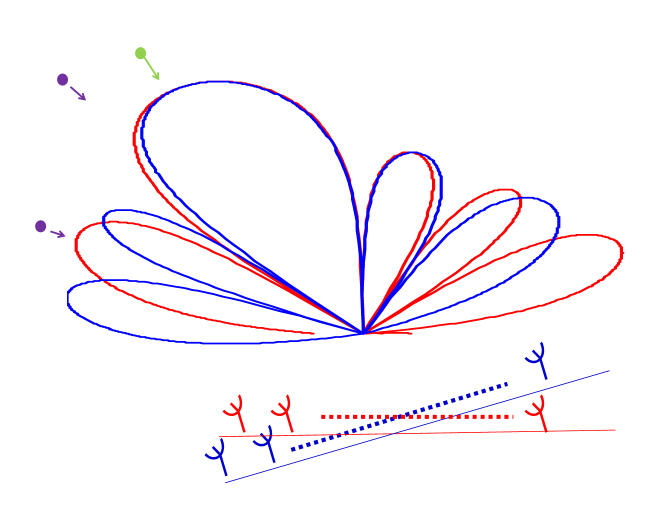
Figure 3 illustrates the sidelobes of a rotating array in two orientations, observing the same SOI (marked in green) in the presence of two interfering sources (marked in purple). The array at the first orientation (marked in red), has a strong sidelobe in the direction of the interfering sources and therefore receives strong interfering power. The array at the second orientation (marked in blue), receives much lower interference power due to the shape and location of its sidelobes relative to the interfering sources. The received power from the interfering sources depends strongly on the direction of the interfering sources relative to the array sidelobes whereas the received power from the SOI is similar for all orientations.
The ASSC method is based on the following observations:
-
a)
If a signal source is present, and noise at the antenna is neglected, all correlation matrices estimate the same incoming signal and its power.
-
b)
The different results, for different time epochs, are due to interfering signals arriving from other directions through the array sidelobes.
-
c)
By choosing the time epoch with the minimal power, we choose the correlation matrix with the smallest interfering power, which happens to best suppress the interference.
Some comments are in place:
-
a)
The proposed method is adaptive and the selected epochs are based on the signal estimates. We implicitly assume that at least one of the array estimations is close to the correct value. If the conditions are such that none of the epochs produce an acceptable estimation, the traditional approaches of averaging may produce more robust results.
-
b)
In the case where the thermal noise at the antenna is significant and averaging over several measurements is needed, the averaging can be performed on a subset of the epochs with the smallest power.
-
c)
It should be noted that this technique can be applied to any kind of array beamforming algorithm.
III Simulation results
III-A In FOV interference
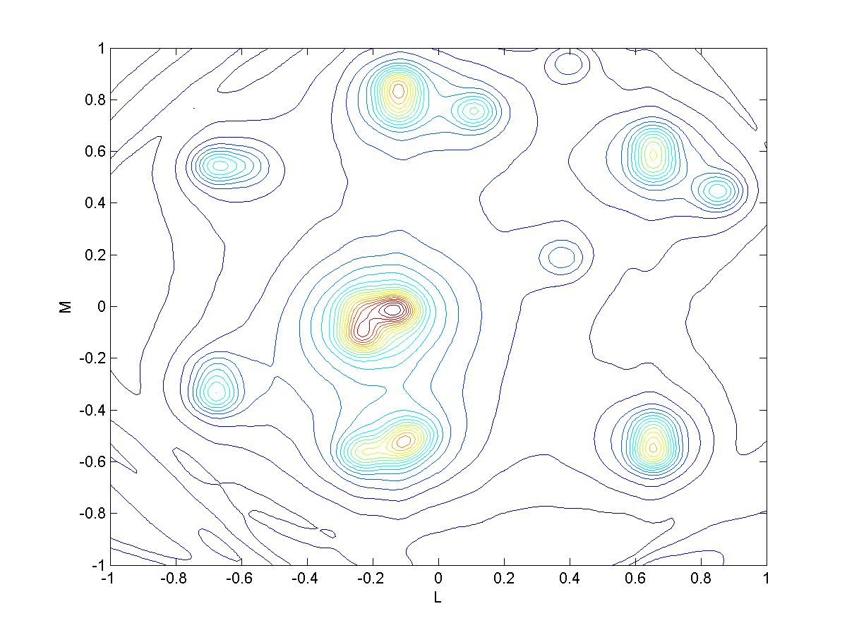
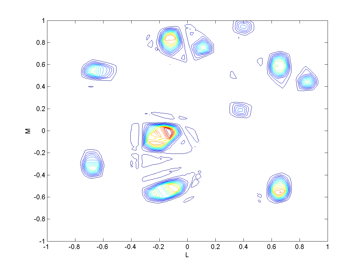
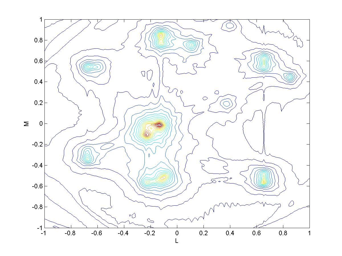
This section reports on ASSC algorithm performance compared to existing techniques (classic and MVDR) for the example discussed in (II). The ASSC parameters are and . Figure (4a) shows the original image that contains a few clusters of sources. Using the classic beamformer (Figure (4b)), the resulting image (classic dirty image) has wide peaks around each cluster of sources, and the noise is high. The ASSC classic beamformer yield a much quieter image (Figure (4c)). The MVDR (Figure (4d)) beamformer image has higher spatial resolution than the classic beamformer (as expected). The ASSC MVDR beamformer (Figure (4e)) has higher resolution than the MVDR and has the advantage of a quiet image.
III-B Strong out-of-FOV interference
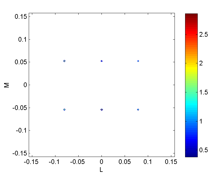
This section presents examples of a very strong interference times the power of the desired sources. Using an East-West array with antennas logarithmically spaced . Measurement was done every minute for a 12-hour period. The ASSC parameters used were (out of the available orientations ) and . Figure (5a) shows the original observed image with 6 point sources. The strong interference is not seen in the image (since the interferer is out of the field of view). The output of the classic and MVDR beamformer (dirty images) are shown in Figures (5b) and (5c) respectively. The entire image is smeared with the strong interferer sidelobes. The point sources are not seen. The output of the ASSC MVDR beamformer is shown in Figure (5d). The point sources are seen clearly and the strong interferer sidelobes do not appear in the image at all since only correlation matrices that are affected negligibly from the sidelobes are selected.
IV Summary
In this paper we introduced the ASSC beamformer, a method to combine rotating/many array measurements for interference suppression. The performance of the ASSC (classic and MVDR) were demonstrated and compared to the classic and MVDR beamformer. For interference dominant cases, the ASSC beamformer obtains images with higher spatial resolution and interference cancelation than either the classic or the MVDR beamformer.
References
- [1] G. Taylor, C. Carilli, and R. Perley, Synthesis Imaging in Radio-Astronomy. Astronomical Society of the Pacific, 1999.
- [2] A. Thompson, J. Moran, and G. Swenson, eds., Interferometry and Synthesis in Radio astronomy. John Wiley and Sons, 1986.
- [3] J. A. Högbom, “Aperture synthesis with nonregular distribution of intereferometer baselines,” Astron. Astrophys. Suppl, vol. 15, pp. 417–426, 1974.
- [4] T. Cornwell, “Multiscale CLEAN deconvolution of radio synthesis images,” IEEE Journal of Selected Topics in Signal Processing, vol. 2, pp. 793–801, Oct. 2008.
- [5] U. Rau, S. Bhatnagar, M. Voronkov, and T. Cornwell, “Advances in calibration and imaging techniques in radio interferometry,” Proceeding of the IEEE, vol. 97, pp. 1472–1481, Aug 2009.
- [6] A. Leshem and A. van der Veen, “Radio-astronomical imaging in the presence of strong radio interference,” IEEE Trans. on Information Theory, Special issue on information theoretic imaging, pp. 1730–1747, August 2000.
- [7] C. Ben-David and A. Leshem, “Parametric high resolution techniques for radio astronomical imaging,” IEEE Journal of Selected Topics in Signal Processing, vol. 2, pp. 670–684, Oct. 2008.
- [8] A. Leshem, A. van der Veen, and A. J. Boonstra, “Multichannel interference mitigation techniques in radio-astronomy,” The Astrophysical Journal Supplements, pp. 355–373, November 2000.
- [9] R. Levanda and A. Leshem, “Synthetic aperture radio telescopes,” IEEE Signal Processing Magazine, vol. 27, pp. 14–29, Jan. 2010.
- [10] A. van der Veen, A. Leshem, and A. Boonstra, “Array signal processing in radio-astronomy,” Experimental Astronomy, vol. 17, pp. 231–249, June 2004.
- [11] J. Capon, “High resolution frequency-wavenumber spectrum analysis,” Proceedings of the IEEE, pp. 1408–1418, 1969.
- [12] H. V. Trees, Optimum array processing. J. Wiley, 2002.