Multi-Agent Deployment for Visibility Coverage in Polygonal Environments with Holes

Abstract

This article presents a distributed algorithm for a group of robotic agents with omnidirectional vision to deploy into nonconvex polygonal environments with holes. Agents begin deployment from a common point, possess no prior knowledge of the environment, and operate only under line-of-sight sensing and communication. The objective of the deployment is for the agents to achieve full visibility coverage of the environment while maintaining line-of-sight connectivity with each other. This is achieved by incrementally partitioning the environment into distinct regions, each completely visible from some agent. Proofs are given of (i) convergence, (ii) upper bounds on the time and number of agents required, and (iii) bounds on the memory and communication complexity. Simulation results and description of robust extensions are also included.

I Introduction

Robots are increasingly being used for surveillance missions too dangerous for humans, or which require duty cycles beyond human capacity. In this article we design a distributed algorithm for deploying a group of mobile robotic agents with omnidirectional vision into nonconvex polygonal environments with holes, e.g., an urban or building floor plan. Agents are identical except for their unique identifiers (UIDs), begin deployment from a common point, possess no prior knowledge of the environment, and operate only under line-of-sight sensing and communication. The objective of the deployment is for the agents to achieve full visibility coverage of the environment while maintaining line-of-sight connectivity (at any time the agents’ visibility graph consists of a single connected component). We call this the Distributed Visibility-Based Deployment Problem with Connectivity. Once deployed, the agents may supply surveillance information to an operator through the ad-hoc line-of-sight communication network. A graphical description of our objective is given in Fig. 1.

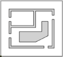
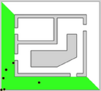
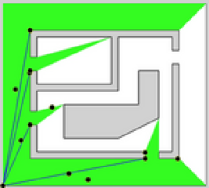
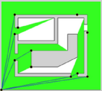
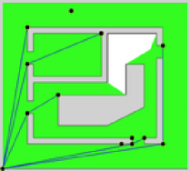
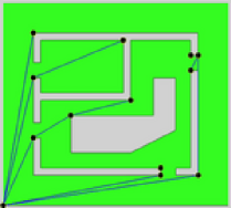
Figure 1: This sequence (left to right, top to bottom) shows a simulation run of the distributed visibility-based deployment algorithm described in Sec. VI. Agents (black disks) initially are colocated in the lower left corner of the environment. As the agents spread out, they claim areas of responsibility (green) which correspond to cells of the incremental partition tree ${\mathcal{T}}_{\mathcal{P}}$. Blue lines show line-of-sight connections between agents responsible for neighboring vertices of ${\mathcal{T}}_{\mathcal{P}}$. Once agents have settled to their final positions, every point in the environment is visibile to some agent and the agents form a line-of-sight connected network. An animation of this simulation can be viewed at http://motion.me.ucsb.edu/$\sim$karl/movies/dwh.mov .

Approaches to visibility coverage problems can be divided into two categories: those where the environment is known a priori and those where the environment must be discovered. When the environment is known a priori, a well-known approach is the Art Gallery Problem in which one seeks the smallest set of guards such that every point in a polygon is visible to some guard. This problem has been shown both NP-hard [1] and APX-hard [2] in the number of vertices $n$ representing the environment. The best known approximation algorithms offer solutions only within a factor of $O(\log g)$, where $g$ is the optimum number of agents [3]. The Art Gallery Problem with Connectivity is the same as the Art Gallery Problem, but with the additional constraint that the guards’ visibility graph must consist of a single connected component, i.e., the guards must form a connected network by line of sight. This problem is also NP-hard in $n$ [4]. Many other variations on the Art Gallery Problem are well surveyed in [5, 6, 7]. The classical Art Gallery Theorem, proven first in [8] by induction and in [9] by a beautiful coloring argument, states that $\lfloor\frac{n}{3}\rfloor$ vertex guards are always sufficient and sometimes necessary to cover a polygon with $n$ vertices and no holes. The Art Gallery Theorem with Holes, later proven independently by [10] and [11], states that $\lfloor\frac{n+h}{3}\rfloor$ point guards are always sufficient and sometimes necessary to cover a polygon with $n$ vertices and $h$ holes. If guard connectivity is required, [12] proved by induction and [13] by a coloring argument, that $\lfloor\frac{n-2}{2}\rfloor$ vertex guards are always sufficient and occasionally necessary for polygons without holes. We are not aware of any such bound for connected coverage of polygons with holes. For polygonal environments with holes, centralized camera-placement algorithms described in [14] and [15] take into account practical imaging limitations such as camera range and angle-of-incidence, but at the expense of being able to obtain worst-case bounds as in the Art Gallery Theorems. The constructive proofs of the Art Gallery Theorems rely on global knowledge of the environment and thus are not amenable to emulation by distributed algorithms.

One approach to visibiliy coverage when the environment must be discovered is to first use SLAM (Simultaneous Localization And Mapping) techniques [16] to explore and build a map of the entire environment, then use a centralized procedure to decide where to send agents. In [17], for example, deployment locations are chosen by a human user after an initial map has been built. Waiting for a complete map of the entire environment to be built before placing agents may not be desirable. In [18] agents fuse sensor data to build only a map of the portion of the environment covered so far, then heuristics are used to deploy agents onto the frontier of the this map, thus repeating this procedure incrementally expands the covered region. For any techniques relying heavily on SLAM, however, synchronization and data fusion can pose significant challenges under communication bandwidth limitations. In [19] agents discover and achieve visibility coverage of an environment not by building a geometric map, but instead by sharing only combinatorial information about the environment, however, the strategy focuses on the theoretical limits of what can be achieved with minimalistic sensing, thus the amount of robot motion required becomes impractical.

Most relevant to and the inspiration for the present work are the distributed visibility-based deployment algorithms, for polygonal environments without holes, developed recently by Ganguli et al [20, 21, 22]. These algorithms are simple, require only limited impact-based communication, and offer worst-case optimal bounds on the number of agents required. The basic strategy is to incrementally construct a so-called nagivation tree through the environment. To each vertex in the navigation tree corresponds a region of the the environment which is completely visible from that vertex. As agents move through the environment, they eventually settle on certain nodes of the navigation tree such that the entire environment is covered.

The contribution of this article is the first distributed deployment algorithm which solves, with provable performance, the Distributed Visibility-Based Deployment Problem with Connectivity in polygonal environments with holes. Our algorithm operates using line-of-sight communication and a so-called partition tree data structure similar to the navigation tree used by Ganguli et al as described above. The algorithms of Ganguli et al fail in polygonal environments with holes because branches of the navigation tree conflict when they wrap around one or more holes. Our algorithm, however, is able to handle such “branch conflicts”. Given at least $\lfloor\frac{n+2h-1}{2}\rfloor$ agents in an environment with $n$ vertices and $h$ holes, the deployment is guaranteed to achieve full visibility coverage of the environment in time $\mathcal{O}(n^{2}+nh)$, or time $\mathcal{O}(n+h)$ under certain technical conditions. We also prove bounds on the memory and communication complexity. The deployment behaves in simulations as predicted by the theory and can be extended to achieve robustness to agent arrival, agent failure, packet loss, removal of an environment edge (such as an opening door), or deployment from multiple roots.

This article is organized as follows. We begin with some technical definitions in Sec. II, then a precise statement of the problem and assumptions in Sec. III. Details on the agents’ sensing, dynamics, and communication are given in Sec. IV. Algorithm descriptions, including pseudocode and simulation results, are presented in Sec. V and Sec. VI. We conclude in Section VII.

II Notation and Preliminaries

We begin by introducing some basic notation. The real numbers are represented by ${\mathbb{R}}$. Given a set, say $A$, the interior of $A$ is denoted by $\operatorname{int}(A)$, the boundary by $\partial A$, and the cardinality by $|A|$. Two sets $A$ and $B$ are openly disjoint if $\operatorname{int}(A)\cap\operatorname{int}(B)=\emptyset$. Given two points $a,b\in{\mathbb{R}}^{2}$, $[a,b]$ is the closed segment between $a$ and $b$. Similarly, $]a,b[$ is the open segment between $a$ and $b$. The number of robotic agents is $N$ and each of these agents has a unique identifier (UID) taking a value in $\{0,\ldots,N-1\}$. Agent positions are $P=(p^{[0]},\ldots,p^{[N-1]})$, a tuple of points in ${\mathbb{R}}^{2}$. Just as $p^{[i]}$ represents the position of agent $i$, we use such superscripted square brackets with any variable associated with agent $i$, e.g., as in Table IV.

We turn our attention to the environment, visibility, and graph theoretic concepts. The environment $\mathcal{E}$ is polygonal with vertex set $V_{\mathcal{E}}$, edge set $E_{\mathcal{E}}$, total vertex count $n=|V_{\mathcal{E}}|=|E_{\mathcal{E}}|$, and hole count $h$. Given any polygon $c\subset\mathcal{E}$, the vertex set of $c$ is $V_{c}$ and the edge set is $E_{c}$. A segment $[a,b]$ is a diagonal of $\mathcal{E}$ if (i) $a$ and $b$ are vertices of $\mathcal{E}$, and (ii) $]a,b[\subset\operatorname{int}(\mathcal{E})$. Let $e$ be any point in $\mathcal{E}$. The point $e$ is visible from another point $e^{\prime}\in\mathcal{E}$ if $[e,e^{\prime}]\subset\mathcal{E}$. The visibility polygon $\mathcal{V}(e)\subset\mathcal{E}$ of $e$ is the set of points in $\mathcal{E}$ visible from $e$ (Fig. 2). The vertex-limited visibility polygon $\tilde{\mathcal{V}}(e)\subset\mathcal{V}$ is the visibility polygon $\mathcal{V}(e)$ modified by deleting every vertex which does not coincide with an environment vertex (Fig. 2). A gap edge of $\mathcal{V}(e)$ (resp. $\tilde{\mathcal{V}}(e)$) is defined as any line segment $[a,b]$ such that $]a,b[\subset\operatorname{int}(\mathcal{E})$, $[a,b]\subset\partial\mathcal{V}(e)$ (resp. $[a,b]\subset\partial\tilde{\mathcal{V}}(e)$), and it is maximal in the sense that $a,b\in\partial\mathcal{E}$. Note that a gap edge of $\tilde{\mathcal{V}}(e)$ is also a diagonal of $\mathcal{E}$. For short, we refer to the gap edges of $\mathcal{V}(e)$ as the visibility gaps of $e$.

Figure 2: In a simple nonconvex polygonal environment are shown examples of the visibility polygon (red, left) of a point observer (black disk), and the vertex-limited visibility polygon (red, right) of the same point.

A set $R\subset\mathcal{E}$ is star-convex if there exists a point $e\in R$ such that $R\subset\mathcal{V}(e)$. The kernel of a star-convex set $R$, is the set $\{e\in\mathcal{E}|R\subset\mathcal{V}(e)\}$, i.e., all points in $R$ from which all of $R$ is visible. The visibility graph $\mathcal{G}_{{\rm vis},\mathcal{E}}(P)$ of a set of points $P$ in environment $\mathcal{E}$ is the undirected graph with $P$ as the set of vertices and an edge between two vertices if and only if they are (mutually) visible. A tree is a connected graph with no simple cycles. A rooted tree is a tree with a special vertex designated as the root. The depth of a vertex in a rooted tree is the minimum number of edges which must be treversed to reach the root from that vertex. Given a tree $\mathcal{T}$, $V_{\mathcal{T}}$ is its set of vertices and $E_{\mathcal{T}}$ its set of edges.

III Problem Description and Assumptions

The Distributed Visibility-Based Deployment Problem with Connectivity which we solve in the present work is formally stated as follows:

Design a distributed algorithm for a network of autonomous robotic agents to deploy into an unmapped environment such that from their final positions every point in the environment is visible from some agent. The agents begin deployment from a common point, their visibility graph $\mathcal{G}_{{\rm vis},\mathcal{E}}(P)$ is to remain connected, and they are to operate using only information from local sensing and line-of-sight communication.

By local sensing we intend that each agent is able to sense its visibility gaps and relative positions of objects within line of sight. Additionally, we make the following main assumptions:

1. The environment $\mathcal{E}$ is static and consists of a simple polygonal outer boundary together with disjoint simple polygonal holes. By simple we mean that each polygon has a single boundary component, its boundary does not intersect itself, and the number of edges is finite.

2. Agents are identical except for their UIDs ($0,\ldots,N-1$).

3. Agents do not obstruct visibility or movement of other agents.

4. Agents are able to locally establish a common reference frame.

5. There are no communication errors nor packet losses.

Later, in Sec. VI-F we will describe how our nominal deployment algorithm can be extended to relax some assumptions.

IV Network of Visually-Guided Agents

In this section we lay down the sensing, dynamic, and communication model for the agents. Each agent has “omnidirectional vision” meaning an agent possesses some device or combination of devices which allows it to sense within line of sight (i) the relative position of another agent, (ii) the relative position of a point on the boundary of the environment, and (iii) the gap edges of its visibility polygon.

For simplicity, we model the agents as point masses with first order dynamics, i.e., agent $i$ may move through $\mathcal{E}$ according to the continuous time control system

$$\dot{p}^{[i]}=u^{[i]},$$ (1)

where the control $u^{[i]}$ is bounded in magnitude by $u_{\rm max}$. The control action depends on time, values of variables stored in local memory, and the information obtained from communication and sensing. Although we present our algorithms using these first order dynamics, the crucial property for convergence is only that an agent is able to navigate along any (unobstructed) straight line segment between two points in the environment $\mathcal{E}$, thus the deployment algorithm we describe is valid also for higher order dynamics.

The agents’ communication graph is precisely their visibility graph $\mathcal{G}_{{\rm vis},\mathcal{E}}(P)$, i.e., any visibility neighbors (mutually visible agents) may communicate with each other. Agents may send their messages using, e.g., UDP (User Datagram Protocol). Each agent ($i=0,\ldots,N-1$) stores received messages in a FIFO (First-In-First-Out) buffer In_Buffer^[i] until they can be processed. Messages are sent only upon the occurrence of certain asynchronous events and the agents’ processors need not be synchronized, thus the agents form an event-driven asynchronous robotic network similar to that described, e.g., in [23]. In order for two visibility neighbors to establish a common reference frame, we assume agents are able to solve the correspondence problem: the ability to associate the messages they receive with the corresponding robots they can see. This may be accomplished, e.g., by the robots performing localization, however, as mentioned in Sec. I, this might use up limited communication bandwidth and processing power. Simpler solutions include having agents display different colors, “license plates”, or periodic patterns from LEDs [24].

V Incremental Partition Algorithm

We introduce a centralized algorithm to incrementally partition the environment $\mathcal{E}$ into a finite set of openly disjoint star-convex polygonal cells. Roughly, the algorithm operates by choosing at each step a new vantage point on the frontier of the uncovered region of the environment, then computing a cell to be covered by that vantage point (each vantage point is in the kernel of its corresponding cell). The frontier is pushed as more and more vantage point - cell pairs are added until eventually the entire environment is covered. The vantage point - cell pairs form a directed rooted tree structure called the partition tree ${\mathcal{T}}_{\mathcal{P}}$. This algorithm is a variation and extension of an incremental partition algorithm used in [22], the main differences being that we have added a protocol for handling holes and adapted the notation to better fit the added complexity of handling holes. The deployment algorithm to be described in Sec. VI is a distributed emulation of the centralized incremental partition algorithm we present here.

Before examining the precise pseudocode Table I, we informally step through the incremental partition algorithm for the simple example of Fig. 3a-f. This sequence shows the environment partition together with corresponding abstract representations of the partition tree ${\mathcal{T}}_{\mathcal{P}}$. Each vertex of ${\mathcal{T}}_{\mathcal{P}}$ is a vantage point - cell pair and edges are based on cell adjacency. Given any vertex of ${\mathcal{T}}_{\mathcal{P}}$, say $(p_{\xi},c_{\xi})$, $\xi$ is the PTVUID (Partition Tree Vertex Unique IDentifier). The PTVUID of a vertex at depth $d$ is a $d$-tuple, e.g., (1), (2,1), or (1,1,1). The symbol $\emptyset$ is used as the root’s PTVUID. The algorithm begins with the root vantage point $p_{\emptyset}$. The cell of $p_{\emptyset}$ is the grey shaded region $c_{\emptyset}$ in Fig. 3a, which is the vertex-limited visibility polygon $\tilde{\mathcal{V}}(p_{\emptyset})$. According to certain technical criteria, made precise later, child vantage points are chosen on the endpoints of the unexplored gap edges. In Fig. 3a, dashed lines show the unexplored gap edges of $c_{\emptyset}$. Selecting $p_{(1)}$ as the next vantage point, the corresponding cell $c_{(1)}$ becomes the portion of $\tilde{\mathcal{V}}(p_{(1)})$ which is across the parent gap edge and extends away from the parent’s cell. The vantage point $p_{(2)}$ and its cell $c_{(2)}$ are generated in the same way. There are now three vertices, $(p_{\emptyset},c_{\emptyset})$, $(p_{(1)},c_{(1)})$, and $(p_{(2)},c_{(2)})$ in ${\mathcal{T}}_{\mathcal{P}}$ (Fig. 3b). In a similar manner, two more vertices, $(p_{(2,1)},c_{(2,1)})$ and $(p_{(2,1,1)},c_{(2,1,1)})$, have been added in Fig. 3c. An intersection of positive area is found between cell $c_{(2,1,1)}$ and the cell of another branch of ${\mathcal{T}}_{\mathcal{P}}$, namely $c_{(1)}$. To solve this branch conflict, the cell $c_{(2,1,1)}$ is discarded and a special marker called a phantom wall (thick dashed line in Fig. 3d) is placed where its parent gap edge was. A phantom wall serves to indicate that no branch of ${\mathcal{T}}_{\mathcal{P}}$ should cross a particular gap edge. The vertex $(p_{(1,2)},c_{(1,2)})$ added in Fig. 3e thus can have no children. Finally, Fig. 3f shows the remaining vertices $(p_{(1,1)},c_{(1,1)})$ and $(p_{(1,1,1)},c_{(1,1,1)})$ added to ${\mathcal{T}}_{\mathcal{P}}$ so that the entire environment is covered and the algorithm terminates.

Figure 3: This simple example shows how the incremental partition algorithm of Table I progresses (a)-(f). Cell vantage points are shown by black disks. The portion of the environment $\mathcal{E}$ covered at each stage is shown in grey (left) along with a corresponding abstract depiction of the partition tree (right). A phantom wall (thick dashed line), shown first in (d), comes about when there is a branch conflict, i.e., when cells from different branches of the partition tree ${\mathcal{T}}_{\mathcal{P}}$ are not openly disjoint. The final partition can be used to triangulate the environment as shown in Fig. 4.

Figure 3: (continuation)

TABLE I: Centralized Incremental Partition Algorithm

  INCREMENTAL_PARTITION$(\mathcal{E},p_{\emptyset})$

1:  {Compute and Insert Root Vertex into ${\mathcal{T}}_{\mathcal{P}}$}

2:  $c_{\emptyset}\leftarrow\tilde{\mathcal{V}}(p_{\emptyset})$;

3:  for each gap edge $g$ of $c_{\emptyset}$ do

4:     label $g$ as unexplored in $c_{\emptyset}$;

5:  insert $(p_{\emptyset},c_{\emptyset})$ into ${\mathcal{T}}_{\mathcal{P}}$;

6:  {Main Loop}

7:  while  any cell in ${\mathcal{T}}_{\mathcal{P}}$ has unexplored gap edges  do

8:     $c_{\zeta}\leftarrow$ any cell in ${\mathcal{T}}_{\mathcal{P}}$ with unexplored gap edges;

9:     $g\leftarrow$ any unexplored gap edge of $c_{\zeta}$;

10:     $(p_{\xi},c_{\xi})\leftarrow$ CHILD$(\mathcal{E},{\mathcal{T}}_{\mathcal{P}},\zeta,g)$; {See Tab. II}

11:     {Check for Branch Conflicts}

12:     if  there exists any cell $c_{\xi^{\prime}}$ in ${\mathcal{T}}_{\mathcal{P}}$ which is in branch conflict with $c_{\xi}$  then

13:        discard $(p_{\xi},c_{\xi})$;

14:        label $g$ as phantom_wall in $c_{\zeta}$;

15:     else

16:        insert $(p_{\xi},c_{\xi})$ into ${\mathcal{T}}_{\mathcal{P}}$;

17:        label $g$ as child in $c_{\zeta}$;

18:  return ${\mathcal{T}}_{\mathcal{P}}$;

 

TABLE II: Incremental Partition Subroutine

  CHILD$(\mathcal{E},{\mathcal{T}}_{\mathcal{P}},\zeta,g)$

1:  $\xi\leftarrow\operatorname{successor}(\zeta,i)$, where $g$ is the $i$th nonparent gap edge of $c_{\zeta}$ counterclockwise from $p_{\zeta}$;

2:  if  $|V_{c_{\xi}}|>3$ then

3:     enumerate $c_{\zeta}$’s vertices $1,2,3,\ldots$ counterclockwise from $p_{\zeta}$;

4:  else

5:     enumerate $c_{\zeta}$’s vertices so that $p_{\zeta}$ is assigned $1$ and the remaining vertices of $c_{\zeta}$ are assigned $2$ and $3$ such that the vertex assigned $3$ is on the parent gap edge of $c_{\zeta}$;

6:  $p_{\rm\xi}\leftarrow$ vertex on $g$ assigned an odd integer in the enumeration;

7:  $c_{\xi}\leftarrow\tilde{\mathcal{V}}(p_{\xi})$;

8:  truncate $c_{\xi}$ at $g$ such that only the portion remains which is across $g$ from $p_{\zeta}$;

9:  delete from $c_{\xi}$ any vertices which lie across a phantom wall from $p_{\xi}$;

10:  for  each gap edge $g^{\prime}$ of $c_{\xi}$  do

11:     if  $g^{\prime}==g$  then

12:        label $g^{\prime}$ as parent in $c_{\xi}$;

13:     else if  $g^{\prime}$ coincides with an existing phantom wall  then

14:        label $g^{\prime}$ as phantom_wall in $c_{\xi}$;

15:     else

16:        label $g^{\prime}$ as unexplored in $c_{\xi}$;

17:  return $(p_{\xi},c_{\xi})$;

 

Figure 4: The partition tree produced by the centralized incremental partition algorithm of Table I or the distributed deployment algorithm of Table VI can be used to triangulate an environment, as shown here for the simple example of Fig. 3. The triangulation is constructed by drawing diagonals (dashed lines) from each vantage point (black disks) to the visible environment vertices in its cell.

Now we turn our attention to the pseudocode Table I for a precise description of the algorithm. The input is the environment $\mathcal{E}$ and a single point $p_{\emptyset}\in V_{\mathcal{E}}$. The output is the partition tree ${\mathcal{T}}_{\mathcal{P}}$. We have seen that each vertex of the partition tree is a vantage point - cell pair. In particular, a cell is a data structure which stores not only a polygonal boundary, but also a label on each of the polygon’s gap edges. A gap edge label takes one of four possible values: parent, child, unexplored, or phantom wall. These labels allow the following exact definition of the partition tree.

Definition V.1 (Partition Tree ${\mathcal{T}}_{\mathcal{P}}$)

The directed rooted partition tree ${\mathcal{T}}_{\mathcal{P}}$ has

1. vertex set consisting of vantage point - cell pairs produced by the incremental partition algorithm of Table I, and

2. a directed edge from vertex $(p_{\zeta},c_{\zeta})$ to vertex $(p_{\xi},c_{\xi})$ if and only if $c_{\zeta}$ has a child gap edge which coincides with a parent gap edge of $c_{\xi}$.

Stepping through the pseudocode Table I, lines 1-5 compute and insert the root vertex $(p_{\emptyset},c_{\emptyset})$ into ${\mathcal{T}}_{\mathcal{P}}$. Upon entering the main loop at line 7, line 8 selects a cell $c_{\zeta}$ arbitrarily from the set of cells in ${\mathcal{T}}_{\mathcal{P}}$ which have unexplored gap edges. Line 9 selects an arbitrary unexplored gap edge $g$ of $c_{\zeta}$. The next vantage point candidate will be placed on an endpoint of $g$ by a call on line 10 to the CHILD function of Table II. The PTVUID $\xi$ is computed by the successor function on line 1 of Table II. For any $d$-tuple $\zeta$ and positive integer $i$, $\operatorname{successor}(\zeta,i)$ is simply the $(d+1)$-tuple which is the concatenation of $\zeta$ and $i$, e.g., $\operatorname{successor}((2,1),1))=(2,1,1)$. The CHILD function constructs a candidate vantage point $p_{\xi}$ and cell $c_{\xi}$ as follows. In the typical case, when the parent cell $c_{\zeta}$ has more than three edges, $c_{\zeta}$’s vertices are enumerated counterclockwise from $p_{\zeta}$, e.g., as $c_{\emptyset}$’s vertices in Fig. 3a or Fig. 6. In the special case of $c_{\zeta}$ being a triangle, e.g., as the triangular cells in Fig. 6, $c_{\zeta}$’s vertices are enumerated such that the $3$ lands on $c_{\zeta}$’s parent gap edge. The vertex of $g$ which is odd in the enumeration is selected as $p_{\xi}$. Occasionally there may be double vantage points (colocated), e.g., as $p_{(2)}$ and $p_{(3)}$ in Fig. 6. We will see in Sec. V-A that this parity-based vantage point selection scheme is important for obtaining a special subset of the vantage points called the sparse vantage point set. Returning to Table I, the final portion of the main loop, lines 11-17, checks whether $c_{\xi}$ is in branch conflict or $(p_{\xi},c_{\xi})$ should be added permanently to ${\mathcal{T}}_{\mathcal{P}}$. A cell $c_{\xi}$ is in branch conflict with another cell $c_{\xi^{\prime}}$ if and only if $c_{\xi}$ and $c_{\xi^{\prime}}$ are not openly disjoint (see Fig. 5). The main algorithm terminates when there are no more unexplored gap edges in ${\mathcal{T}}_{\mathcal{P}}$.

Figure 5: The incremental partition algorithm of Table I and distributed deployment algorithm of Table VI may discard a cell $c_{\xi}$ if it is in branch conflict with another cell $c_{\xi^{\prime}}$ already in the partition tree, i.e., when $c_{\xi}$ and $c_{\xi^{\prime}}$ and are not openly disjoint. In these three examples, blue represents one cell $c_{\xi}$, red another cell $c_{\xi^{\prime}}$, and purple their intersection $c_{\xi}\cap c_{\xi^{\prime}}$. A cell can even conflict with it’s own parent if they enclose a hole as in (c).

An important difference between our incremental partition algorithm and that of Ganguli et al [22] is that the set of cells computed by our incremental partition is not unique. This is because the freedom in choosing cell $c_{\zeta}$ and gap $g$ on lines 8-9 of Table I allows different executions of the algorithm to fill the same part of the environment with different branches of ${\mathcal{T}}_{\mathcal{P}}$. This may result in different sets of phantom walls as well. A phantom wall is only created on line 14 of Table I when there is a branch conflict. This discarding may seem computationally wasteful because the environment could just be made simply connected by choosing $h$ phantom walls (one for each hole) prior to executing the algorithm. Such an approach, however, would not be amenable to distributed emulation without a priori knowledge of the environment.

Figure 6: The example used in Fig. 3 showed a typical incremental partition in which there were neither double vantage points nor any triangular cells. This example, on the other hand, shows these special cases. Disks, black or white, show vantage points produced by the incremental partition algorithm of Table I. Integers show enumerations of the cells used for the parity-based vantage point selection scheme. The double vantage points $p_{(2)}$ and $p_{(3)}$ are colocated. The cells $c_{(2)}$, $c_{(3)}$, $c_{(2,1)}$, $c_{(3.1)}$, $c_{(2,1,1)}$, and $c_{(3,1,1)}$ are triangular. The vantage points colored black are the sparse vantage points found by the postprocessing algorithm of Table III. Under the distributed deployment algorithm of Table VI, robotic agents position themselves at sparse vantage points.

The following important properties we prove for the incremental partition algorithm are similar to properties we obtain for the distributed deployment algorithm in Sec. VI.

Lemma V.2 (Star-Convexity of Partition Cells)

Any partition tree vertex $(p_{\xi},c_{\xi})$ constructed by the incremental partition algorithm of Table I, has the properties that

1. the cell $c_{\xi}$ is star-convex, and

2. the vantage point $p_{\xi}$ is in the kernel of $c_{\xi}$.

Proof:

Given a star-convex set, say $S$, let $K$ be the kernel of $S$. Suppose that we obtain a new set $S^{\prime}$ by truncating $S$ at a single line segment $l$ who’s endpoints lie on the boundary $\partial S$. It is easy so see that the kernel of $S^{\prime}$ contains $K\cap S^{\prime}$, thus $S^{\prime}$ must be star-convex if $K\cap S^{\prime}$ is nonempty. Indeed $l$ could not possibly block line of sight from any point in $K\cap S^{\prime}$ to any point $p$ in $S^{\prime}$, otherwise $p$ would have been truncated. Inductively, we can obtain a set $S^{\prime}$ by truncating the set $S$ at any finite number of line segments and the kernel of $S^{\prime}$ will be a superset of $S^{\prime}\cap K$. Now consider a partition tree vertex $(p_{\xi},c_{\xi})$. By definition, the visibility polygon $\mathcal{V}(p_{\xi})$ is star-convex and $p_{\xi}$ is in the kernel. By the above reasoning, the vertex-limited visibility polygon $\tilde{\mathcal{V}}(p_{\xi})$ is also star-convex and has $p_{\xi}$ in its kernel because $\tilde{\mathcal{V}}(p_{\xi})$ can be obtained from $\mathcal{V}(p_{\xi})$ by a finite number of line segment truncations (lines 8 and 9 of Table II). Likewise, $c_{\xi}$ must be star-convex with $p_{\xi}$ in its kernel because $c_{\xi}$ is obtained from $\tilde{\mathcal{V}}(p_{\xi})$ by a finite number of line segment truncations at the parent gap edge and phantom walls. ∎

Theorem V.3 (Properties of the Incremental Partition Algorithm)

Suppose the incremental partition algorithm of Table I is executed on an environment $\mathcal{E}$ with $n$ vertices and $h$ holes. Then

1. the algorithm returns in finite time a partition tree ${\mathcal{T}}_{\mathcal{P}}$ such that every point in the environment is visible to some vantage point,

2. the visibility graph of the vantage points $\mathcal{G}_{{\rm vis},\mathcal{E}}(\{p_{\xi}|(p_{\xi},c_{\xi})\in{\mathcal{T}}_{\mathcal{P}}\})$ consists of a single connected component,

3. the final number of vertices in ${\mathcal{T}}_{\mathcal{P}}$ (and thus the total number of vantage points) is no greater than $n+2h-2$,

4. there exist environments where the final number of vertices in ${\mathcal{T}}_{\mathcal{P}}$ is equal to the upper bound $n+2h-2$, and

5. the final number of phantom walls is precisely $h$.

Proof:

We prove the statements in order. The algorithm processes unexplored gap edges one by one and terminates when there are no more unexplored gap edges. Once an unexplored gap edge has been processed, it is never processed again because its label changes to phantom_ wall or child. Gap edges of cells are diagonals of the environment and there are no more than $\binom{n}{2}=\frac{n^{2}-n}{2}$ possible diagonals, which is finite, therefore the algorithm must terminate in finite time. Lemma V.2 guarantees that if the entire environment is covered by cells of ${\mathcal{T}}_{\mathcal{P}}$, then every point is visible to some vantage point. Suppose the final set of cells does not cover the entire environment. Then there must be a portion of the environment which is topologically isolated from the rest of the environment by phantom walls, otherwise an unexplored gap edge would have expanded into that region. However, this would mean that a phantom wall was created at the parent gap edge of a candidate cell which was not in branch conflict. This is not possible because a phantom wall is only ever created if there is a branch conflict (lines 12-14 Table I). This completes the proof of statement (i).

Statement (ii) follows from Lemma V.2 together with the fact that every vantage point is placed on the boundary of its parent’s cell. Given two vantage points in ${\mathcal{T}}_{\mathcal{P}}$, say $p_{\xi}$ and $p_{\xi^{\prime}}$, a path through $\mathcal{G}_{{\rm vis},\mathcal{E}}(\{p_{\xi}|(p_{\xi},c_{\xi})\in{\mathcal{T}}_{\mathcal{P}}\})$ from $p_{\xi}$ to $p_{\xi^{\prime}}$ can be constructed as follows. Follow parent-child visibility links up to the root vantage point $p_{\emptyset}$, then follow parent-child visibility links from $p_{\emptyset}$ down to $p_{\xi^{\prime}}$. Since such a path can always be constructed between any pair of vantage points, $\mathcal{G}_{{\rm vis},\mathcal{E}}(\{p_{\xi}|(p_{\xi},c_{\xi})\in{\mathcal{T}}_{\mathcal{P}}\})$ must consist of a single connected component.

For statement (iii), we triangulate $\mathcal{E}$ by triangulating the cells of ${\mathcal{T}}_{\mathcal{P}}$ individually as in Fig. 4. Each cell $c_{\xi}$ is triangulated by drawing diagonals from $p_{\xi}$ to the vertices of $c_{\xi}$. The total number of triangles in any triangulation of a polygonal environment with holes is $n+2h-2$ (Lemma 5.2 in [6]). Since there is at least one triangle per cell and at most one vantage point per cell, the number of vantage points cannot exceed the maximum number of triangles $n+2h-2$.

Statement (iv) is proven by the example in Fig. 7a.

For statement (v), we argue topologically. Suppose the final number of phantom walls were less than $h$. Then somewhere two branches of the parition tree must share a gap edge with no phantom wall separating them. If this shared gap edge is not a phantom wall, it must be either (1) a child in branch conflict, or (2) unexplored. Either way, the algorithm would have tried to create a cell there but then deleted it and created a phantom wall; a contradiction. Now suppose there were more than $h$ phantom walls. Then a cell would be topologically isolated by phantom walls from the rest of the environment. This is not possible because phantom walls can never be created at the parent-child gap edge between two cells. Since the final number of phantom walls can be neither less nor greater than $h$, it must be $h$.

∎

Figure 7: (a) An example of when the final number of vantage points in ${\mathcal{T}}_{\mathcal{P}}$ is equal to the upper bound $n+2h-2$ given in Theorem V.3. (b) An example of when the number of points in ${\mathbb{R}}^{2}$ where at least one sparse vantage point is located is equal to the upper bound $\left\lfloor\frac{n+2h-1}{2}\right\rfloor$ given in Theorems V.5 and VI.4.

V-A A Sparse Vantage Point Set

Suppose we were to deploy robotic agents onto the vantage points produced by the incremental partition algorithm (one agent per vantage point). Then, as Theorem V.3 guarantees, we would achieve our goal of complete visibility coverage with connectivity. The number of agents required would be no greater than the number of vantage points, namely $n+2h-2$. This upper bound, however, can be greatly improved upon. In order to reduce the number of vantage points agents must deploy to, the postprocessing algorithm in Table III takes the partition tree output by the incremental partition algorithm and labels a subset of the vantage points called the sparse vantage point set. Starting at the leaves of the partition tree and working towards the root, vantage points are labeled either nonsparse or sparse according to criterion on line 2 of Table III. As proven in Theorem V.5 below, the sparse vantage points are suitable for the coverage task and their cardinality has a much better upper bound than the full set of vantage points. All the vantage points in the example of Fig. 3 are sparse. Fig. 6 shows an example of when only a proper subset of the vantage points is sparse.

TABLE III: Postprocessing of Partition Tree

  LABEL_VANTAGE_POINTS$(\mathcal{E},{\mathcal{T}}_{\mathcal{P}})$

1:  while  there exists a vantage point $p_{\xi}$ in ${\mathcal{T}}_{\mathcal{P}}$ such that $p_{\xi}$ has not yet been labeled          and $\bigl{(}$ $p_{\xi}$ is at a leaf or all child vantage points of $p_{\xi}$ have been labeled $\bigr{)}$  do

2:     if  $|V_{c_{\xi}}|==3$ and $p_{\xi}$ has exactly one child vantage point labeled sparse  then

3:        label $p_{\xi}$ as nonsparse;

4:     else

5:        label $p_{\xi}$ as sparse;

 

Lemma V.4 (Properties of a Child Vantage Point of a Triangular Cell)

Let $(p_{\xi},c_{\xi})$ be a partition tree vertex constructed by the incremental partition algorithm of Table I and suppose $c_{\xi}$ has a parent cell $c_{\zeta}$ which is a triangle. Then $p_{\xi}$ is in the kernel of $p_{\zeta}$. Furthermore, if $p_{\zeta}$ has a parent vantage point $p_{\zeta^{\prime}}$ (the grandparent of $p_{\xi}$), then $p_{\xi}$ is visible to $p_{\zeta^{\prime}}$.

Proof:

The kernel of a triangular (and thus convex) cell $c_{\zeta}$ is all of $c_{\zeta}$. By Lemma V.2, $p_{\zeta^{\prime}}$ is in the kernel of $c_{\zeta^{\prime}}$. According to the parity-based vantage point selection scheme (line 5 of Table II), $p_{\xi}$ is located at a point common to $c_{\zeta^{\prime}}$, $c_{\zeta}$, and $c_{\xi}$, therefore $p_{\xi}$ is in the kernel of $c_{\zeta}$ and visible to $c_{\zeta^{\prime}}$. ∎

Theorem V.5 (Properties of the Sparse Vantage Point Set)

Suppose the incremental partition algorithm of Table I is executed to completion on an environment $\mathcal{E}$ with $n$ vertices and $h$ holes and the vantage points of the resulting partition tree are labeled by the algorithm in Table III. Then

1. every point in the environment is visible to some sparse vantage point,

2. the visibility graph of the sparse vantage points $\mathcal{G}_{{\rm vis},\mathcal{E}}(\{p_{\xi}|(p_{\xi},c_{\xi})\in{\mathcal{T}}_{\mathcal{P}}\})$ consists of a single connected component,

3. the number of points in ${\mathbb{R}}^{2}$ where at least one sparse vantage point is located is no greater than $\left\lfloor\frac{n+2h-1}{2}\right\rfloor$, and

4. there exist environments where the upper bound $\left\lfloor\frac{n+2h-1}{2}\right\rfloor$ in (iii) is met.

Proof:

Statements (i) and (ii) follow directly from Lemma V.4 together with statements (i) and (ii) of Theorem V.3.

For statement (iii) we use a triangulation argument similar to that used in [22] for environments without holes. We use the same triangulation as in the proof of Theorem V.3 (Fig. 4). The total number of triangles in any triangulation of a polygonal environment with holes is $n+2h-2$ (Lemma 5.2 in [6]). Suppose we can assign at least one unique triangle to $p_{\emptyset}$ whenever $p_{\emptyset}$ is sparse and at least two unique triangles to all other sparse vantage point locations. Let $N_{\rm sparse}$ be the number of sparse vantage point locations. Setting $2(N_{\rm sparse}-1)+1=2N_{\rm sparse}-1$ to be less or equal to the total number of triangles $n+2h-2$ and solving for $N_{\rm sparse}$ gives the desired bound

$$N_{\rm sparse}\leq\left\lfloor\frac{(n+2h-2)+1}{2}\right\rfloor=\left\lfloor\frac{n+2h-1}{2}\right\rfloor.$$

Indeed we can make such an assignment of triangles to sparse vantage point locations. Our argument relies on the parity-based vantage point selection scheme and the criterion for labeling a vantage point as sparse on line 2 of Table III. To any sparse vantage point location, say of $p_{\xi}$ other than the root, we assign one triangle in the parent cell. The triangle in the parent cell is the triangle formed by its parent gap edge together with its parent’s vantage point. To each sparse vantage point location, say of $p_{\xi}$, including the root, we assign additionally one triangle in the cell $c_{\xi}$. If $c_{\xi}$ has no children, then any triangle in $c_{\xi}$ can be assigned to $p_{\xi}$. If $c_{\xi}$ has children (in which case it must have greater than one triangle) we need to check that it has more triangles than child vantage point locations with odd parity. Suppose $c_{\xi}$ has an even number of edges. Then this number of edges can be written $2m$ where $m\geq 2$. The number of triangles in $c_{\xi}$ is $2m-2$ and the number of odd parity vertices in $c_{\xi}$ where child vantage points could be placed is $m-1$. This means at most $m-1$ triangles in $c_{\xi}$ are assigned to odd parity child vantage point locations, which leaves $(2m-2)-(m-1)=m-1\geq 1$ triangles to be assigned to the location of $p_{\xi}$. The case of $c_{\xi}$ having an odd number of edges is proven analogously.

Statement (iv) is proven by the example in Fig. 7.

∎

VI Distributed Deployment Algorithm

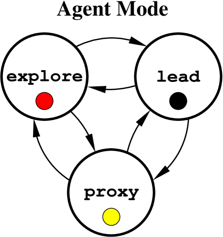
Figure 8: (a) In the distributed deployment algorithm of Table VI, each agent may switch between lead, proxy, and explore mode based on certain asynchronous events. Leader agents are responsible for maintaining a distributed representation of the partition tree ${\mathcal{T}}_{\mathcal{P}}$, proxies help establish communication for solving branch conflicts, and explorers systematically navigate through ${\mathcal{T}}_{\mathcal{P}}$ in search of opportunities to become a leader or proxy. The agent mode color code is used also in Fig. 10 and 12. (b) Even if a pair of leader agents (black) are not mutually visible, their cells ($c_{\xi}$ and $c_{\xi^{\prime}}$) may intersect as in Fig. 5, shown here abstractly by a Venn diagram. Sending a proxy agent (yellow), on a proxy tour around one of the cell boundaries guarantees it will enter the cells’ intersection so that communication between leaders can be proxied. The leaders can then establish a local common reference frame and compare cell boundaries in order to solve branch conflicts.

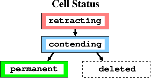
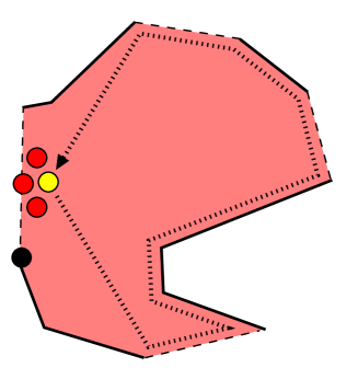
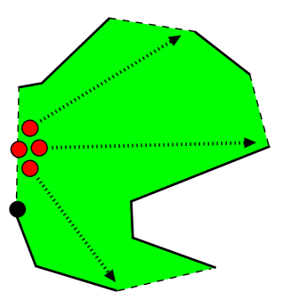
Figure 9: (a) In the distributed deployment algorithm of Table VI, any cell in a leader’s memory has a status which takes the value retracting, contending, or permanent. (b) Each cell status is initially retracting. The status of a retracting cell is advanced to contending after the execution of a proxy tour in which the cell is truncated as necessary to ensure no branch conflict with any permanent cells. (c) In a second proxy tour, a contending cell is deleted if it is found to be in branch conflict with another contending cell of smaller PTVUID (according to total ordering Def. VI.2), otherwise its status is advanced to permanent. (d) Only when a cell has attained status permanent can any child cells be added at its unexplored gap edges (continued in Fig. 10). The cell status color code is used in Fig. 10 as well as 12.

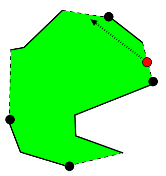
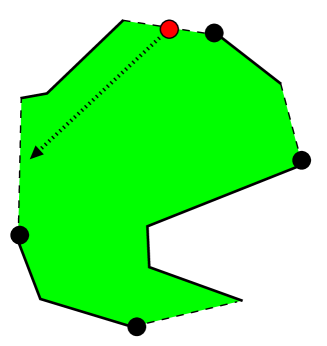
Figure 10: Color codes correspond to those in Fig. 8 and 9. (a,b) Once a cell has status permanent, arriving explorer agents can be sent to become leaders at child gap edges. (c-f) Any remaining explorer agents continue systematically navigating the partition tree in search of leader or proxy tasks they could perform .

Figure 11: In the distributed deployment algorithm of Table VI, explorer agents search the partition tree ${\mathcal{T}}_{\mathcal{P}}$ depth-first for leader or proxy tasks they could perform. An agent in a cell, say $c_{\xi}$, can always order the gap edges of $c_{\xi}$, e.g., counterclockwise from the parent gap edge. The depth-first search progresses by the explorer agent always moving to the next unvisited child or unexplored gap edge in that ordering. The agent thus moves from cell to cell deeper and deeper until a leaf (a vertex with no children) is found. Once at a leaf, the agent backtracks to the most recent vertex with unvisited child or unexplored gap edges and the process continues. As an example, (left) integers (not to be confused with PTVUIDs) shows the depth-first order an agent would visit the vertices of ${\mathcal{T}}_{\mathcal{P}}$ in Fig. 3f if the gap edges in each cell were ordered couterclockwise from the parent gap edge. If the agent instead uses a gap edge ordering cyclically shifted by one, then (right) shows the different resulting depth-first order. If each agent uses a different gap edge ordering, e.g., cyclically shifted by their UID, then different branches of ${\mathcal{T}}_{\mathcal{P}}$ are explored in parallel and the deployment tends to cover the environment more quickly. Cf. Fig. 10.

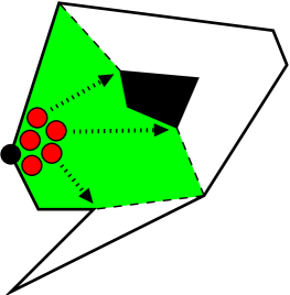
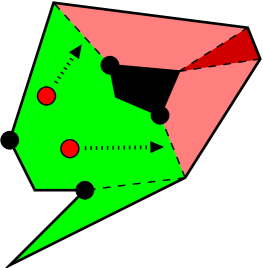
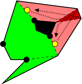
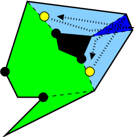
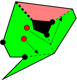
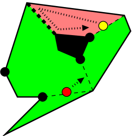
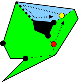
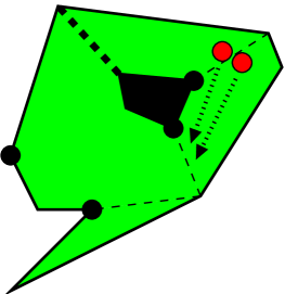
Figure 12: With color codes from Fig. 8 and 9, here is a simple example of agents executing the distributed deployment algorithm of Table VI. (a) Agents enter the environment and the leader initializes the root cell to status permanent because no branch conflicts could possibly exist yet. Explorer agents move out to become leaders of child cells. (b) The lower child cell is initialized with status permanent because it has no gap edges and thus cannot be in branch conflict. The upper two child cells are initialized to retracting because they could be in branch conflict at unexplored gap edges; indeed there is a branch conflict at the dark red overlap region. The remaining explorer agents continue moving out to the new cells. (c) Once the explorers reach the retracting cells, they become proxies and run tours around the cells to check for branch conflict with permanent cells. (d) After the first proxy tours, the child cells’ statuses are advanced to contending and each proxy run a second tour. (e) During the second proxy tours, the branch conflict is detected between contending cells and the cell with higher PTVUID is deleted. The agents that were in the deleted cell move back up the partition tree and continue exploring depth-first. The other proxy becomes a leader of a new child cell initialized to retracting. (f) One of the explorers arrives at the retracting cell and begins a proxy tour to advance the cell to contending. (g) The proxy runs a second tour and advances the cell to permanent and the partition is completed. (h) Remaining explorers continue navigating the partition tree depth-first in search of tasks; this adds robustness because they will be able to fill in anywhere an agent may fail or a door may open.

In this section we describe how a group of mobile robotic agents can distributedly emulate the incremental partition and vantage point labeling algorithms of Sec. V, thus solving the Distributed Visibility-Based Deployment Problem with Connectivity. We first give a rough overview of the algorithm, called DISTRIBUTED_DEPLOYMENT(), and later address details with aid of the pseudocode in Table VI. Each agent $i$ has a local variable mode^[i], among others, which takes a value lead, proxy, or explore. For short, we call an agent in lead mode a leader, an agent in proxy mode a proxy, and an agent in explore mode an explorer. Agents may switch between modes (see Fig. 8a) based on certain asynchronous events. Leaders settle at sparse vantage points and are responsible for maintaining in their memory a distributed representation of the partition tree ${\mathcal{T}}_{\mathcal{P}}$ consistent with Definition V.1. By distributed representation we mean that each leader $i$ retains in its memory up to two vertices of responsibility, $(p_{1}^{[i]},c_{1}^{[i]})$ and $(p_{2}^{[i]},c_{2}^{[i]})$, and it knows which gap edges of those vertices lead to the parent and child vertices in ${\mathcal{T}}_{\mathcal{P}}$. We call $(p_{1}^{[i]},c_{1}^{[i]})$ the primary vertex of agent $i$ and $(p_{2}^{[i]},c_{2}^{[i]})$ the secondary vertex. A leader typically has only a primary vertex in its memory and may have also a secondary only if it is either positioned (1) at a double vantage point, or (2) at a sparse vantage point adjacent to a nonsparse vantage point. Each cell in a leader’s memory has a status which takes the value retracting, contending, or permanent (see Fig. 9). Only when a cell has attained status permanent can any child ${\mathcal{T}}_{\mathcal{P}}$ vertices be added at its unexplored gap edges.

Remark VI.1 (3 Cell Statuses)

In our system of three cell statuses, a cell must go through two steps before attaining status permanent. Intuitively, the need for two steps arises from the fact that an agent must first determine the boundary of its cell before it can even know what other cells are in branch conflict or place children according to the parity-based vantage point selection scheme. Hence, the first proxy tour allows truncation of the cell boundary at all permanent cells. Only after that, when the boundary is known, is the second proxy tour run and the cell deconflicted with other contending cells. Note that even in the centralized incremental partition algorithm two steps had to be taken by a newly constructed cell: the cell had to be (1) truncated at existing phantom walls, and then (2) deleted if it was in branch conflict.

The job of a proxy agent is to assist leaders in advancing the status of their cells towards permanent by proxying communication with other leaders (see Fig 8b). Any agent which is not a leader or proxy is an explorer. Explorers merely move in depth-first order systematically about ${\mathcal{T}}_{\mathcal{P}}$ in search of opportunity to serve as a proxy or leader (see Fig. 10 and 11). To simplify the presentation, let us assume for now that, as in the examples Fig. 3 and Fig. 12, no double vantage points or triangular cells occur. Under this assumption, each leader will be responsible for only one ${\mathcal{T}}_{\mathcal{P}}$ vertex, its primary vertex, and all vantage points will be sparse. The deployment begins with all agents colocated at the first vantage point $p_{\emptyset}$. One agent, say agent $0$, is initialized to lead mode with the first cell $c_{\xi_{1}}^{[0]}=c_{\emptyset}=\tilde{\mathcal{V}}(p_{\emptyset})$ in its memory. All other agents are initialized to explore mode. Agent $0$ can immediately advance the status of $c_{\emptyset}$ to permanent because it cannot possibly be in branch conflict (no other cells even exist yet); in general, however, cells can only transition between statuses when a proxy tour is executed. Agent $0$ sees all the explorers in its cell and assigns as many as necessary to become leaders so that there will be one new leader positioned on each unexplored gap edge of $c_{\emptyset}$. The new leader agents move concurrently to their new respective vantage points while all remaining explorer agents move towards the next cell in their depth-first ordering. When a leader first arrives at its vantage point, say $p_{\xi}$, of the cell $c_{\xi}$, it initializes $c_{\xi}$ to have status retracting and boundary equal to the portion of $\tilde{\mathcal{V}}(p_{\xi})$ which is across the parent gap edge and extends away from the parent’s cell. When an explorer agent comes to such a newly created retracting cell, the leader assigns that explorer to become a proxy and follow a proxy tour which traverses all the gap edges of $c_{\xi}$. During the proxy tour, the proxy agent is able to communicate with any leader of a permanent cell that might be in branch conflict with the $c_{\xi}$. The cell $c_{\xi}$ is thus truncated as necessary to ensure it is not in branch conflict with any permanent cell. When this first proxy tour is complete, the status of $c_{\xi}$ is advanced to contending. The leader of $c_{\xi}$ then assigns a second proxy tour which again traverses all the gap edges of $c_{\xi}$. During this second proxy tour, the leader communicates, via proxy, with all leaders of contending cells which come into line of sight of the proxy. If a branch conflict is detected between $c_{\xi}$ and another contending cell, the agents have a shoot-out: they compare PTVUIDs of the cells and agree to delete the one which is larger according to the following total ordering.

Definition VI.2 (PTVUID Total Ordering)

Let $\xi_{1}$ and $\xi_{2}$ be distinct PTVUIDs. If $\xi_{1}$ and $\xi_{2}$ do not have equal depth, then $\xi_{1}<\xi_{2}$ if and only if the depth of $\xi_{1}$ is less than the depth of $\xi_{2}$. If $\xi_{1}$ and $\xi_{2}$ do have equal depth, then $\xi_{1}<\xi_{2}$ if and only if $\xi_{1}$ is lexicographically smaller than $\xi_{2}$.

When a cell $c_{\xi}$ with parent $c_{\zeta}$ is deleted, two things happen: (1) The leader of $c_{\zeta}$ marks a phantom wall at its child gap edge leading to $c_{\xi}$, and (2) all agents that were in $c_{\xi}$ become explorers, move back into $c_{\zeta}$, and resume depth-first searching for new tasks as in Fig. 12e. If the second proxy tour of a cell $c_{\xi}$ is completed without $c_{\xi}$ being deleted, then the status of $c_{\xi}$ is advanced to permanent and its leader may then assign explorers to become leaders of child ${\mathcal{T}}_{\mathcal{P}}$ vertices at $c_{\xi}$’s unexplored gap edges. Agents in different branches of ${\mathcal{T}}_{\mathcal{P}}$ create new cells in parallel and run proxy tours in an effort to advance those cells to status permanent. New ${\mathcal{T}}_{\mathcal{P}}$ vertices can in turn be created at the unexplored gap edges of the new permanent cells and the process continues until, provided there are enough agents, the entire environment is covered and the deployment is complete.

We now turn our attention to pseudocode Table VI to describe DISTRIBUTED_DEPLOYMENT() more precisely. The algorithm consists of three threads which run concurrently in each agent: communication (lines 1-6), navigation (lines 7-13), and internal state transition (lines 14-26). An outline of the local variables used for these threads is shown in Tables IV and V. The communication thread tracks the internal states of all an agent’s visibility neighbors. One could design a custom communication protocol for the deployment which would make more efficient use of communication bandwidth, however, we find it simplifies the presentation to assume agents have direct access to their visibility neighbors’ internal states via the data structure Neighbor_Data^[i]. The navigation thread has the agent follow, at maximum velocity $u_{\rm max}$, a queue of waypoints called Route^[i] as long as the internal state component $c_{\xi_{\rm proxied}}^{[i]}$.Wait_Set is empty (it is only ever nonempty for a proxy agent and its meaning is discussed further in Section VI-B). The waypoints can be represented in a local coordinate system established by the agent every time it enters a new cell, e.g., a polar coordinate system with origin at the cell’s vantage point. In the internal state transition thread, an agent switches between lead, proxy, and explore modes. The agent reacts to different asynchronous events depending on what mode it is in. We treat the details of the different mode behaviors and corresponding subroutines in the following Sections VI-A, VI-B, and VI-C.

TABLE IV: Agent Local Variables for Distributed Deployment

Use	Name	Brief Description
Communication	UID[i] := $i$	agent Unique IDentifier
	In_Buffer[i]	FIFO queue of messages received from other agents
	Neighbor_Data[i]	data structure which tracks relevant state information of visibility neighbors
	state_change_interrupt[i]	boolean, true if and only if internal state has changed between the last and current iteration of the communication thread
	new_visible_agent_interrupt[i]	boolean, true if and only if a new agent became visible between the last and current iteration of the communication thread
Navigation	Route[i]	FIFO queue of waypoints
	$p^{[i]}$, $\dot{p}^{[i]}$, $u$	position, velocity, and velocity input
Internal State	mode[i]	agent mode takes a value lead, proxy, or explore
	Vantage_Points[i] := $(p_{\xi_{1}}^{[i]},p_{\xi_{2}}^{[i]})$	vantage points used in lead mode for distributed representation of ${\mathcal{T}}_{\mathcal{P}}$; may have size 0, 1, or 2; each $p_{\xi}$ may be labeled either sparse or nonsparse
	Cells[i] := $(c_{\xi_{1}}^{[i]},c_{\xi_{2}}^{[i]})$	cells used in lead mode for distributed representation of ${\mathcal{T}}_{\mathcal{P}}$; may have size 0, 1, or 2; cell fields shown in Tab. V
	$c_{\xi_{\rm proxied}}^{[i]}$	used in proxy mode as local copy of cell being proxied
	$\xi_{\rm current}^{[i]}$, $\xi_{\rm last}^{[i]}$	PTVUIDs of current and last ${\mathcal{T}}_{\mathcal{P}}$ vertices visited in depth-first search; used in explore mode to navigate ${\mathcal{T}}_{\mathcal{P}}$

TABLE V: Cell Data Fields for Distributed Deployment

Name	Brief Description
$\xi$	PTVUID (Partition Tree Vertex Unique IDentifier)
$c_{\xi}$.Boundary	polygonal boundary with each gap edge labeled either as parent, child, unexplored, or phantom_wall; child gap edges may be additionally labeled with an agent UID if that agent has been assigned as leader of that gap edge
$c_{\xi}$.status	cell status may take a value retracting, contending, or permanent
$c_{\xi}$.proxy_uid	UID of agent assigned to proxy $c_{\xi}$; takes value $\emptyset$ if no proxy has been assigned
$c_{\xi}$.Wait_Set	set of PTVUIDs used by proxy agents to decide when they should wait for another cell’s proxy tour to complete before deconfliction can occur, thus preventing race conditions

TABLE VI: Distributed Deployment Algorithm

  DISTRIBUTED_DEPLOYMENT()

1:  { Communication Thread }

2:  while  true  do

3:     in_message $\leftarrow$ In_Buffer^[i].PopFirst();

4:     update Neighbor_Data^[i] according to in_message;

5:     if  state_change_interrupt^[i] or visible_agent_interrupt^[i]  then

6:        broadcast internal state information;

7:  { Navigation Thread }

8:  while  true  do

9:     while  Route^[i] is nonempty and $p^{[i]}$ $\neq$ Route^[i].First() and $c_{\xi_{\rm proxied}}^{[i]}$.Wait_Set is empty  do

10:        $u^{[i]}\leftarrow$ velocity with magnitude $u_{\rm max}$ and direction towards Route^[i].First();

11:     $u^{[i]}\leftarrow 0$;

12:     if  $p^{[i]}$ == Route^[i].First()  then

13:        Route^[i].PopFirst();

14:  { Internal State Transition Thread }

15:  while  true  do

16:     if  mode^[i] == lead  then

17:        ATTEMPT_CELL_CONSTRUCTION(); { See Tab. VII }

18:        LEAD(); { See Tab. VIII }

19:        PROPAGATE_SPARSE_VANTAGE_POINT_INFORMATION(); { See Tab. IX }

20:     else if  mode^[i] == proxy  then

21:        if  $c_{\rm proxied}$.status == retracting  then

22:           PROXY_RETRACTING_CELL(); { See Tab. X }

23:        else if  $c_{\rm proxied}$.status == contending  then

24:           PROXY_CONTENDING_CELL(); { See Tab. XI }

25:     else if  mode^[i] == explore  then

26:        EXPLORE(); { See Tab. XII }

 

TABLE VII: Distributed Deployment Subroutine

  ATTEMPT_CELL_CONSTRUCTION()

1:  if  there is a vantage point $p_{\xi}$ in Vantage_Points^[i] for which no cell in Cells^[i] has yet been constructed     and $p^{[i]}==p_{\xi}$  then

2:     if  Neighbor_Data^[i] shows a cell $c_{\xi^{\prime}}$ such that $c_{\xi^{\prime}}$.proxy_uid == $i$  then

3:        { Proxy for another leader }

4:        mode${}^{[i]}\leftarrow$ proxy; Route${}^{[i]}\leftarrow$ tour which traverses all gap edges of $c_{\xi}^{\prime}$ and returns to $p_{\xi}$;

5:     else if  Neighbor_Data^[i] shows any contending or permanent cell $c_{\xi^{\prime}}$ which contains the gap edge associated with $\xi$         and $\xi^{\prime}$ is not the parent PTVUID of $\xi$  then

6:        { Delete partition tree vertex if there is not at least one unique triangle }

7:        delete $(p_{\xi},c_{\xi})$;

8:        if  Cells^[i] is empty  then

9:           mode${}^{[i]}\leftarrow$ explore; swap $\xi^{[i]}_{\rm last}$ and $\xi^{[i]}_{\rm current}$;

10:        else if  Cells^[i] contains exactly one cell  then

11:           Route${}^{[i]}\leftarrow$ straight path to $p^{[i]}_{\xi_{1}}$;

12:     else if  Neighbor_Data^[i] shows no other agent constructing a cell $c_{\xi^{\prime}}$ where $\xi^{\prime}<\xi$  then

13:        { Compute initial cell }

14:        $c_{\xi}\leftarrow\tilde{\mathcal{V}}(p_{\xi})$;

15:        truncate $c_{\xi}$ such that only the portion remains which is across its parent gap edge;

16:        for  each gap edge $g^{\prime}$ of $c_{\xi}$  do

17:           if  $g^{\prime}$ is the parent gap edge  then

18:              label $g^{\prime}$ as parent in $c_{\xi}$;

19:           else

20:              label $g^{\prime}$ as unexplored in $c_{\xi}$;

21:        insert $c_{\xi}$ into Cells^[i];

 

TABLE VIII: Distributed Deployment Subroutine

  LEAD()

{ Task assignments }

1:  if  Cells^[i] contains only a single permanent cell $c^{[i]}_{\xi_{1}}$     and $c^{[i]}_{\xi_{1}}$ is triangle with one unexplored gap edge $g$     and $g$ has not been assigned a leader  then

2:     { Assign self a secondary vertex at child of primary vertex }

3:     $p^{[i]}_{\xi_{2}}\leftarrow p_{\xi}$;

4:     Route^[i] $\leftarrow$ straight line path to $p_{\xi}$;

5:     label $g$ on $c^{[i]}_{\xi_{1}}$ as child and as having leader $i$;

6:  else if  Cells^[i] contains cell $c_{\zeta}$ with double child vantage point $p_{\xi}=p_{\xi^{\prime}}$ where $\xi<\xi^{\prime}$     and Neighbor_Data^[i] contains a leader agent $j$ with $c_{\xi}$ in Cells^[j]     and $p_{\xi}$ is labeled sparse     and gap edge $g$ associated with $p_{\xi^{\prime}}$ is unexplored  then

7:     { Assign other leader a secondary vertex at double vantage point }

8:     label $g$ on $c_{\zeta}$ as child and having leader $j$;

9:  else if  Neighbor_Data^[i] shows explorer agent $j$ such that $c_{\xi}=c_{\xi^{[j]}_{\rm current}}$ is permanent in Cells^[i]  then

10:     $\xi^{\prime}$ $\leftarrow$ PTVUID of next vertex in depth-first ordering;

11:     if  there is an unexplored gap edge $g$ of $c_{\xi}$      and $\bigl{(}$ vantage point $p_{\xi^{\prime}}$ associated with $g$ is single vantage point         or double vantage point with colocated vantage point nonsparse in Neighbor_Data^[i] $\bigr{)}$  then

12:        { Assign explorer to become leader of child vertex }

13:        label $g$ in $c_{\xi}$ as child and having leader $j$;

14:  if  Neighbor_Data^[i] contains an explorer agent $j$     and Cells^[i] contains a cell $c_{\xi}=c_{\xi^{[j]}_{\rm current}}$ with $c_{\xi}$.status $\neq$ permanent     and $c_{\xi}$.proxy_uid == $\emptyset$  then

15:     { Assign explorer as proxy }

16:     $c_{\xi}$.proxy_uid $\leftarrow$ $j$;

17:  else if  Neighbor_Data^[i] contains a leader agent $j$ with Cells^[j] empty     and Cells^[i] contains a retracting cell $c_{\xi}$ and $c_{\xi}$.proxy_uid == $\emptyset$  then

18:     { Assign leader as proxy }

19:     $c_{\xi}$.proxy_uid $\leftarrow$ $j$;

20:  if  Neighbor_Data^[i] contains a child gap edge $g$ with agent $i$ labeled as its leader     and the associated vantage point $p_{\xi}$ is not in Vantage_Points^[i]  then

21:     { Accept leadership of second cell at double vantage point }

22:     $p^{[i]}_{\xi_{2}}\leftarrow p_{\xi}$;

(continued)

(continuation)

23:  { React to deconfliction events }

24:  if  a cell $c_{\xi}$ in Cells^[i] corresponds to a cell $c_{\xi_{\rm proxied}}^{[j]}$ in Neighbor_Data^[i]  then

25:     if  $c_{\xi_{\rm proxied}}^{[j]}$ has been truncated at a permanent cell  then

26:        perform the same truncation on $c_{\xi}$;

27:     if  $c_{\xi}$.Wait_Set $\neq$ $c_{\xi_{\rm proxied}}^{[j]}$.Wait_Set  then

28:        $c_{\xi}$.Wait_Set $\leftarrow$ $c_{\xi_{\rm proxied}}^{[j]}$.Wait_Set;

29:  if  Neighbor_Data^[i] shows a proxy has deleted a cell corresponding to $c_{\xi}$ in Cells^[i] or $\bigl{(}$ Neighbor_Data^[i] shows contending cell $c_{\xi_{\rm proxied}}^{[j]}$ in branch conflict with contending cell $c_{\xi}$ in Cells^[i] and $\xi_{\rm proxied}^{[j]}<\xi$ $\bigr{)}$  then

30:     if  Cells^[i] contains exactly one cell  then

31:        delete $(p^{[i]}_{\xi_{1}},c^{[i]}_{\xi_{1}})$; mode${}^{[i]}\leftarrow$ explore;

32:     else if  Cells^[i] contains two cells  then

33:        delete $(p^{[i]}_{\xi_{2}},c^{[i]}_{\xi_{2}})$; Route${}^{[i]}\leftarrow$ straight path to $p^{[i]}_{\xi_{1}}$;

34:  if  Neighbor_Data^[i] shows a cell was deleted at gap edge $g$ of cell $c_{\xi}$ in Cells^[i]  then

35:     label $g$ as phantom_wall in $c_{\xi}$;

36:  if  Neighbor_Data^[i] shows a proxy tour was successfully completed without deletion for a cell $c_{\xi}$ in Cells^[i]  then

37:     advance $c_{\xi}$.status; $c_{\xi}$.proxy_uid $\leftarrow\emptyset$;

 

TABLE IX: Distributed Deployment Subroutine

  PROPAGATE_SPARSE_VANTAGE_POINT_INFORMATION()

1:  { Label a vantage point in Vantage_Points^[i] as sparse or nonsparse }

2:  if  there is an unlabeled vantage point $p_{\xi}$ in Vantage_Points^[i] with permanent cell $c_{\xi}$ in Cells^[i]     and $\bigl{(}$ $(p_{\xi},c_{\xi})$ is a leaf or Cells^[i] and Neighbor_Data^[i] show all child vantage points have been labeled $\bigr{)}$ then

3:     if  $|V_{c_{\xi}}|==3$ and Cells^[i] or Neighbor_Data^[i] shows a child vantage point labeled sparse  then

4:        label $p_{\xi}$ as nonsparse;

5:     else

6:        label $p_{\xi}$ as sparse;

7:  { Acquire a nonsparse vertex from an agent higher in the partition tree}

8:  if  Cells^[i] contains exactly one cell $c_{\xi}$ with $p_{\xi}$ labeled sparse and $p^{[i]}$ == $p_{\xi}$     and Neighbor_Data^[i] shows a cell $c_{\zeta}$ which is the parent of $c_{\xi}$ and $p_{\zeta}$ is labeled nonsparse  then

9:     insert $c_{\zeta}$ into Cells^[i] and $p_{\zeta}$ into Vantage_Points^[i];

10:  { Surrender a nonsparse vertex to an agent lower in the partition tree }

11:  if  Neighbor_Data^[i] shows a leader agent $j$ with $p^{[j]}_{\xi_{1}}$ labeled sparse     and $c^{[i]}_{\xi_{2}}==c^{[j]}_{\xi_{2}}$ and $\xi^{[j]}_{2}$ is the parent PTVUID of $\xi^{[i]}_{1}$  then

12:     clear $p^{[i]}_{\xi_{2}}$ and $c^{[i]}_{\xi_{2}})$; Route${}^{[i]}\leftarrow$ straight path to $p^{[i]}_{\xi_{1}}$;

 

TABLE X: Distributed Deployment Subroutine

  PROXY_RETRACTING_CELL()

1:  if  Route^[i] is nonempty  then

2:     { Truncate $c_{\xi_{\rm proxied}}$ at permanent cell }

3:     if  Neighbor_Data^[i] shows permanent cell $c_{\xi}$ in branch conflict with $c^{[i]}_{\xi_{\rm proxied}}$  then

4:        truncate $c^{[i]}_{\xi_{\rm proxied}}$ at $c_{\xi}$;

5:     { Prevent race conditions and deadlock }

6:     if  Neighbor_Data^[i] shows contending cell $c_{\xi}$ in branch conflict with $c^{[i]}_{\xi_{\rm proxied}}$      and $c_{\xi}$.proxy_uid $\neq$ $\emptyset$ and $\bigl{(}$ $\xi^{[i]}_{\rm proxied}$ $\notin$ $c_{\xi}$.Wait_Set or $\xi<\xi^{[i]}_{\rm proxied}$ $\bigr{)}$  then

7:        $c^{[i]}_{\xi_{\rm proxied}}$.Wait_Set $\leftarrow$ $c^{[i]}_{\xi_{\rm proxied}}$.Wait_Set $\cup$ $\xi$;

8:     else

9:        $c^{[i]}_{\xi_{\rm proxied}}$.Wait_Set $\leftarrow$ $c^{[i]}_{\xi_{\rm proxied}}$.Wait_Set $\setminus$ $\xi$;

10:  else if  Route^[i] is empty  then

11:     { End proxy tour and enter previous mode }

12:     if  Vantage_Points^[i] is empty  then

13:        mode${}^{[i]}\leftarrow$ explore;

14:     else

15:        mode${}^{[i]}\leftarrow$ lead;

16:     clear $c^{[i]}_{\xi_{\rm proxied}}$;

 

TABLE XI: Distributed Deployment Subroutine

  PROXY_CONTENDING_CELL()

1:  if  Route^[i] is nonempty and the parent gag edge of $c^{[i]}_{\xi_{\rm proxied}}$ is not phantom wall  then

2:     { Shoot-out with other contending cells }

3:     if  $\bigl{(}$ Neighbor_Data^[i] shows contending cell $c_{\xi}$ in branch conflict with $c^{[i]}_{\xi_{\rm proxied}}$ and $\xi<\xi^{[i]}_{\rm proxied}$ $\bigr{)}$       or Neighbor_Data^[i] shows a phantom wall coinciding with parent gap edge of $c^{[i]}_{\xi_{\rm proxied}}$  then

4:        delete $c^{[i]}_{\xi_{\rm proxied}}$; mode${}^{[i]}\leftarrow$ explore;

5:     { Prevent race conditions and deadlock }

6:     if  Neighbor_Data^[i] shows retracting cell $c_{\xi}$ in branch conflict with $c^{[i]}_{\xi_{\rm proxied}}$      and $c_{\xi}$.proxy_uid $\neq$ $\emptyset$ and $\bigl{(}$ $\xi^{[i]}_{\rm proxied}$ $\notin$ $c_{\xi}$.Wait_Set or $\xi<\xi^{[i]}_{\rm proxied}$ $\bigr{)}$  then

7:        $c^{[i]}_{\xi_{\rm proxied}}$.Wait_Set $\leftarrow$ $c^{[i]}_{\xi_{\rm proxied}}$.Wait_Set $\cup$ $\xi$;

8:     else

9:        $c^{[i]}_{\xi_{\rm proxied}}$.Wait_Set $\leftarrow$ $c^{[i]}_{\xi_{\rm proxied}}$.Wait_Set $\setminus$ $\xi$;

10:  else if  Route^[i] is empty  then

11:     { End proxy tour and become explorer }

12:     mode${}^{[i]}\leftarrow$ explore; clear $c_{\xi_{\rm proxied}}$;

 

TABLE XII: Distributed Deployment Subroutine

  EXPLORE()

1:  if  Neighbor_Data^[i] shows a permanent cell $c_{\xi}$ where $\xi$ == $\xi^{[i]}_{\rm current}$  then

2:     $\xi^{\prime}$ $\leftarrow$ PTVUID of next vertex in depth-first ordering;

3:     if  gap edge $g$ at $\xi^{\prime}$ has already been assigned a leader  then

4:        { Continue exploring }

5:        $\xi^{[i]}_{\rm last}\leftarrow\xi^{[i]}_{\rm current}$; $\xi^{[i]}_{\rm current}\leftarrow\xi^{\prime}$;

6:        Route${}^{[i]}\leftarrow$ local shortest path to midpoint of $g$ through $c_{\xi}$;

7:     else if  gap edge $g$ at $\xi^{\prime}$ has agent $i$ labeled as its leader  then

8:        { Become leader }

9:        mode^[i] $\leftarrow$ lead; $p^{[i]}_{\xi_{1}}\leftarrow p_{\xi^{\prime}}$;

10:        Route${}^{[i]}\leftarrow$ local shortest path to $p_{\xi^{\prime}}$ through $c_{\xi}$;

11:  else if  Neighbor_Data^[i] shows a cell $c_{\xi}$ such that $c_{\xi}$.proxy_uid == $i$  then

12:     { Become proxy }

13:     mode${}^{[i]}\leftarrow$ proxy; $c^{[i]}_{\xi_{\rm proxied}}\leftarrow c_{\xi}$;

14:     Route${}^{[i]}\leftarrow$ tour which traverses all gap edges of $c_{\xi}$ and returns to parent gap edge;

15:  if  Neighbor_Data^[i] shows $c_{\xi^{[i]}_{\rm current}}$ has been deleted  then

16:     { Move up partition tree in reaction to deleted cell }

17:     Route${}^{[i]}\leftarrow$ local shortest path towards $c_{\xi_{\rm last}}$; swap $\xi^{[i]}_{\rm last}$ and $\xi^{[i]}_{\rm current}$;

 

VI-A Leader Behavior

The lead portion of the internal state transition thread (lines 16-19 of Table VI) consists of three subroutines: ATTEMPT_CELL_CONSTRUCTION(), LEAD(), and PROPAGATE_SPARSE_VANTAGE_POINT_INFORMATION(). In ATTEMPT_CELL_CONSTRUCTION() (Table VII), the leader agent attempts to construct a cell, say $c_{\xi}$, whenever it first arrives at $p_{\xi}$. In order to guarantee an upper bound on the number of agents required by the deployment (Theorem VI.4), the leader must enforce that any cell it adds to ${\mathcal{T}}_{\mathcal{P}}$ contains at least one unique triangle which is not in any other cell of the distributed ${\mathcal{T}}_{\mathcal{P}}$ representation. This can be accomplished by the leader first looking at its Neighbor_Data to see if the parent gap edge, call it $g$, is contained in the cell of any neighbor other than the parent. If not, then the existence of a unique triangle is guaranteed because cell vertices always coincide with environment vertices. In that case the agent safely initializes the cell to retracting status and waits for a proxy agent to help it advance the cell’s status towards permanent. If, however, $g$ is contained in a neighbor cell other than the parent, then the leader may have to either switch to proxy mode to proxy for another leader in line of sight (if the candidate cell is primary), or else wait for the other cell to be proxied (if the candidate cell is secondary). If the agent determines that a contending or permanent cell other than the parent contains $g$, then it deletes the cell and a phantom wall is labeled.

In LEAD() (Table VIII), the agent already has initialized cell(s) in its memory. Being responsible for cells means that the leader agent may have to assign tasks. The assignment may be of an explorer to become a leader of a child vertex, of an explorer to become a proxy, of a leader to become a proxy, of itself to lead a secondary ${\mathcal{T}}_{\mathcal{P}}$ vertex which is the child of its primary vertex (this happens when the primary vertex is a triangle), or of another leader to a secondary vertex at a double vantage point. Note that in making the assignments, all vantage points are selected according to the same parity-based vantage point selection scheme used in the incremental partition algorithm of Sec. V. So that the distributed representation of ${\mathcal{T}}_{\mathcal{P}}$ remains consistent, a leader must also react to several deconfliction events. If a proxy truncates the boundary of a retracting cell, deletes a contending cell, advances the status of a cell, or adds/removes PTVUIDs to a cell’s Wait_Set, then the corresponding leader of that cell must do the same. In fact, whenever two agents (either proxies or leaders) communicate and their contending cells are in branch conflict, the cell with lower PTVUID will be deleted. Every such cell deletion results in a phantom wall being marked in the parent cell. Although it is not stated explicitely in the pseudocode, note that when a cell is deleted the leader must wait briefly at the cell’s vantage point until any agent that was proxying comes back to the parent cell; otherwise the proxy could lose line of sight with the rest of the network. If a proxy tour is completed successfully without cell deletion, then the cell status is advanced towards permanent.

By settling only to sparse vantage points, fewer agents are needed to guarantee full coverage. This is accomplished by the behavior in PROPAGATE_SPARSE_VANTAGE_POINT_INFORMATION() (Table IX) where agents swap permanent cells with other leaders in such a way that the information about which vantage points are sparse is propagated up ${\mathcal{T}}_{\mathcal{P}}$ whenever a leaf is discovered. Each cell swap involves an acquisition by one agent (lines 7-9) and a corresponding surrender by another (lines 10-12).

VI-B Proxy Behavior

The proxy portion of the internal state transition thread on lines 20-24 of Table VI runs one of two subroutines depending on the status of the proxied cell: PROXY_RETRACTING_CELL() and PROXY_CONTENDING_CELL(). Suppose an agent $i$ is proxying for a cell $c_{\xi}$ in leader agent $j$’s memory. Then agent $i$ keeps a local copy of $c_{\xi}$ in $c^{[i]}_{\xi_{\rm proxied}}$ and modifies it during the proxy tour. Agent $j$ updates $c_{\xi}$ to match $c^{[i]}_{\xi_{\rm proxied}}$ whenever a change occurs. In PROXY_RETRACTING_CELL() (Table X), agent $i$ traverses the gap edges of $c^{[i]}_{\xi_{\rm proxied}}$ while truncating the cell boundary at any encountered permanent cells in branch conflict. The goal is for the retracting proxied cell to not be in branch conflict with any permanent cells by the end of the proxy tour when its status is advanced to contending. If agent $i$ encounters a contending cell, say $c_{\xi^{\prime}}$, and the criteria on line 6 are satisfied, then agent $i$ must pause its proxy tour, i.e., pause motion until $c_{\xi^{\prime}}$ becomes permanent or deleted. If the proxy were not to pause, then it would run the risk of the contending cell becoming permanent after the opportunity for the proxy to perform truncation had already passed. The pausing is accomplished by adding $\xi^{\prime}$ to the cell field $c^{[i]}_{\xi_{\rm proxied}}$.Wait_Set read by the navigation thread. Once the proxy tour is over, the leader of the proxied cell advances the cell’s status to contending and the proxy agent enters its previous mode, either explore or lead.

In PROXY_CONTENDING_CELL() (Table XI), the goal is for the contending proxied cell to not be in branch conflict with any other contending cells by the end of the proxy tour if its status is to be advanced to permanent. To this end, agent $i$ traverses the gap edges of $c^{[i]}_{\xi_{\rm proxied}}$ while comparing $\xi^{[i]}_{\rm proxied}$ with the PTVUID of every encountered contending cell in branch conflict with $c^{[i]}_{\xi_{\rm proxied}}$. If a contending cell with PTVUID less than $\xi^{[i]}_{\rm proxied}$ is encountered, then the proxied cell is deleted (signified by labeling a phantom wall) and agent $i$ heads straight back to the parent gap edge where it will end the proxy tour and enter explore mode. If agent $i$ encounters a retracting cell, say $c_{\xi^{\prime}}$, and the criteria on line 6 are satisfied, then agent $i$ must pause its proxy tour, i.e., pause motion, until $c_{\xi^{\prime}}$ becomes contending or truncated out of branch conflict. If the proxy were not to pause, then it would run the risk of the retracting cell becoming contending after the opportunity for the proxy to perform deconfliction had already passed. The pausing is accomplished by adding $\xi^{\prime}$ to the cell field $c^{[i]}_{\xi_{\rm proxied}}$.Wait_Set read by the navigation thread. Finally, if a contending cell with PTVUID less than $\xi^{[i]}_{\rm proxied}$ is never encountered, then the leader of the proxied cell advances the cell’s status to permanent and the proxy agent enters explore mode.

Note that the use of PTVUID total ordering (Definition VI.2) on line 6 of PROXY_RETRACTING_CELL() and line 3 and 6 of PROXY_CONTENDING_CELL() precludes the possibility of both (1) race conditions in which the status of cells is advanced before the proper branch deconflictions have taken place, and (2) deadlock situations where contending and retracting cells are indefinitely waiting for each other.

VI-C Explorer Behavior

The explore portion of the internal state transition thread on lines 25-26 of Table VI consists of a single subroutine EXPLORE() shown in Table XII. Of all agent modes, explore behavior is the simplest because all the agent has to do is navigate ${\mathcal{T}}_{\mathcal{P}}$ in depth-first order (see Fig. 10 and 11) until a leader agent assigns them to become a leader at an unexplored gap edge or to perform a proxy task. The local shortest paths between cells (lines 6, 10, and 17) can be computed quickly and easily by the visibility graph method [25]. If the current cell that an explorer agent is visiting is ever deleted because of branch deconfliction, the explorer simply moves up ${\mathcal{T}}_{\mathcal{P}}$ and continues depth-first searching. By having each agent use a different gap edge ordering for the depth-first search, the deployment tends to explore many partition tree branches in parallel and thus converge more quickly. In our simulations (Sec. VI-E), we had each agent cyclically shift their gap edge ordering by their UID, subject to the following restriction important for proving an upper bound on number of required agents in Theorem VI.4.

Remark VI.3 (Restriction on Depth-First Orderings)

Each agent in an execution of the distributed deployment may search ${\mathcal{T}}_{\mathcal{P}}$ depth-first using any child ordering as long as every pair of child vertices adjacent at a double vantage point are visited in the same order by every agent.

VI-D Performance Analysis

The convergence properties of the Distributed Depth-First Connected Deployment Algorithm of Table VI are captured in the following theorems.

Theorem VI.4 (Convergence)

Suppose that $N$ agents are initially colocated at a common point $p_{\emptyset}\in V_{\mathcal{E}}$ of a polygonal environment $\mathcal{E}$ with $n$ vertices and $h$ holes. If the agents operate according to the Depth-First Connected Deployment Algorithm of Table VI, then

1. the agents’ visibility graph $\mathcal{G}_{{\rm vis},\mathcal{E}}(P)$ consists of a single connected component at all times,

2. there exists a finite time $t^{*}$, such that for all times greater than $t^{*}$ the set of vertices in the distributed representation of the partition tree ${\mathcal{T}}_{\mathcal{P}}$ remains fixed,

3. if the number of agents $N\geq\lfloor\frac{n+2h-1}{2}\rfloor$, then for all times greater than $t^{*}$ every point in the environment $\mathcal{E}$ will be visibile to some agent, and there will be no more than $h$ phantom walls, and

4. if $N>\lfloor\frac{n+2h-1}{2}\rfloor$, then for all times greater than $t^{*}$ every cell in the distributed representation of ${\mathcal{T}}_{\mathcal{P}}$ will have status permanent and there will be precisely $h$ phantom walls.

Proof:

We prove the statements in order. Nonleader agents, as we have defined their behavior, remain at all times within line of sight of at least one leader agent. Leader agents likewise remain in the kernel of their cell(s) of responsibility and within line of sight of the leader agent responsible for the corresponding parent cell(s). Given any two agents, say $i$ and $j$, a path can thus be constructed by first following parent-child visibility links from agent $i$ up to the leader agent responsible for the root, then from the leader agent responsible for the root down to agent $j$. The agents’ visibility graph must therefore consist of a single connected component, which is statement (i).

For statement (ii), we argue similarly to the proof of Theorem V.3(i). During the deployment, cells are constructed only at unexplored gap edges. A cell either (1) advances though a finite number of status changes or (2) it is deleted during a proxy tour. Either way, each cell is only modified a finite number of times and only one cell is ever created at any particular unexplored gap edge. Since unexplored gap edges are diagonals of the environment and there are only finitely many possible diagonals, we conclude the set of vertices in the distributed representation of ${\mathcal{T}}_{\mathcal{P}}$ must remain fixed after some finite time $t^{*}$.

For statement (iii), we rely on an invariant: during the distributed deployment algorithm, at least two unique triangles can be assigned to every leader agent which has at least one cell of responsibility, other than the root cell, in its memory; at least one unique triangle can be assigned to the leader agent which has the root cell in its memory. One of the triangles is in a leader’s own cell (primary or secondary) and its existence is ensured by the leader behavior in Table VII. The second triangle is in a parent cell of a cell in the agent’s memory. The existence of this second triangle is ensured by the depth-first order restriction stipulated in Remark VI.3 together with the parity-based vantage point selection scheme. Remembering that the maximum number of triangles in any triangulation is $n+2h-2$ and arguing precisely as we did for the sparse vantage point locations in the proof of Theorem V.5(iii), we find the number of agents required for full coverage can be no greater than $\lfloor\frac{n+2h-1}{2}\rfloor$. As in the proof of Theorem V.3(v), the number of phantom walls can be no greater than $h$ because if it where then some cell would be topologically isolated.

Proof of statement (iv) is as for statement (iii), but because there is one extra agent and depth-first is systematic, the extra agent is guaranteed to eventually proxy any remaining nonpermanent cells into permanent status and create phantom walls to separate all conflicting partition tree branches. ∎

Remark VI.5 (Near Optimality without Holes)

As mentioned in Sec. I, $(n-2)/2$ guards are always sufficient and occasionally necessary for visibility coverage of any polygonal environment without holes. This means that when $h=0$, the bound on the number of sufficient agents in Theorem VI.4 statement (iii) differs from the worst-case optimal bound by at most one.

Theorem VI.6 (Time to Convergence)

Let $\mathcal{E}$ be an environment as in Theorem VI.4. Assume time for communication and processing are negligible compared with agent travel time and that $\mathcal{E}$ has uniformly bounded diameter as $n\rightarrow\infty$. Then the time to convergence $t^{*}$ in Theorem VI.4 statement (ii) is $\mathcal{O}(n^{2}+nh)$. Moreover, if the maximum perimeter length of any vertex-limited visibility polygon in $\mathcal{E}$ is uniformly bounded as $n\rightarrow\infty$, then $t^{*}$ is $\mathcal{O}(n+h)$.

Proof:

As in the proof of Theorem VI.4, every cell which is never deleted has at least one unique triangle and there are at most $n+2h-2$ triangles total, therefore there are at most $n+2h-2$ cells which are never deleted. The maximum number of phantom walls ever created is $h$ (Theorem VI.4). Since cells are only ever deleted when a phantom wall is created, at most $h$ cells are ever deleted. Summing the bounds on the number cells which are and are not deleted, we see the total number of cells any agent must ever visit during the distributed deployment is $n+2h-2+h=n+3h-2$. Let $l_{\rm d}$ be the maximum diameter of any vertex-limited visibility polygon in $\mathcal{E}$. Then, neglecting time for proxy tours, an agent executing depth-first search on ${\mathcal{T}}_{\mathcal{P}}$ will visit every vertex of ${\mathcal{T}}_{\mathcal{P}}$ in time at most $2u_{\rm max}l_{\rm d}(n+3h-2)$. Now Let $l_{\rm p}$ be the maximum perimeter length of any vertex-limited visibility polygon in $\mathcal{E}$. Then the total amount of time agents spend on proxy tours, counting two tours for each cell, is $2u_{\rm max}l_{\rm p}(n+3h-2)$. Exploring and leading agents operate in parallel and at most every agent waits for every proxy tour, so it must be that

$$t^{*}\leq 2u_{\rm max}(l_{\rm p}+l_{\rm d})(n+3h-2).$$

While the diameter of $\mathcal{E}$ being uniformly bounded implies $l_{\rm d}$ is uniform bounded, $l_{\rm p}$ may be $\mathcal{O}(n)$. ∎

The performance of a distributed algorithm can also be measured by agent memory requirements and the size of messages which must be communicated.

Lemma VI.7 (Memory and Communication Complexity)

Let $k$ be the maximum number of vertices of any vertex-limited visibility polygon in the environment $\mathcal{E}$ and suppose $\mathcal{E}$ is represented with fixed resolution. Then the required memory size for an agent to run the distributed deployment algorithm is $\mathcal{O}(Nk)$ bits and the message size is $\mathcal{O}(k)$ bits.

Proof:

The memory required by an agent for its internal state is dominated by its cell(s) of responsibility (of which there are at most two) and proxy cell (at most one). A cell requires $\mathcal{O}(k)$ bits, therefore the internal state requires $\mathcal{O}(k)$ bits. The overall amount of memory in an agent is dominated by Neighbor_Data^[i], which holds no more than $N$ internal states, therefore the memory requirement of an agent is $\mathcal{O}(Nk)$. Agents only ever broadcast their internal state, therefore the message size is $\mathcal{O}(k)$. ∎

VI-E Simulation Results

We used C++ and the VisiLibity library [26] to simulate the Distributed Depth-First Deployment Algorithm of Table VI. An example simulation run is shown in Fig. 1 for an environment with $n=41$ vertices and $h=4$ holes. An animation of this simulation can be viewed at http://motion.me.ucsb.edu/$\sim$karl/movies/dwh.mov . To reduce clutter, we have omitted from this larger example the agent mode and cell status color codes used in Fig. 8, 9, 10, and 12. The environment was fully covered in finite time by only 13 agents, which indeed is less than the upper bound $\lfloor\frac{n+2h-1}{2}\rfloor=24$ given by Theorem VI.4.

VI-F Extensions

There are several ways that the distributed deployment algorithm can be directly extended for robustness to agent arrival, agent failure, packet loss, and removal of an environment edge. Robustness to agent arrival can be achieved by having any new agents simply enter explore mode, setting $\xi^{[i]}_{\rm current}$ to be the PTVUID of the first cell they land in, and setting $\xi^{[i]}_{\rm last}$ to be the parent PTVUID of $\xi_{\rm current}$. The line-of-sight connectivity guaranteed by Theorem VI.4 allows single-agent failures to be detected and handled by having the visibility neighbors of a failed agent move back up the partition tree as necessary to patch the hole left by the failed agent. For robustness to packet loss, agents could add a receipt confirmation and/or parity check protocol. If a portion of the environment were blocked off during the beginning of the deployment but then were revealed by an edge removal (interpreted as the “opening of a door”), the deployment could proceed normally as long as the deleted edge were marked as an unexplored gap edge in the cell it belonged to.

Less trivial extensions include (1) the use of distributed assignment algorithms such as [27, 28] for guiding explorer agents to tasks faster than depth-first search, or (2) performing the deployment from multiple roots, i.e., when different groups of agents begin deployment from different locations. Deployment from multiple roots can be achieved by having the agents tack on a root identifier to their PTVUID, however, it appears this would increase the bound on number of agents required in Theorem VI.4 by up to one agent per root.

VII Conclusion

In this article we have presented the first distributed deployment algorithm which solves, with provable performance, the Distributed Visibility-Based Deployment Problem with Connectivity in polygonal environments with holes. We began by designing a centralized incremental partition algorithm, then obtained the distributed deployment algorithm by asynchronous distributed emulation of the centralized algorithm. Given at least $\lfloor\frac{n+2h-1}{2}\rfloor$ agents in an environment with $n$ vertices and $h$ holes, the deployment is guaranteed to achieve full visibility coverage of the environment in time $\mathcal{O}(n^{2}+nh)$, or time $\mathcal{O}(n+h)$ if the maximum perimeter length of any vertex-limited visibility polygon in $\mathcal{E}$ is uniformly bounded as $n\rightarrow\infty$. If $k$ is the maximum number of vertices of any vertex-limited visibility polygon in an environment $\mathcal{E}$ represented with fixed resolution, then the required memory size for an agent to run the distributed deployment algorithm is $\mathcal{O}(Nk)$ bits and message size is $\mathcal{O}(k)$ bits. The deployment behaved in simulations as predicted by the theory and can be extended to achieve robustness to agent arrival, agent failure, packet loss, removal of an environment edge (such as an opening door), or deployment from multiple roots.

There are many interesting possibilities for future work in the area of deployment and nonconvex coverage. Among the most prominent are: 3D environments, dynamic environments with moving obstacles, and optimizing different performance measures, e.g., based on continuous instead of binary visibility, or with minimum redundancy requirements.

References

- [1] D. T. Lee and A. K. Lin, “Computational complexity of art gallery problems,” IEEE Transactions on Information Theory, vol. 32, no. 2, pp. 276–282, 1986.
- [2] S. Eidenbenz, C. Stamm, and P. Widmayer, “Inapproximability results for guarding polygons and terrains,” Algorithmica, vol. 31, no. 1, pp. 79–113, 2001.
- [3] A. Efrat and S. Har-Peled, “Guarding galleries and terrains,” Information Processing Letters, vol. 100, no. 6, pp. 238–245, 2006.
- [4] B. C. Liaw, N. F. Huang, and R. C. T. Lee, “The minimum cooperative guards problem on -spiral polygons,” in Canadian Conference on Computational Geometry, (Waterloo, Canada), pp. 97–102, 1993.
- [5] J. Urrutia, “Art gallery and illumination problems,” in Handbook of Computational Geometry (J. R. Sack and J. Urrutia, eds.), pp. 973–1027, North-Holland, 2000.
- [6] J. O’Rourke, Art Gallery Theorems and Algorithms. Oxford University Press, 1987.
- [7] T. C. Shermer, “Recent results in art galleries,” Proceedings of the IEEE, vol. 80, no. 9, pp. 1384–1399, 1992.
- [8] V. Chvátal, “A combinatorial theorem in plane geometry,” Journal of Combinatorial Theory. Series B, vol. 18, pp. 39–41, 1975.
- [9] S. Fisk, “A short proof of Chvátal’s watchman theorem©,” Journal of Combinatorial Theory. Series B, vol. 24, p. 374, 1978.
- [10] I. Bjorling-Sachs and D. Souvaine, “An efficient algorithm for guard placement in polygons with holes,” Discrete and Computational Geometry, vol. 13, no. 1, pp. 77–109, 1995.
- [11] F. Hoffmann, M. Kaufmann, and K. Kriegel, “The art gallery theorem for polygons with holes,” in IEEE Symposium on Foundations of Computer Science (FOCS), (San Juan, Puerto Rico), pp. 39–48, Oct. 1991.
- [12] G. Hernández-Peñalver, “Controlling guards,” in Canadian Conference on Computational Geometry, (Saskatoon, Canada), pp. 387–392, 1994.
- [13] V. Pinciu, “A coloring algorithm for finding connected guards in art galleries,” in Discrete Mathematical and Theoretical Computer Science, vol. 2731/2003 of Lecture Notes in Computer Science, pp. 257–264, Springer, 2003.
- [14] H. González-Baños and J.-C. Latombe, “A randomized art-gallery algorithm for sensor placement,” in ACM Symposium on Computational Geometry, (Medford, MA), pp. 232–240, 2001.
- [15] U. M. Erdem and S. Sclaroff, “Automated camera layout to satisfy task-specific and floor plan-specific coverage requirements,” Computer Vision and Image Understanding, vol. 103, no. 3, pp. 156–169, 2006.
- [16] S. Thrun, W. Burgard, and D. Fox, Probabilistic Robotics. MIT Press, 2005.
- [17] R. Simmons, D. Apfelbaum, D. Fox, R. Goldman, K. Haigh, D. Musliner, M. Pelican, and S. Thrun, “Coordinated deployment of multiple heterogenous robots,” in IEEE/RSJ Int. Conf. on Intelligent Robots & Systems, (Takamatsu, Japan), pp. 2254–2260, 2000.
- [18] A. Howard, M. J. Matarić, and G. S. Sukhatme, “An incremental self-deployment algorithm for mobile sensor networks,” Autonomous Robots, vol. 13, no. 2, pp. 113–126, 2002.
- [19] S. Suri, E. Vicari, and P. Widmayer, “Simple robots with minimal sensing: From local visibility to global geometry,” International Journal of Robotics Research, vol. 27, no. 9, pp. 1055–1067, 2008.
- [20] A. Ganguli, J. Cortés, and F. Bullo, “Distributed deployment of asynchronous guards in art galleries,” in American Control Conference, (Minneapolis, MN), pp. 1416–1421, June 2006.
- [21] A. Ganguli, J. Cortés, and F. Bullo, “Visibility-based multi-agent deployment in orthogonal environments,” in American Control Conference, (New York), pp. 3426–3431, July 2007.
- [22] A. Ganguli, Motion Coordination for Mobile Robotic Networks with Visibility Sensors. PhD thesis, Electrical and Computer Engineering Department, University of Illinois at Urbana-Champaign, Apr. 2007.
- [23] F. Bullo, J. Cortés, and S. Martínez, Distributed Control of Robotic Networks. Applied Mathematics Series, Princeton University Press, 2009. Available at http://www.coordinationbook.info.
- [24] D. Cruz, J. McClintock, B. Perteet, O. A. A. Orqueda, Y. Cao, and R. Fierro, “Decentralized cooperative control: A multivehicle platform for research in networked embedded systems,” IEEE Control Systems Magazine, vol. 27, no. 3, pp. 58–78, 2007.
- [25] N. J. Nilsson, “A mobile automaton: An application of artificial intelligence techniques,” in 1st International Conference on Artificial Intelligence, pp. 509–520, 1969.
- [26] K. J. Obermeyer, “The VisiLibity library.” http://www.VisiLibity.org, 2008. R-1.
- [27] B. J. Moore and K. M. Passino, “Distributed task assignment for mobile agents,” IEEE Transactions on Automatic Control, vol. 52, no. 4, pp. 749–753, 2007.
- [28] M. M. Zavlanos, L. Spesivtsev, and G. J. Pappas, “A distributed auction algorithm for the assignment problem,” in IEEE Conf. on Decision and Control, pp. 1212–1217, Dec. 2008.