A closer look at string resonances in dijet events at the LHC

Noriaki Kitazawa

Department of Physics, Tokyo Metropolitan University,
Hachioji, Tokyo 192-0397, Japan
e-mail: kitazawa@phys.metro-u.ac.jp

The first string excited state can be observed as a resonance in dijet invariant mass distributions at the LHC, if the scenario of low-scale string with large extra dimensions is realized. A distinguished property of the dijet resonance by string excited states from that the other “new physics” is that many almost degenerate states with various spin compose a single resonance structure. It is examined that how we can obtain evidences of low-scale string models through the analysis of angular distributions of dijet events at the LHC. Some string resonance states of color singlet can obtain large mass shifts through the open string one-loop effect, or through the mixing with closed string states, and the shape of resonance structure can be distorted. Although the distortion is not very large (10% for the mass squared), it might be able to observe the effect at the LHC, if gluon jets and quark jets could be distinguished in a certain level of efficiency.

1 Introduction

The low-scale string scenario [1] (and see Refs.[2, 3] for review) is an interesting possibility which may be confirmed or excluded by the LHC. Low-energy supersymmetry is not necessary and electroweak symmetry breaking can be triggered by one-loop string effects [4, 5]. The string scale ($M_{s}\equiv 1/\sqrt{\alpha^{\prime}}$) should be at least less than about $10$TeV for the right scale of electroweak symmetry breaking.

The discovery reach through the observation of resonances in dijet events by first string excited states at the LHC has been investigated in [6, 7, 8, 9]. The important point is that the processes between gluons and quarks, $gg\rightarrow gg$, $qg\rightarrow qg$, ${\bar{q}}g\rightarrow{\bar{q}g}$, $gg\rightarrow q{\bar{q}}$ and $q{\bar{q}}\rightarrow gg$, can be described in String Theory in a model independent way. The simple fact that the gauge symmetry $SU(3)_{c}$ for the strong interaction is on one D-brane stack can almost completely determine the amplitudes of these processes, especially for the process $gg\rightarrow gg$.

In case of $M_{s}=2$ TeV, for example, a resonance structure will appear at the invariant mass $M=2$ TeV in dijet invariant mass distribution at the LHC. Among many other possible “new physics”, like quark compositeness, a distinguished property of string models is that the resonance structure consists of many independent states with almost degenerate masses. There are following six states which contribute to one resonance structure: color octets with $J=0$ and $2$, color singlets with $J=0$ and $2$, and color triplets with $J=1/2$ and $3/2$. The origin of color singlet states is the fact that on a $n$ multiple D-brane a simple gauge symmetry SU$(n)$ is not realized but a semi-simple U$(n)=$ SU$(n)\times$U$(1)$ is realized. This additional U$(1)$ results color singlet excited states in the above processes, except for $qg\rightarrow qg$ and ${\bar{q}}g\rightarrow{\bar{q}g}$, where color triplet states contribute.

It is very important to distinguish observed resonance by string excited states from that by other possible “new physics”. In this article we propose two way of analysis. One is revealing the multi-states contribution by dijet angular analysis, and the other is confirming the existence of color singlet states through the distinction between gluon jets and quark jets (though it would be very difficult experimentally).

Since the process $qg\rightarrow qg$ dominates the others in almost all the cases, angular distributions can be used to reveal the contribution of highly degenerate two states, color triplets with $J=1/2$ and $3/2$, in that process. Our angular analysis is not the same that has been done in ref.[9], but that has been done experimentally at the Tevatron (see [10] and references therein). This angular analysis is given in section 3 after a review on string amplitudes and dijet evens in the next section. In section 3 we show the possibility of revealing two state contribution through the fitting of angular distribution using the expected behavior from $J=1/2$ and $3/2$ states.

It is possible that color singlet states obtain large mass shifts through the mixing with closed string states. The similar effect happens in the generation of the masses of anomalous U$(1)$ gauge bosons in D-brane string models. In section 5 we give a brief estimate of the magnitude of the mass shift through the calculation of open string one-loop diagrams, and obtain the result that about $10\%$ shifts in mass squared exist. In section 4 we discuss the distortion of the shape of the resonance structure in gluon dijet invariant mass distributions. We also discuss realistic situation with the dominant process $qg\rightarrow qg$ and show the possibility to detect the distortion.

In the last section we give a short summary of our results and point out necessary future works.

2 String amplitudes and cross sections for dijet evens

String amplitudes (amplitudes calculated in string world-sheet theory) of two body scattering processes between gluons and quarks are calculated in ref.[11] and summarized in ref.[9]. The squared amplitude with initial polarization averaged and finial polarization summed are given as follows.

$$|{\cal M}(gg\rightarrow gg)|^{2} = {{19}\over{12}}{{g^{4}}\over{M_{s}^{4}}}\Bigg{\{}{{25}\over{57}}\left[{{M_{s}^{8}}\over{(\hat{s}-M_{s}^{2})^{2}+(M_{s}\Gamma_{g^{*}}^{J=0})^{2}}}+{{\hat{t}^{4}+\hat{u}^{4}}\over{(\hat{s}-M_{s}^{2})^{2}+(M_{s}\Gamma_{g^{*}}^{J=2})^{2}}}\right]$$ (1)

$$\quad+{{32}\over{57}}\left[{{M_{s}^{8}}\over{(\hat{s}-M_{s}^{2})^{2}+(M_{s}\Gamma_{C^{*}}^{J=0})^{2}}}+{{\hat{t}^{4}+\hat{u}^{4}}\over{(\hat{s}-M_{s}^{2})^{2}+(M_{s}\Gamma_{C^{*}}^{J=2})^{2}}}\right]\Bigg{\}},$$

$$|{\cal M}(gg\rightarrow q{\bar{q}})|^{2} = {7\over{24}}{{g^{4}}\over{M_{s}^{4}}}N_{f}\left[{5\over 7}{{\hat{u}\hat{t}(\hat{u}^{2}+\hat{t}^{2})}\over{(\hat{s}-M_{s}^{2})^{2}+(M_{s}\Gamma_{g^{*}}^{J=2})^{2}}}+{2\over 7}{{\hat{u}\hat{t}(\hat{u}^{2}+\hat{t}^{2})}\over{(\hat{s}-M_{s}^{2})^{2}+(M_{s}\Gamma_{C^{*}}^{J=2})^{2}}}\right],$$ (2)

$$|{\cal M}(q{\bar{q}}\rightarrow gg)|^{2} = {{56}\over{27}}{{g^{4}}\over{M_{s}^{4}}}\left[{5\over 7}{{\hat{u}\hat{t}(\hat{u}^{2}+\hat{t}^{2})}\over{(\hat{s}-M_{s}^{2})^{2}+(M_{s}\Gamma_{g^{*}}^{J=2})^{2}}}+{2\over 7}{{\hat{u}\hat{t}(\hat{u}^{2}+\hat{t}^{2})}\over{(\hat{s}-M_{s}^{2})^{2}+(M_{s}\Gamma_{C^{*}}^{J=2})^{2}}}\right],$$ (3)

$$|{\cal M}(qg\rightarrow qg)|^{2} = |{\cal M}({\bar{q}}g\rightarrow{\bar{q}}g)|^{2}$$ (4)

$$= {4\over 9}{{g^{4}}\over{M_{s}^{2}}}\left[{{M_{s}^{4}(-\hat{u})}\over{(\hat{s}-M_{s}^{2})^{2}+(M_{s}\Gamma_{q^{*}}^{J=1/2})^{2}}}+{{(-\hat{u})^{3}}\over{(\hat{s}-M_{s}^{2})^{2}+(M_{s}\Gamma_{q^{*}}^{J=3/2})^{2}}}\right],$$

$$|{\cal M}(gq\rightarrow gq)|^{2} = |{\cal M}(g{\bar{q}}\rightarrow g{\bar{q}})|^{2}$$ (5)

$$= {4\over 9}{{g^{4}}\over{M_{s}^{2}}}\left[{{M_{s}^{4}(-\hat{t})}\over{(\hat{s}-M_{s}^{2})^{2}+(M_{s}\Gamma_{q^{*}}^{J=1/2})^{2}}}+{{(-\hat{t})^{3}}\over{(\hat{s}-M_{s}^{2})^{2}+(M_{s}\Gamma_{q^{*}}^{J=3/2})^{2}}}\right],$$

where $\hat{s}$, $\hat{t}$ and $\hat{u}$ are Mandelstam variables for partons, $g=\sqrt{4\pi\alpha_{s}}$ is the gauge coupling of the strong interaction, and $N_{f}=6$ is the number of quark flavors.

The decay widths of each string resonances (color octets $g^{*}$, color singlets $C^{*}$, and color triplets $q^{*}$) are calculated from string amplitudes in [8].

$$\Gamma_{g^{*}}^{J=0} = {{N_{c}}\over 4}\alpha_{s}M_{s}\simeq 75\left({{M_{s}}\over{1000{\rm GeV}}}\right){\rm GeV},$$ (6)

$$\Gamma_{C^{*}}^{J=0} = {{N_{c}}\over 2}\alpha_{s}M_{s}\simeq 150\left({{M_{s}}\over{1000{\rm GeV}}}\right){\rm GeV},$$ (7)

$$\Gamma_{g^{*}}^{J=2} = \left({{N_{c}}\over{10}}+{{N_{f}}\over{40}}\right)\alpha_{s}M_{s}\simeq 45\left({{M_{s}}\over{1000{\rm GeV}}}\right){\rm GeV},$$ (8)

$$\Gamma_{C^{*}}^{J=2} = \left({{N_{c}}\over 5}+{{N_{f}}\over{40}}\right)\alpha_{s}M_{s}\simeq 75\left({{M_{s}}\over{1000{\rm GeV}}}\right){\rm GeV},$$ (9)

$$\Gamma_{q^{*}}^{J=1/2} = \Gamma_{q^{*}}^{J=3/2}={{N_{c}}\over 8}\alpha_{s}M_{s}\simeq 38\left({{M_{s}}\over{1000{\rm GeV}}}\right){\rm GeV},$$ (10)

where $N_{c}=3$ is the number of color. Four first string excited states $g^{*}$’s and $C^{*}$’s can decay into lowest lying state corresponding to U$(1)_{c}$ gauge boson in the gauge symmetry U$(3)_{c}$=SU$(3)_{c}\times$U$(1)_{c}$ on a “color D-brane”. The stats is not a mass eigenstate, but a certain model dependent combination of anomalous U$(1)$ gauge bosons and hypercharge gauge boson, and their masses are model dependent (heavier than about $0.1\times M_{s}^{2}$ except for hypercharge gauge boson). In the calculation of ref.[8] it is assumed that U$(1)_{c}$ gauge boson is a massless eigenstate for simplicity, and the real widths for the states $g^{*}$’s and $C^{*}$’s could be smaller.

The differential cross sections at the parton level are given by

$${{d\sigma}\over{d\hat{t}}}={{|{\cal M}(\hat{s},\hat{t},\hat{u})|^{2}}\over{16\pi\hat{s}^{2}}}.$$ (11)

Note that six first string excited states have the same mass $M_{s}$ and can give Breit-Wigner type resonances at the same place $\hat{s}=M_{s}^{2}$.

Since the LHC is proton-proton collider, center of mass energies of colliding partons do not have fixed values, but follow certain distributions described by parton distribution functions. An observable quantities is the dijet invariant mass distribution defined for the process,$ij\rightarrow kl$, for example, as

$${{d\sigma_{ij\rightarrow kl}}\over{dM}}=M\int dY\ x_{1}f_{i}(x_{1},M^{2})\ x_{2}f_{j}(x_{2},M^{2})\int dy\ {1\over{\cosh^{2}(y)}}\cdot{{d\sigma_{ij\rightarrow kl}}\over{d\hat{t}}},$$ (12)

where $f_{i}(x,M^{2})$ is the parton distribution function of parton $i$ (we use CTEQ6D parton distribution functions [12]), and $M$ is the invariant mass of two jets originated from partons $k$ and $l$, or ideally $M^{2}=(p_{k}+p_{l})^{2}$. Integrations over Bjorken’s $x$, $x_{1}$ and $x_{2}$, are reparameterized as integrations over rapidities, $Y$ and $y$, where $Y\equiv(y_{1}+y_{2})/2$ describes the amount of boost and $y\equiv(y_{1}-y_{2})/2$ describes the angular distribution up to the boost with $y_{1}$ and $y_{2}$ are rapidities of the jets originated from $k$ and $l$, respectively. The quantities $x_{1}$, $x_{2}$, $\hat{s}$, $\hat{t}$ and $\hat{u}$ are described as follows.

$$x_{1}=\sqrt{{{M^{2}}\over s}}e^{Y},\qquad x_{2}=\sqrt{{{M^{2}}\over s}}e^{-Y}$$ (13)

with $\sqrt{s}$ is the center of mass energy of $pp$ collision, and

$$\hat{s}=M^{2},\quad\hat{t}=-{{M^{2}}\over 2}{{e^{-y}}\over{\cosh(y)}},\quad\hat{u}=-{{M^{2}}\over 2}{{e^{y}}\over{\cosh(y)}}.$$ (14)

Experimentally, we need to set the maximal absolute value of rapidities, $|y_{1}|,|y_{2}|<1$, for example. In this case, $y_{\rm max}=1$ and the integration region becomes

$$\int_{-1}^{1}dy_{1}\int_{-1}^{1}dy_{2}=\int_{-Y_{\rm max}}^{0}dY\int_{-(y_{\rm max}+Y)}^{y_{\rm max}+Y}dy+\int_{0}^{Y_{\rm max}}dY\int_{-(y_{\rm max}-Y)}^{y_{\rm max}-Y}dy$$ (15)

with $Y_{\rm max}={\rm min}(\ln(\sqrt{s/M^{2}}),y_{\rm max})$.

The invariant mass distributions in case of $M_{s}=2,3$ and $4$ TeV are given in Fig.1 with $|y_{1}|,|y_{2}|<1$ and $\sqrt{s}=14$ TeV. We see that the process $qg\rightarrow qg$ always dominates at the place of the resonances. This is due to the effects of parton distribution functions and of small width of color triplet excited states.

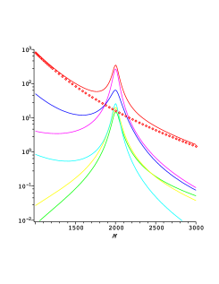
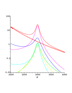
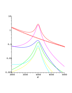
Figure 1: Invariant mass distributions $d\sigma/dM$ [fb/GeV] for the case of $M_{s}=2,3,4$ TeV from left to right. The correspondence of the colored line to the processes as, blue: $gg\rightarrow gg$, magenta: $qg\rightarrow qg$, cyan: ${\bar{q}}g\rightarrow{\bar{q}}g$, yellow: $gg\rightarrow q{\bar{q}}$, green: $q{\bar{q}}\rightarrow gg$, red: QCD background plus string resonances, and red points: QCD background.

3 Angular analysis of dijet events

It is natural to consider angular distribution of dijets to reveal that resonance structure in dijet invariant mass distribution consists many states with different spins. We consider $\chi\equiv\exp(2y)$ distributions with $M^{2}$ integrated over some certain ranges (see [10] and references therein). The $\chi$-distribution is defined from eq.(12) as

$${{d\sigma_{ij\rightarrow kl}}\over{d\chi}}=\int_{M^{2}_{\rm low}}^{M^{2}_{\rm high}}dM^{2}\int_{-Y_{max}}^{Y_{max}}dY\ x_{1}f_{i}(x_{1},M^{2})\ x_{2}f_{j}(x_{2},M^{2})\ {1\over{(1+\chi)^{2}}}\cdot{{d\sigma_{ij\rightarrow kl}}\over{d\hat{t}}}.$$ (16)

In the following we take $Y_{\rm max}=1$ and $1<\chi<20$ which corresponds to $0<y<1.5$ (and $\sqrt{s}=14$ TeV). We consider two kinds of integration regions on $M^{2}$:

$$M^{2}_{\rm low}=(M_{s}-250\,\mbox{GeV})^{2},\quad M^{2}_{\rm high}=(M_{s}+250\,\mbox{GeV})^{2}\qquad\mbox{: ``on peak''}$$ (17)

$$M^{2}_{\rm low}=(M_{s}-750\,\mbox{GeV})^{2},\quad M^{2}_{\rm high}=(M_{s}-250\,\mbox{GeV})^{2}\qquad\mbox{: ``off peak''}$$ (18)

As shown in Fig.1 $qg\rightarrow qg$ process dominates for “on peak” case in any value of $M_{s}=2,3$ and $4$. It is also true for “off peak” case except for the case of $M_{s}=2$, where $gg\rightarrow gg$ process dominates.

Fig.2 show individual contributions of six processes to “on peak” $\chi$-distribution and Fig.3 show the same for “off peak” case. It is expected that the distribution of QCD background is almost flat, and large values at small $\chi$ indicate “new physics” (for detail see Ref.[13], for example). Fig.2 includes very roughly estimated QCD backgrounds. For “off peak” case QCD background is very large: about $29000$ [fb], $1600$ [fb] and $150$ [fb] for $M_{s}=2,3$ and $4$ TeV, respectively. In case of “on peak” the process of $qg\rightarrow qg$ always dominates and other processes are negligible at large values of $M_{s}\gtrsim 4$ TeV. In case of “off peak” the process of $gg\rightarrow gg$ dominates at small value of $M_{s}\sim 2$ TeV due to the effect of gluon parton distribution function. At higher value of $M_{s}>3$, the process of $qg\rightarrow qg$ dominates the others also in “off peak” case.

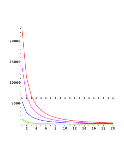
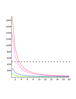
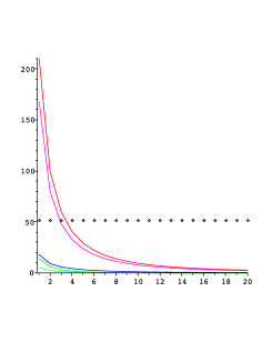
Figure 2: “on peak” $\chi$-distributions $d\sigma/d\chi$ [fb] for the case of $M_{s}=2,3$ and $4$ TeV from left to right. The color mapping to six processes are the same in Fig.1 except for that red line indicates total distribution. Black dots indicate rough estimates of QCD backgrounds.

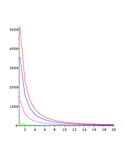
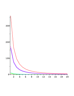
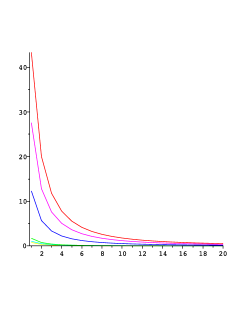
Figure 3: “off peak” $\chi$-distributions $d\sigma/d\chi$ [fb] for the case of $M_{s}=2,3$ and $4$ TeV from left to right. The color mapping to six processes are the same in Fig.1 except for that red line indicates total distribution.

Six processes predict the following form of $\chi$-distributions.

$${1\over{(1+\chi)^{2}}}\left(A_{1}+B_{1}\ {{1+\chi^{4}}\over{(1+\chi)^{4}}}\right)\quad\mbox{for $gg\rightarrow gg$},$$ (19)

$${1\over{(1+\chi)^{2}}}\left(A_{2}+B_{2}\ {{1+\chi^{3}}\over{(1+\chi)^{3}}}\right)\quad\mbox{for $qg\rightarrow qg$ and ${\bar{q}}g\rightarrow{\bar{q}}g$},$$ (20)

$${1\over{(1+\chi)^{2}}}\ B_{3}\ {{\chi(1+\chi^{3})}\over{(1+\chi)^{4}}}\quad\mbox{for $gg\rightarrow q{\bar{q}}$ and $q{\bar{q}}\rightarrow gg$},$$ (21)

where $A_{1},A_{2},B_{1},B_{2}$ and $B_{3}$ are constants. The common factor $1/(1+\chi)^{2}$ is a kinematical one in eq.(16). The first distribution, eq.(19), indicates a combination of spin $0$ and spin $2$ intermediate states with two massless spin $1$ gluons as initial states. The second distribution, eq.(20), indicates a combination of spin $1/2$ and $3/2$ intermediate states with initial state of one massless spin $1/2$ quark (or anti-quark) and one massless spin $1$ gluon. The third distribution, eq.(21), indicates a spin $1$ state in spin $2$ intermediate state, where massless quark and anti-quark couple with a spin $1$ state.

Fig.4 show various fits of “on peak” $\chi$-distribution in case of $M_{s}=2$ TeV with eq.(20). Since the process $qg\rightarrow qg$ dominates “on peak” distributions, it should be fit well with both non-vanishing $A_{2}$ and $B_{2}$. This is true as it is shown in the first figure in Fig.4. If this fit is better than that the other two fits, assuming only spin $3/2$ intermediate state or only spin $1/2$ intermediate state, we see that at least two degenerate states contribute, which is the prediction of string models. The second and the third figures in Fig.4 show the fits assuming single intermediate state. We see that two-state fit is better than single state fit. Since the actual situation depends on experimental precision and uncertainties, the feasibility of this procedure should be considered with detector simulations. Subtraction of QCD background is also a crucial issue.

It would be very difficult to distinguish small difference between eq.(19) and eq.(20) experimentally. Even though the process $gg\rightarrow gg$ dominates “off peak” distribution with $M_{s}=2$ TeV, the goodness of fit with eq.(19) and that with eq.(20) are almost the same. If we could separate gluon jets and quark jets with a certain efficiency, investigating both “on peak” and ‘off peak” distributions could be meaningful.

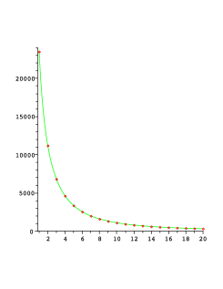
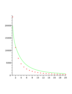
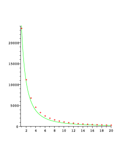
Figure 4: Three fits for “on peak” $\chi$-distribution ($M_{s}=2$ TeV) with eq.(20). Red points indicate the distribution by string excited stets and green lines indicate fit lines. From left to right, fit with $A_{2},B_{2}\neq 0$ (both spin $1/2$ and $3/2$ intermediate states), fit with $A_{2}=0$ (only spin $3/2$ intermediate state) and fit with $B_{2}=0$ (only spin $1/2$ intermediate state).

4 Effects of the mass shift in gluon dijet events

If it is possible to distinguish gluon jets and quark jets in a certain efficiency, it may be possible to investigate the process $gg\rightarrow gg$ independently. This is an interesting process with contributions of four string excited states as we can see in eq.(1). Though two color octet states obtain small one-loop correction to their masses, the masses of two color singlet states may obtain large one-loop corrections. It is shown in ref.[14] by explicit calculations in string world-sheet theory that anomalous U$(1)$ gauge boson, which is massless at tree level, obtain mass of the order of $0.1\times M_{s}^{2}$ or larger through the open string one-loop effect, or through the tree-level mixing with closed string states. The same may happen for the states $C^{*}_{J=0}$ and $C^{*}_{J=2}$. In the next section, we will estimate the shift of mass squared of $C^{*}_{J=2}$ is $\Delta m^{2}=(3/\pi^{3})M_{s}^{2}$ by explicit calculations. Namely, the shift of mass squared of $C^{*}_{J=2}$ (and $C^{*}_{J=0}$) is of the order of $10\%$ of $M_{s}^{2}$. This gives a non-trivial shape to resonance structure by the process $gg\rightarrow gg$.

Fig.5 show parton-level total cross sections of the process $gg\rightarrow gg$ with mass shifts. We see that the shape of simple Breit-Wigner type resonance is largely distorted especially for larger value of $M_{s}$. In real observable, dijet invariant mass distributions, this distortion is smeared as shown in Fig.6 (with rapidity cut $|y_{1}|$, $|y_{2}|<1$ and $\sqrt{s}=14$ TeV). We see that the value of the left of the peak decreases and the value of the right of the peak increases by the effect of mass shifts.

In actual experiments, we can not escape from the contamination due to dominant process $qg\rightarrow qg$, even if a certain level of gluon jets selection might be possible. Fig.7 show dijet invariant mass distributions including the process $qg\rightarrow qg$ with reduction of $1/3$ and the process $gg\rightarrow gg$ with reduction of $2/3$. Assuming the subtraction of QCD background, we can consider the following ratio of cumulative cross sections as a measure of the existence of mass shifts or distortion from simple Breit-Wigner type shape.

$$R\equiv{{\sigma_{\rm left}-\sigma_{\rm right}}\over{\sigma_{\rm left}+\sigma_{\rm right}}},$$ (22)

where

$$\sigma_{\rm left}\equiv\int_{M_{s}-\Delta M}^{M_{s}}dM{{d\sigma}\over{dM}},\qquad\sigma_{\rm right}\equiv\int_{M_{s}}^{M_{s}+\Delta M}dM{{d\sigma}\over{dM}}.$$ (23)

The values of this ratio in case of $\Delta M=1000$ GeV are

$$R_{\Delta m^{2}\neq 0}\simeq 0.26,\quad R_{\Delta m^{2}=0}\simeq 0.31\quad(R_{\Delta m^{2}\neq 0}/R_{\Delta^{2}=0}\simeq 0.83)\quad\mbox{for $M_{s}=2$ TeV},$$ (24)

$$R_{\Delta m^{2}\neq 0}\simeq 0.18,\quad R_{\Delta m^{2}=0}\simeq 0.22\quad(R_{\Delta m^{2}\neq 0}/R_{\Delta^{2}=0}\simeq 0.80)\quad\mbox{for $M_{s}=3$ TeV},$$ (25)

$$R_{\Delta m^{2}\neq 0}\simeq 0.19,\quad R_{\Delta m^{2}=0}\simeq 0.22\quad(R_{\Delta m^{2}\neq 0}/R_{\Delta^{2}=0}\simeq 0.85)\quad\mbox{for $M_{s}=4$ TeV}.$$ (26)

The number of events ${\cal L}\sigma_{\rm left}$ with ${\cal L}=100\ {\rm fb}^{-1}$ are of the order of $10^{5}$, $10^{4}$ and $10^{3}$ for $M_{s}=2,3$ and $4$ TeV, respectively. In case of small $M_{s}\sim 2$ TeV, the selection of gluon jets is not so crucial, since the process $gg\rightarrow gg$ dominates in left region. In case of larger $M_{s}$ the selection becomes more important. The precise determination of QCD background is very important not to generate systematic unbalance in left and right regions by the subtraction.

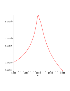
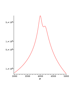
Figure 5: Total cross sections (unit [fb]) of the process $gg\rightarrow gg$ in ideal (unrealistic) gluon-gluon collider scanning $M=\sqrt{\hat{s}}$. From left to right, $M_{s}=2,3$ and $4$ TeV.

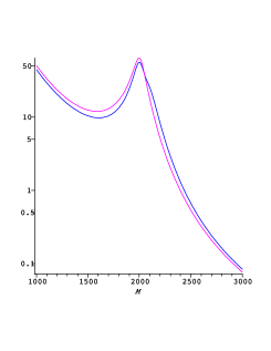
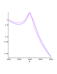
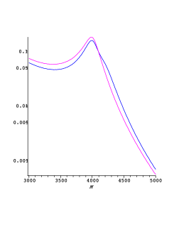
Figure 6: Dijet invariant mass distributions (unit [fb/GeV]) of the process $gg\rightarrow gg$ without QCD background. The line with color blue is that with mass shifts and the line with color magenta is that without mass shifts. From left to right, $M_{s}=2,3$ and $4$ TeV.

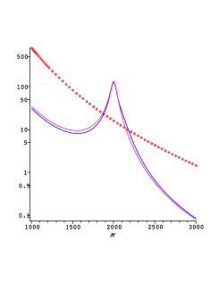
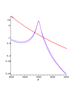
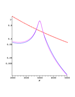
Figure 7: Dijet invariant mass distribution of the process $gg\rightarrow gg$ plus $qg\rightarrow qg$ (unit [fb/GeV]). The line with color blue is that with mass shifts and the line with color magenta is that without mass shifts. The points with red denote QCD backgrounds. From left to right, $M_{s}=2,3,4$ TeV.

5 Calculation of the mass shift in String Theory

The one-loop corrections to the masses of first string excited states can be calculated in string world-sheet theory. We calculate one-loop mass correction to the state $C^{*}_{J=2}$ by investigating its two point amplitude along the line of ref.[14] in which one-loop mass of anomalous U$(1)$ gauge boson is explicitly calculated. It is assumed that color gauge symmetry is on a stack of D3-brane. The two point amplitude of $C^{*}_{J=2}$ can be written as follows.

$$A_{2}=\int_{0}^{\infty}{{dt}\over{2t}}\int_{0}^{t}dx\ \langle V_{1}(z_{1})V_{2}(z_{2})\rangle_{t},$$ (27)

where $z_{1}=\exp(-x)$ and $z_{2}=\exp(i\pi)$, and $\langle\cdots\rangle_{t}$ denotes correlation functions on cylinder with modulus $t$. The operators $V_{1}(z_{1})$ and $V_{2}(z_{2})$ are vertex operators with picture $0$ of $C^{*}_{J=2}$ with momenta $k_{1}$ and $k_{2}$ (both incoming) and polarizations $e^{(1)}_{\mu\nu}$ and $e^{(2)}_{\mu\nu}$ (traceless antisymmetric, and $k^{\mu}e_{\mu\nu}=0$) in four dimensional spacetime.

$$V_{1}(z_{1}) = {1\over\sqrt{2\alpha^{\prime}}}\ T_{C^{*}_{J=2}}\ e^{(1)}_{\mu\nu}\left\{i\partial X^{\mu}i\partial X^{\nu}+2\alpha^{\prime}\left((k_{1}\cdot\psi)i\partial X^{\mu}\psi^{\nu}+\partial\psi^{\mu}\psi^{\nu}\right)\right\}e^{ik_{1}\cdot X},$$ (28)

$$V_{2}(z_{2}) = {1\over\sqrt{2\alpha^{\prime}}}\ T_{C^{*}_{J=2}}\ e^{(2)}_{\mu\nu}\left\{i\partial X^{\mu}i\partial X^{\nu}+2\alpha^{\prime}\left((k_{2}\cdot\psi)i\partial X^{\mu}\psi^{\nu}+\partial\psi^{\mu}\psi^{\nu}\right)\right\}e^{ik_{2}\cdot X},$$ (29)

where $T_{C^{*}_{J=2}}={\rm diag}(1/\sqrt{6},1/\sqrt{6},1/\sqrt{6})$ is Chan-Paton matrix for the state $C^{*}_{J=2}$. We consider only the non-planar diagram, which include the effect of mixing between closed string states and open string states.

The amplitude can be explicitly written as follows.

$$A_{2} = ({\rm tr}(T_{C^{*}_{J=2}}))^{2}\ {1\over{2\alpha^{\prime}}}\int_{0}^{\infty}{{dt}\over{2t}}\int_{0}^{t}dx\ 2\ e^{(1)}_{\mu\nu}e^{(2)}{}^{\mu\nu}\ {1\over 2}\sum_{\alpha,\beta=0,1}(-1)^{\alpha}\langle e^{ik_{1}\cdot X}e^{ik_{2}\cdot X}\rangle$$ (30)

$$\qquad\times\Bigg{\{}(2\alpha^{\prime})^{2}\langle\partial\psi\psi\rangle\langle\psi\partial\psi\rangle+\langle\psi\psi\rangle^{2}\langle\partial XX\rangle\langle X\partial X\rangle\Bigg{\}}Z^{\alpha\beta}(t),$$

where

$$(2\alpha^{\prime})^{2}\langle\partial\psi\psi\rangle\langle\psi\partial\psi\rangle = {{(2\alpha^{\prime})^{2}}\over{8z_{1}}}\cdot{{({\cal P}^{\prime}(z_{1}+1))^{2}}\over{{\cal P}(z_{1}+1)+4\pi i\partial_{\tau}\ln\left(\theta\left[\begin{array}[]{c}\alpha/2\\ \beta/2\end{array}\right](0|\tau)\bigg{/}\eta(\tau)\right)}}$$ (33)

$$\langle\psi\psi\rangle^{2}\langle\partial XX\rangle\langle X\partial X\rangle = -2\pi i\partial_{\tau}\ln\left(\theta\left[\begin{array}[]{c}\alpha/2\\ \beta/2\end{array}\right](0|\tau)\Big{/}\eta(\tau)\right)$$

$$\times{1\over{z_{1}}}\left({{\alpha^{\prime}}\over{2\pi}}\right)^{2}\left\{{{\theta_{1}^{\prime}((ix-\pi)/2\pi|\tau)}\over{\theta_{1}((ix-\pi)/2\pi|\tau)}}-{{ix}\over{\tau_{2}}}\right\}\left\{{{\theta_{1}^{\prime}((\pi-ix)/2\pi|\tau)}\over{\theta_{1}((\pi-ix)/2\pi|\tau)}}+{{ix}\over{\tau_{2}}}\right\},$$

$$\langle e^{ik_{1}\cdot X}e^{ik_{2}\cdot X}\rangle = \left({{2\pi(\eta(\tau))^{3}}\over{\theta_{2}(ix/2\pi|\tau)}}e^{{\pi\over{(2\pi)^{2}}}{{x^{2}}\over{\tau_{2}}}}\right)^{2\alpha^{\prime}k_{1}\cdot k_{2}},$$ (37)

and

$$Z^{\alpha\beta}(t)=(-1)^{(1-\alpha)\beta}{{iV_{4}}\over{(\sqrt{8\pi^{2}\alpha^{\prime}t})^{4}}}{1\over{(\eta(\tau))^{8}}}\left(\theta\left[\begin{array}[]{c}\alpha/2\\ \beta/2\end{array}\right](0|\tau)\Big{/}\eta(\tau)\right)^{4}.$$ (38)

Here, $\tau=\tau_{1}+i\tau_{2}$ with $\tau_{1}=0$ and $\tau_{2}=t$, $V_{4}$ is the volume of four dimensional spacetime, ${\cal P}$ is the Weierstrass function and ${\cal P}^{\prime}$ is its derivative, $\eta(\tau)$ is the Dedekind function, and

$$\theta\left[\begin{array}[]{c}a\\ b\end{array}\right](z|\tau)\equiv e^{2\pi ia(z+b)}q^{a^{2}/2}\prod_{n=1}^{\infty}(1-q^{n})\prod_{m=1}^{\infty}(1+q^{m+a-1/2}e^{2\pi i(z+b)})(1+q^{m-a-1/2}e^{-2\pi i(z+b)})$$ (39)

is the $\theta$-function ($q=e^{2\pi i\tau}$) with $\theta_{1}(z|\tau)$ is the case of $a=b=1/2$ and $\theta_{1}^{\prime}(z|\tau)=\partial\theta_{1}(z|\tau)/\partial z$, and $\theta_{2}(z|\tau)$ is the case of $a=1/2$, $b=0$.

We can go from open string one-loop picture to closed string tree picture by changing modulus variable from $t$ to $s=\pi/t$ and doing modular transformation. As an order estimate, we consider the asymptotic form in the limit of $s\rightarrow\infty$. Then the two point amplitude becomes

$$A_{2}\sim-iV_{4}\ {1\over 4}e^{(1)}_{\mu\nu}e^{(2)}{}^{\mu\nu}\ ({\rm tr}(T_{C^{*}_{J=2}}))^{2}{1\over{2\alpha^{\prime}}}{{16}\over{(4\pi)^{3}}}\int_{0}^{\infty}ds\ s^{2}\ e^{-s/2}.$$ (40)

The relations $k_{2}=-k_{1}$ and $k_{1}\cdot k_{1}=-1/\alpha^{\prime}=-M_{s}^{2}$ (with different metric signature from that in previous sections) have been used. The factor $e^{-s/2}$ comes from eq.(37) indicating tree level propagation of massive closed string states. Then the order of the mass shift becomes

$$\Delta m^{2}\sim({\rm tr}(T_{C^{*}_{J=2}}))^{2}{1\over{2\alpha^{\prime}}}{{16}\over{(4\pi)^{3}}}\int_{0}^{\infty}ds\ s^{2}\ e^{-s/2}={3\over{\pi^{3}}}M_{s}^{2}.$$ (41)

This result means that the mass shift about $10\%$ of $M_{s}^{2}$ is expected for color singlet open string states $C^{*}_{J=2}$ (and $C^{*}_{J=0}$).

6 Conclusions

It has been stressed that a distinguished point of low-scale string models from the other “new physics”, like quark compositeness, on the resonance in dijet invariant mass distribution is that a resonance consists many resonances by many degenerate intermediate states with different spins. Therefore, to discover or exclude low-scale string models, it is very important to find the procedures to see the “structure” of resonance.

It has been proposed two procedures. One is the analysis of angular distributions ($\chi$-distributions), and the other is looking for the distortion of the resonance shape due to the mass shifts in string excited states. Further detailed analysis including detector simulation is necessary to clarify real feasibility of these procedures at the LHC.

The center of mass energy of $pp$ collision $\sqrt{s}=14$ TeV has been assumed in all the analysis in previous sections. It is planned that the LHC will operate at $\sqrt{s}=7$ TeV until obtaining integrated luminosity $1\,{\rm fb}^{-1}$. In Fig.8 three plots assuming $\sqrt{s}=7$ TeV for the case $M_{s}=2$ TeV are given. In view of the number of events, the feasibility of the analysis seems to be similar to the case of $M_{s}=3$ TeV with $\sqrt{s}=14$ TeV.

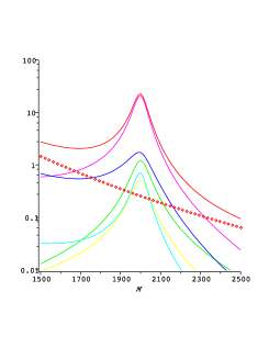
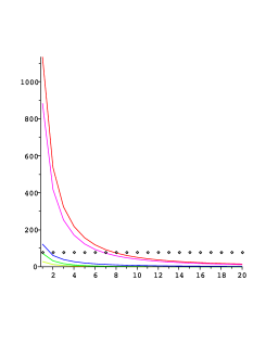
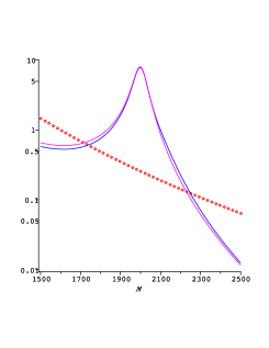
Figure 8: Plots in case of center of mass energy $7$ TeV. From left to right, dijet invariant mass distribution (the same plot of Fig.1), “on peak”$\chi$-distribution (the same plot of Fig.2), and dijet invariant mass distribution with mass shift (the same plot of Fig.7).

References

- [1] I. Antoniadis, “A Possible new dimension at a few TeV,” Phys. Lett. B 246 (1990) 377.
- [2] I. Antoniadis, “String physics at low energies,” Prog. Theor. Phys. Suppl. 152 (2004) 1.
- [3] I. Antoniadis, “Topics on String Phenomenology,” arXiv:0710.4267 [hep-th].
- [4] I. Antoniadis, K. Benakli and M. Quiros, “Radiative symmetry breaking in brane models,” Nucl. Phys. B 583 (2000) 35 [arXiv:hep-ph/0004091].
- [5] N. Kitazawa, “Radiative symmetry breaking on D-branes at non-supersymmetric singularities,” Nucl. Phys. B 755 (2006) 254 [arXiv:hep-th/0606182].
- [6] S. Cullen, M. Perelstein and M. E. Peskin, “TeV strings and collider probes of large extra dimensions,” Phys. Rev. D 62 (2000) 055012 [arXiv:hep-ph/0001166].
- [7] L. A. Anchordoqui, H. Goldberg, D. Lust, S. Nawata, S. Stieberger and T. R. Taylor, “Dijet signals for low mass strings at the LHC,” Phys. Rev. Lett. 101 (2008) 241803 [arXiv:0808.0497 [hep-ph]].
- [8] L. A. Anchordoqui, H. Goldberg and T. R. Taylor, “Decay widths of lowest massive Regge excitations of open strings,” Phys. Lett. B 668 (2008) 373 [arXiv:0806.3420 [hep-ph]].
- [9] L. A. Anchordoqui, H. Goldberg, D. Lust, S. Nawata, S. Stieberger and T. R. Taylor, “LHC Phenomenology for String Hunters,” Nucl. Phys. B 821 (2009) 181 [arXiv:0904.3547 [hep-ph]].
- [10] T. Nunnemann [D0 Collaboration and CDF Collaboration], “Searches for leptoquark production and compositeness at the Tevatron,” PoS E PS-HEP2009 (2009) 268 [arXiv:0909.2507 [hep-ex]].
- [11] D. Lust, S. Stieberger and T. R. Taylor, “The LHC String Hunter’s Companion,” Nucl. Phys. B 808 (2009) 1 [arXiv:0807.3333 [hep-th]].
- [12] J. Pumplin, D. R. Stump, J. Huston, H. L. Lai, P. M. Nadolsky and W. K. Tung, “New generation of parton distributions with uncertainties from global QCD analysis,” JHEP 0207 (2002) 012 [arXiv:hep-ph/0201195].
- [13] N. Boelaert and T. Akesson, “Dijet angular distributions at TeV,” Eur. Phys. J. C 66 (2010) 343 [arXiv:0905.3961 [hep-ph]].
- [14] I. Antoniadis, E. Kiritsis and J. Rizos, “Anomalous U(1)s in type I superstring vacua,” Nucl. Phys. B 637 (2002) 92 [arXiv:hep-th/0204153].