Performance of XFaster likelihood in real CMB experiments
Abstract
We assess the strengths and weaknesses of several likelihood formalisms, including the XFaster likelihood. We compare the performance of the XFaster likelihood to that of the Offset Lognormal Bandpower likelihood on simulated data for the Planck satellite. Parameters estimated with these two likelihoods are in good agreement. The advantages of the XFaster likelihood can therefore be realized without compromising performance.
keywords:
Cosmology: observations – methods: data analysis – cosmic microwave background1 Introduction
The temperature and polarization anisotropies of the Cosmic Microwave Background (CMB) contain a wealth of cosmological information. In extracting this information from measurements of the CMB, the likelihood function , where is the theoretical spectrum for some cosmological model, plays an important role. For Gaussian fluctuations, is given by a Multivariate Gaussian of the observed data (section 2). For low resolution data (, defined more precisely later) in the usual spherical harmonic expansion, it is computationally feasible to evaluate this directly. For high resolution data, it is not, and computationally tractable approximations are required. Fortunately, the large number of independent samples of the universe at high resolution, coupled with a much more nearly diagonal covariance matrix, mean that approximations exist that are accurate as well as fast. The subject of this paper is the performance of one such high method, the “XFaster likelihood.”
A successful high method must account correctly for correlations induced in the angular power spectra by partial sky coverage, non-uniform noise, and non-zero beamwidths, as well as the temperature and polarization cross power. A number of approaches for high- have been proposed. For temperature alone, these include the Gaussian, Offset Lognormal, Equal Variance (Bond, Jaffe, & Knox 2000), WMAP (Verde et al. 2003), and SCR (Smith, Challinor, & Rocha 2006) likelihood approximations. For temperature and polarization together, these include the Offset Lognormal Bandpower, Hamimeche and Lewis (Hamimeche & Lewis 2008), and XFaster (Rocha et al. 2009) likelihoods.
This paper is organized as follows. In Section 2 we describe the the Multivariate Gaussian likelihood both in pixel and harmonic space, give an overview of existing high approximations (Section 2.2) and their limitations. An account of their performances applied to simulated Planck data has been given in (Rocha et al. 2009). We further test the performance of XFaster likelihood implemented in a new, modified version of the publicly available software CosmoMC code111http://cosmologist.info/cosmomc/ (Lewis and Bridle (2002)) by applying it to estimation of cosmological parameters, and compare it to the Offset Lognormal Bandpower likelihood. We further test our approach to tackle the asymmetry of the beams by comparing parameters estimated for Planck simulated data convolved with a symmetric and a asymmetric beam using both likelihood approaches.
2 Likelihood for a Gaussian sky
Pixel temperature fluctuations (Stokes ) on the celestial sphere can be expanded in terms of spherical harmonics as
| (1) |
with coefficients . Polarization fluctuations (Stokes and ) can be expanded in spin-2 spherical harmonics, , with and (grad- or curl-type) polarization coefficients
| (2) |
If the CMB is a Gaussian isotropic field, then the probability of a measurement of the sky given a model is described by a Multivariate Gaussian of the observed data:
| (3) |
where is the covariance of the data , and is the set of model parameters. , where is the sky signal and is the noise. Since measurements of the sky are pixelated, the above likelihood is often called the ”pixel-based likelihood” when estimated in the pixel domain. It can be evaluated directly if the number of pixels is not too large, but for a full-sky experiment such as Planck with 5′ pixels it is impossible with current computers.
2.1 Exact likelihood in harmonic space
If the CMB is Gaussian, its statistical properties are represented fully by the underlying power spectrum . The multipole harmonic coefficients, (where is , , or ), on different scales are independent of one another, and we can write
| (4) |
The are complex. Under the assumption of Gaussianity, their real and imaginary parts are independent and Gaussian distributed, hence their phases are random. Since the CMB is real, they must satisfy . This means that is real.
For we have
| (5) |
For , we have for the real part of the
| (6) |
where
| (7) |
and
| (8) |
Similarly for the imaginary part.
Combining together all the values of , we find, for a particular :
| (9) |
where
| (10) |
and the normalisation is independent of and . In data analysis, the measured power spectrum is a fixed quantity, hence the dependence of the likelihood on this value is generally dropped. In this case, up to a constant, we can write the log-likelihood as
| (11) |
i.e., the inverse Wishart distribution. If we consider only one measurement, e.g., one -mode or -mode, we can write the likelihood function as (Bond, Jaffe, & Knox 2000)
| (12) |
i.e., the inverse Gamma distribution, where is the theoretical value of (or ) and is the measured value.
We can write an exact expression for the likelihood function for our measured power spectrum given the true underlying power spectrum , which is a function of cosmological parameters. Since this likelihood is usually considered in the context of data analysis, it is common to regard the measured as fixed quantities, and to write the likelihood as
| (13) |
where the constant depends on . For fixed , this function peaks at . However if we wish to consider the likelihood as a function of then it is necessary to include the -dependence of the likelihood, in which case it should be written as
| (14) |
For a fixed underlying power spectrum , this function peaks at .
This is adequate for a full-sky experiment with an infinitely narrow beam and no instrumental noise. For a partial or “cut” sky it is necessary to account for the correlations between the that are introduced. In addition, real experiments always have non-uniform noise, and must estimate bandpowers () rather than individual . We need to find an appropriate likelihood function that includes the correct correlations and accounts properly for noise.
2.2 Approximating the likelihood at high-
Although the signal and the noise can be assumed Gaussian, the distribution of the band powers is non-Gaussian. This is the so called ’cosmic bias’—the distribution is skewed towards higher values. This effect is most noticeable at low where cosmic variance of the signal dominates the error bars. As we will see, the full likelihood includes the cosmic bias whereas the Gaussian approximation of the Fisher matrix does not. The Joint likelihood for temperature and polarization carries an extra complication in that one has to find an approximation that properly accounts for the temperature and polarization cross power. We will start by considering the current approximations derived for temperature alone, followed by an account on existing attempts to extend it to a joint likelihood for temperature and polarization.
2.2.1 Temperature only
Gaussian Likelihood—The first level of approximation is to use a likelihood that is Gaussian in the (Bond, Jaffe, & Knox 2000), i.e.,
| (15) |
where is a vector of values (and similarly ) and is the inverse signal covariance matrix. However this likelihood function is well-known to be biased, (see e.g., Bond, Jaffe, & Knox (2000); Smith, Challinor, & Rocha (2006)). This Gaussian likelihood can be implemented in two ways. The version discussed in Bond, Jaffe, & Knox (2000) considers the case where the signal covariance matrix is derived from the measured power spectrum, rather than the theoretical power spectrum. This results in an overestimation of the errors if the measured power spectrum has fluctuated upwards, and hence upward fluctuations are given less weight, leading to an overall downward bias. The covariance matrix can instead be computed from the theoretical power spectrum, as used in Verde et al. (2003), leading to an overestimation of the amplitude.
Offset Lognormal Likelihood—A better approximation to the likelihood is the Offset Lognormal approximation (Bond, Jaffe, & Knox 2000), given by
| (16) |
where and the matrix is related to the inverse covariance matrix by
| (17) |
(The offset factors are simply a function of the noise and beam of the experiment.) This likelihood function is still slightly biased, but in the opposite direction to that of the Gaussian likelihood.
To some extent the Offset Lognormal approximation addresses this issue, in that the transformation of variables from to has a constant curvature matrix. Hence the uncertainties on the do not depend on the , avoiding the cosmic bias. To proceed, assume a normal distribution in this new variable instead of . The likelihood is now closer to the exact one. Nevertheless, there is still a small bias opposite to that introduced by the Gaussian approximation in .
WMAP Likelihood—Taking advantage of the fact that the bias for the Offset Lognormal likelihood is opposite to that introduced by the Gaussian likelihood, the WMAP team defined a likelihood that is a weighted combination of the two (Verde et al. 2003):
| (18) |
This likelihood is a significantly better approximation for the case of a Gaussian CMB. However, the fact that a likelihood function is accurate in the absence of correlations (when the probability of a measured power spectrum is purely a function of the input power spectrum rather than having any additional dependence on the cosmology) is not a guarantee that it will perform well when applied to a non-Gaussian sky. For instance, Smith, Challinor, & Rocha (2006) have shown that the WMAP likelihood gives significant biases in the dark energy parameter, , when considering the lensed B-mode power spectrum.
Equal Variance Likelihood—The equal variance likelihood proposed by Bond, Jaffe, & Knox (2000) is given by:
| (19) |
with
| (20) |
and
| (21) |
The noise offset is estimated using the equation of the maximum likelihood solution for the , replacing the observed map with the average of the noise Monte Carlo simulation power spectra .
SCR Likelihood—Smith, Challinor, & Rocha (2006) developed a new likelihood to tackle the non-Gaussianity of the lensed sky for studies of the -mode power spectrum; however, this likelihood has not been extended to the joint probability distribution for all modes. By considering the curvature (with respect to the measured ) of the exact log-likelihood expression for a Gaussian sky (equation 14) at its peak, and also the third derivative, a new likelihood can be derived which is Gaussian in , where both the second and third derivatives with respect to take the correct values at the peak of the likelihood.
The SCR likelihood approximates the normalised distribution as Gaussian in some function of the , and takes the form
| (22) |
where
| (23) | |||||
| (24) |
and
| (25) |
Here is the covariance matrix of the measured at parameters . The normalisation is
| (26) |
which can be approximated by .
Applying this expression to a Gaussian simulation gives results almost indistinguishable from the exact likelihood expression, as shown in Smith, Challinor, & Rocha (2006). Ignoring the factors, however, is a bad approximation at low , since it ignores the fact that, for a fixed , the peak of the likelihood is slightly below . This ends up translating to an underestimation of the theoretical power spectrum. The performance of the Gaussian, WMAP, and two versions of the SCR likelihoods on full-sky lensed simulations was compared in Smith, Challinor, & Rocha (2006). The WMAP likelihood function gives very different results to the new SCR likelihood function, and shows a significant bias in the dark energy parameter, .
2.2.2 Temperature + polarization
We cannot merely extend the above approximations to build a joint likelihood for temperature and polarization. For instance, assume that we approximate the likelihood for as a Gaussian. The mode and variance of the Gaussian distribution for depend on and . Hence it is not enough to consider the joint likelihood as a product of independent , , and likelihoods. Indeed the trick is to find a way of coupling these components reliably. Furthermore, given that the power spectrum is at times negative, we cannot build a Joint likelihood as a product of independent Offset Lognormal likelihoods. As a quick fix, one could try the following:
Offset Lognormal Bandpower Likelihood—This likelihood is a joint likelihood for temperature and polarization built as a Gaussian for and Offset Lognormal for , , and . However, this approximation does not properly take into account temperature and polarization cross power.
The following two likelihoods, the Hamimeche and Lewis and XFaster likelihoods, do attempt to take temperature and polarization cross power into account properly.
Hamimeche and Lewis (HL) Likelihood—The Hamimeche & Lewis (2008) likelihood generalizes the full-sky exact likelihood given by Equation 11 to the cut sky by considering a quadratic expression of the form
| (27) |
where and . This approximation involves a fiducial model so that the covariance can be pre-computed. It is assumed that the matrix of estimators is positive/definite, although this assumption may break down for some estimators at low-.
XFaster Likelihood—The XFaster likelihood, introduced in Contaldi et al. (2009) and Rocha et al. (2009), takes the following form for temperature alone:
| (28) |
where a tilde connotes a quantity estimated on the cut-sky. The power spectrum is parameterized through a set of deviations from a template full-sky spectrum ,
| (29) |
where is the coupling matrix due to the cut sky observations, expresses the effect of a finite beam, and is a transfer or filter function accounting for the effect of pre-filtering the data in both time and spatial domains.
Extending to polarization, we have
| (30) |
where the matrix is block diagonal: , with each multipole’s covariance given by the matrix
| (31) |
This likelihood follows intuitively from the full-sky exact likelihood, the Inverse Wishart distribution, as given by Equation 11.
2.3 The likelihood at low-
The pixel-based Multivariate Gaussian likelihood given by Equation 3 can be computed up to , and is adequate for comparison with Xfaster as shown in (Rocha et al. 2009). (Faster methods (see summary by Ashdown et al. (2010)) have been developed, but are not necessary here.) We use an implementation known as Bflike, described as follows.
A CMB map can be written as an ordered vector , comprising all pixels with valid observations. In general and the sets of indexes of temperature and polarization measurements will be different. Assuming that both CMB and noise fluctuations in each pixel are Gaussian-distributed with zero mean, the likelihood for has the functional form given in equation (1), where the covariance matrix has a block structure:
| (32) |
Correlations between, e.g., temperature measurements in pixels and can be written as:
| (33) |
are the ordinary Legendre polynomials, and is the angle between the centers of pixels and . Notice that the include the contribution of the beam and pixel window, i.e., , where is the theory power spectrum and and are the harmonic transform of the beam and window functions respectively. For uncorrelated noise, , where is the rms noise in pixel . In general, is a dense matrix. Similar expressions hold for correlations involving and (see e.g., Tegmark & de Oliveira-Costa (2001)). The choice of in Equation 33 depends on several factors, including the smoothing beam, the signal-to-noise ratio, and the pixelization scheme.
3 Comparing likelihoods
3.1 Simulations
To compare the performance of XFaster with other likelihood functions, we use simulations developed within the Planck CTP working group. Planck (Planck Blue Book 2005; Tauber et al. 2009) is a full-sky experiment covering frequencies from 30 to 857 GHz with beams ranging in size from 33′ to 5′. A full description of the simulations is given in Ashdown et al. (2010); Rocha et al. (2009). Practical considerations of computational resources having to do with the size of the time-ordered data (TOD), the number of pixels in the maps, and the number of multipoles that had to be calculated, dictated the choice of the 70 GHz channel for the simulations. Higher frequency channels have higher angular resolution and sensitivity, and will extend to smaller angular scales with reduced error bars. Recent increases in computational capability make it possible now to generate thousands of Monte Carlo simulations at the higher frequencies as well. Results will be presented in a future publication Rocha et al. (2010); Ashdown et al. (2010).
The 70 GHz simulations used here include the CMB, realistic detector noise, and noise induced by temperature fluctuations of the 20-K hydrogen sorption cooler. To mimic the sensitivity of combination of channels, as would be used for separation of foregrounds with real data, the white noise level was taken to be lower than that expected for the 70 GHz channel alone. The white noise per sample was 2025.8 K and the noise power spectrum had knee frequency 0.05 Hz and slope . The input sky signal used to generate the “observed map” was the CMB map derived from the Planck CMB reference sky available in222http://www.sissa.it/ planck/reference-sky/CMB/alms/alm-cmb-reference-template-microKthermodynamic-nside2048.fits which uses the WMAP 1-year up to to generate the CMB. In other words, the large scale structure of the observed map is a WMAP-constrained realization.
The TOD were generated using modules of the Planck simulator pipeline, LevelS (Reinecke et al. 2005). Maps were made from the simulated time-ordered data (TOD) using the destriping code Springtide (Poutanen 2005; Ashdown et al. 2007a, b, 2009; Ashdown 2009b). Where a sky cut was applied, it was made at the boundary where the total intensity of the diffuse foregrounds and point sources exceeded twice the CMB sigma. Pixels missing due to the scanning strategy were masked. The beams of the detectors have FWHMs of 13′–14′, so the maps were made with , corresponding to a pixel size of 3.′4. Two sets of maps were provided, one 12-detector map to be used in the auto-spectrum mode, and three 4-detector maps to be used in the cross-spectrum mode.
Two cases were considered. The first, called Phase 2a for historical reasons, assumed symmetric Gaussian beams with FWHM of 14′. The second, Phase 2b, assumed elliptical Gaussians fit to the central parts of realistic beams calculated by a full diffraction code for the Planck optical system.
One hundred Monte Carlo signal simulations were generated from the best fit WMAP + CBI + ACBAR CDM power spectrum333available in http://lambda.gsfc.nasa.gov/product/map/dr1/lcdm.cfm, with BB mode power set to zero. For the symmetric beam case the signal could be simulated in the map domain, while noise was generated in the time domain. For the asymmetric beam case, both signal and noise simulations were generated in the time domain.
The “low- dataset” of the Phase2 simulations was generated directly at . The procedure adopted ensured consistency between the low- and high- datasets used to test the XFaster power spectrum and likelihood estimator; however, the low- dataset lacks the artifacts connected to smoothing and degradation of higher resolution maps that will be present in the final Planck maps.
As pointed out in Rocha et al. (2009), since the large scale structure of the observed map is derived from real observations, i.e., a WMAP constrained realization, it is not necessarily consistent with the best-fit spectrum at low multipoles. This discrepancy is evident when comparing the cosmological parameters estimated with XFaster power spectrum and likelihood and the Offset Lognormal likelihood with the theoretical best fit parameters. The Monte Carlo simulations, however, are realizations of the first year WMAP+CBI+ACBAR best fit CDM power spectrum for Phases 2a and 2b, so such discrepancy is no longer present. Parameters estimated from these Monte Carlo simulations maps are shown to be close to the WMAP best fit parameters.
3.2 Comparisons
Rocha et al. (2009) (Figs. 14 and 15) showed that for and , all of the likelihood approximations described above except the Gaussian likelihood converge to the same form at multipoles above 10 or 20. For , however, the Gaussian and the Lognormal likelihood differs from the rest up to high . Rocha et al. (2009) (Fig. 17) also showed by comparing XFaster with the pixel-based likelihood code (BFlike) that a transition from low- to high- codes was appropriate for Planck in the range –
Here we assess the performance of the XFaster likelihood by comparing cosmological parameters obtained with the XFaster and the Offset Lognormal Bandpower (i.e., Offset Lognormal likelihood for , , , and Gaussian for ) likelihoods. XFaster computes the likelihood of a model passed to it by a modified version of the publicly available CosmoMC code444http://cosmologist.info/cosmomc/ (Lewis and Bridle (2002))) for cosmological parameter Markov Chain Monte Carlo estimations. There is no need for window functions or the band power spectrum itself. The inputs are the raw pseudo- of the observations plus the kernel and transfer function required by XFaster to relate the cut-sky pseudo- to the full-sky .
For the Offset Lognormal Bandpower likelihood, window functions are required that properly account for band power spectrum correlations. We used two different window functions, top hat (box) and Fisher-weighted (Rocha et al. 2009), written . For the sake of completeness we describe here how we derive . To construct (following Bond, Jaffe, & Knox (2000) and Rocha et al. (2009)) we define a logarithmic integral,
| (34) |
which is used to calculate the expectation values for the deviations (when a shape model, is considered), or bandpowers (when is assumed to be flat).
| (35) |
where is the band power window function, with . We define normalized window functions
| (36) |
using the fact that
| (37) |
to obtain
| (38) |
Extending to polarization:
| (39) |
where , and gives the cut-sky response to the individual full-sky multipoles,
| (40) |
The parameters calculated are: baryonic, cold dark matter, and cosmological constant densities, , , and , respectively; the ratio of the sound horizon to the angular diameter distance at decoupling, ; the spectral index of the initial fluctuation spectrum, ; the overall normalization of the spectrum at Mpc-1 (); the Hubble constant ; and the reionization redshift . We treat in two different ways. Rocha et al. (2009) showed that “high ” codes could be used to determine parameters from the “observed map” quite well if was fixed in the fit to the value of the input model. This works because is constrained primarily by data at . We indicate when is held fixed.
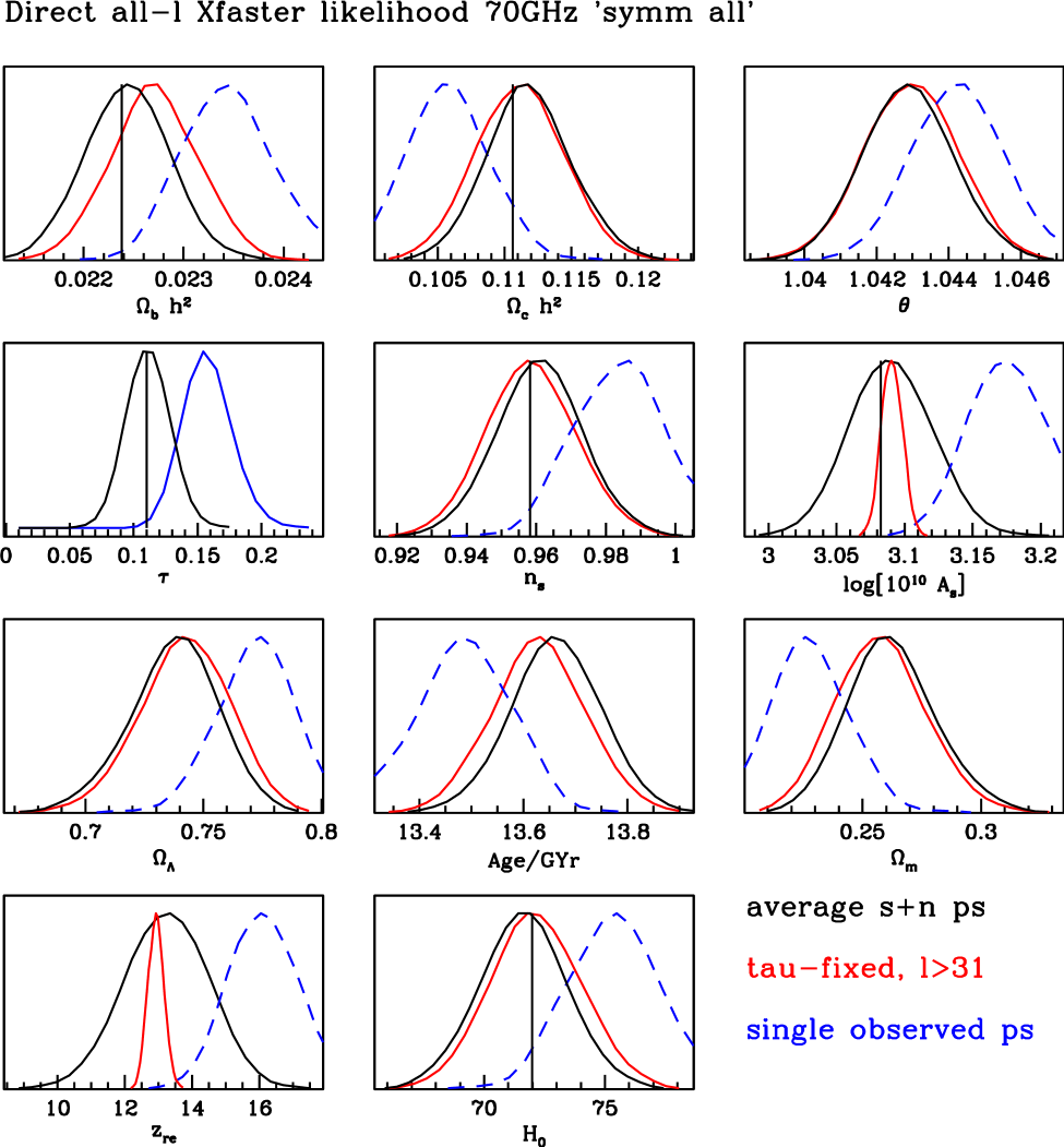
Figure 1, from Rocha et al. (2009), shows one-dimensional marginalised parameter distributions from Xfaster, for three cases: 1) the observed map; the ensemble average of Monte Carlo simulations; and the observed map, but holding fixed at its input value and using the Xfaster likelihood only for . The input parameters are recovered quite well from the ensemble average. The red lines show that if is fixed, high- codes such as XFaster can ignore the low multipoles that they are not designed to calculate, and still recover the other input parameters quite well.
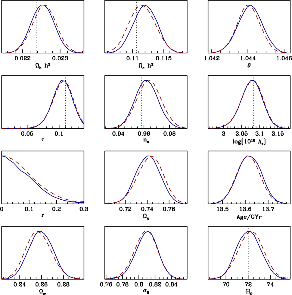
Figure 2 shows parameter distributions from the Offset Lognormal Bandpower likelihood for a Fisher-weighted () window function, for both the observed map and for the ensemble average of Monte Carlo simulations. The input parameters are recovered from the ensemble average simulated data, but not from the observed map, particularly . This is a not a surprise. As described in § 3.1, the observed map is fixed by WMAP for . It is therefore affected by low- anomalies arising from any cause, including the details of WMAP processing. The WMAP best-fit parameters, on the other hand, are obtained with heavy marginalization of the low- points by foregrounds, and are therefore little affected by the low- anomalies. Since the Monte Carlo simulations are realizations of the WMAP best-fit model parameters, we expect no systematic bias from the ensemble of simulations, but significant offsets from the parameters derived from the observed map, as confirmed.
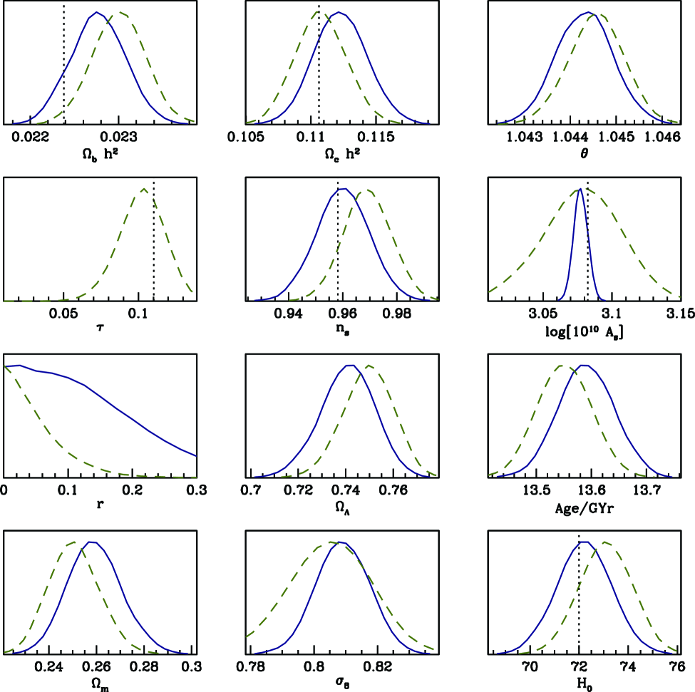
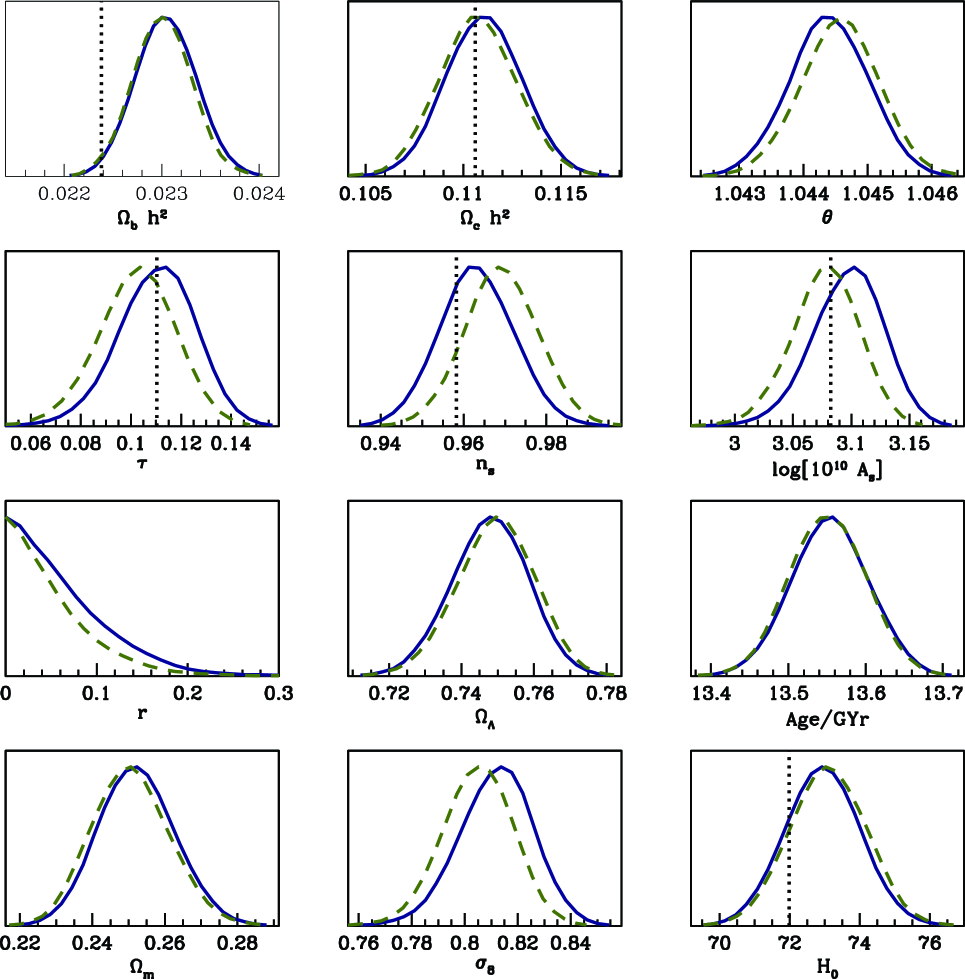
Figure 3 shows the effect of fixing in the case of the Offset Lognormal Bandpower likelihood for a top-hat window function for the observed map. Green dashed lines are computed from all multipoles, with free to vary, while for the blue solid lines use only , with fixed at the input value. As with XFaster in Figure 1, fixing and ignoring low multipoles gives good results with the other parameters.
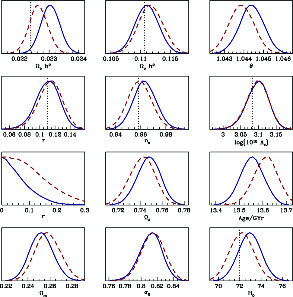
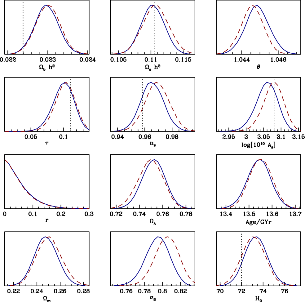
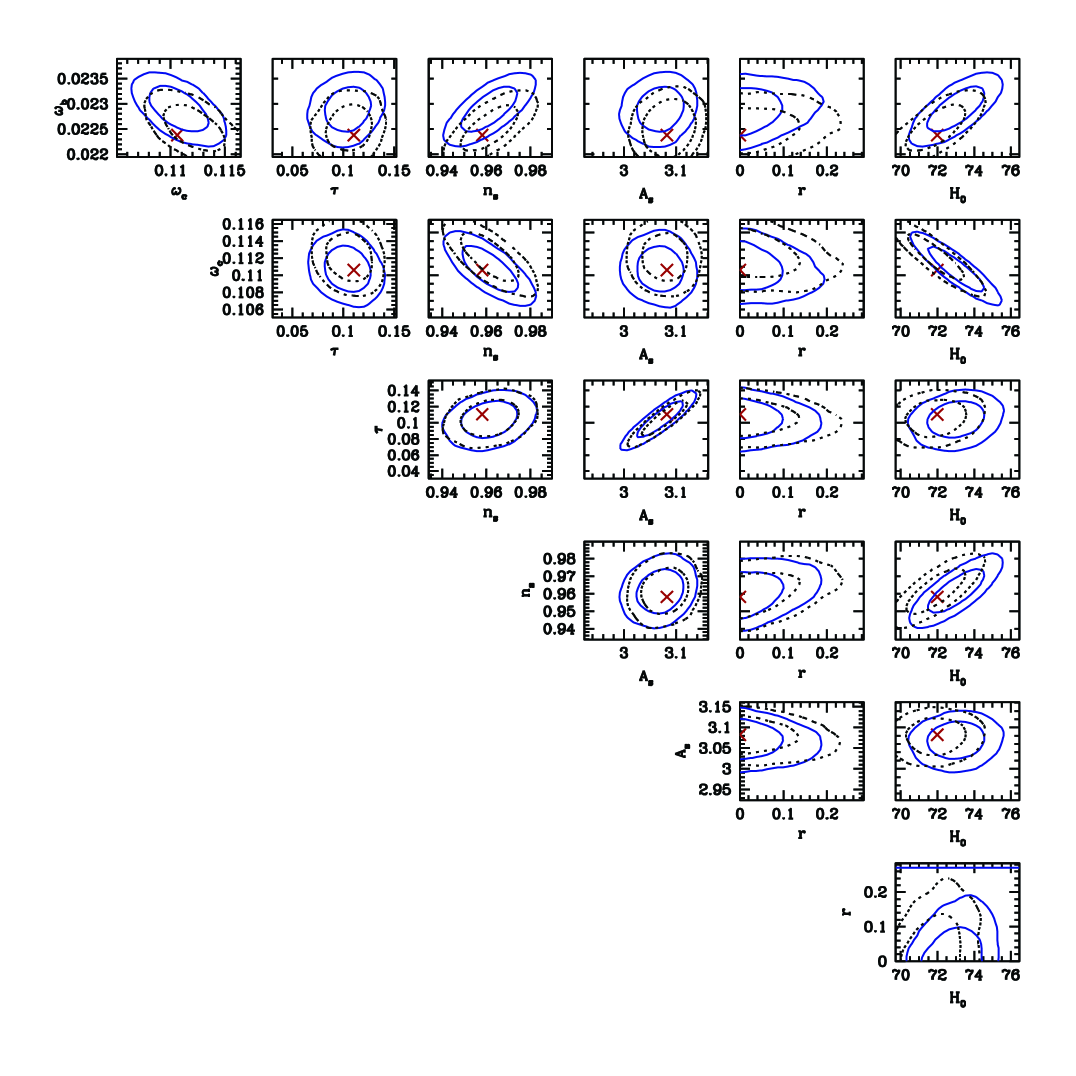
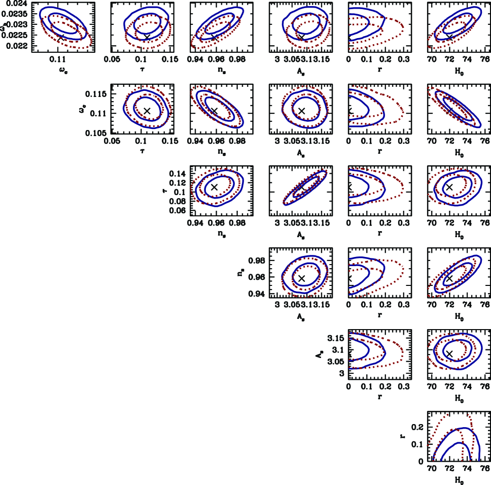
Figures 4 and 5 show parameter distributions from the Offset Lognormal Bandpower likelihood in the symmetric and asymmetric beam cases, for the observed power spectrum and the ensemble average of the Monte Carlo simulations, respectively. Parameters for the two cases are roughly consistent with each other. They can be compared to the equivalent distributions from XFaster likelihood in Figure 21 of Rocha et al. (2009).
Investigating the plot for the average mode, for the case XFaster likelihood we see deviations of the order of for , , and . There is an obvious degeneracy between and . For the observed case these deviations are noticeable mostly in and . Once again these parameters are degenerate.
The overall agreement in the parameter constraints from both symmetric and asymmetric beams is quite impressive. This reflects the adequacy of our procedure when dealing with beam asymmetries, although there is still a slight bias for the asymmetric beam case. This bias is consistent with the small differences in the estimated parameters obtained with the Offset Lognormal Bandpower likelihood, in particular for parameters such as , and . Although the power spectra look consistent, the parameter estimation shows departures of the order of for some of the parameters.
XFaster assumes that the noise is white (uncorrelated), i.e., that the noise covariance matrix is diagonal. Also, the XFaster likelihood is estimated multipole by multipole, unlike the Offset Lognormal Bandpower likelihood. Hence a proper estimation of the transfer function (filter function) requires a large number of Monte Carlo simulations to reduce the correlations between multipoles introduced by, e.g., sky cuts. These simulations include both correlated noise and a sky cut. Hence for the small set of 100 Monte Carlos used here we should expect a larger deviation when XFaster likelihood is employed.
Figures 6, 7, and 8 compare the effect of top-hat and Fisher () window functions on parameters estimated with the Offset Lognormal Bandpower likelihood. Fisher-weighted window functions account for the band power spectrum correlations. It is clear that most parameters improve with windows, while uncertainties for all but are unaffected. The 95% upper limit on is higher by 15% for windows.
Rocha et al. (2009) give a table of parameter constraints obtained with XFaster likelihood for the symmetric beam case. Table 1 is the same for the Offset Lognormal Bandpower likelihood and the XFaster likelihood for the ensemble average power spectrum of the Monte Carlo simulations. Our aim is solely to check how the parameter uncertainties for Planck from both likelihoods compare to those of WMAP (Dunkley et al. 2009) and to our Fisher predictions. The uncertainties are 2–3 times better than those for WMAP except for estimated with the Offset Lognormal Bandpower likelihood, for which the uncertainty on is 0.015 compared to 0.007 for XFaster, 0.017 for WMAP, and 0.004 for our Fisher predictions (Rocha et al. (2004), Table 1).
|
4 Conclusions
Parameters estimated with the XFaster and Offset Lognormal Bandpower likelihoods agree well. As the XFaster likelihood is estimated for individual multipoles, a large number of Monte Carlo simulations is required for accurate estimates of low- correlations. If only a small number of Monte Carlo simulations (such as the 100 used in this study), binning of the band power spectrum estimated with XFaster used along with the Offset Lognormal Bandpower likelihood helps to partially correct these correlations. For a large number of Monte Carlo simulations this is unnecessary. There XFaster likelihood, however, has at least three advantages. First, the Offset Lognormal likelihood does not properly take into account the temperature-polarization cross power. This is likely to become evident with a larger number of simulations, or at lower noise levels, such as anticipated with the Planck HFI 143 GHz channel. We are investigating this further; results will be presented in Rocha et al. (2010). Second, the Offset Lognormal Bandpower likelihood requires calculation of a window function. Third, the XFaster likelihood can go straight from maps to parameters (via its raw pseudo-), bypassing the band power spectrum estimation step. These advantages make XFaster a adequate procedure to estimate cosmological parameters from Planck data in the high multipole regime. As a bonus, XFaster performs reasonably well for moderately low multipoles as well. Although hybridization with a likelihood code able to handle fully the challenges of multipoles less than, say, 40, will be necessary for the best estimates parameters, XFaster could be used alone where accuracy can be traded for speed.
5 Acknowledgments
The work reported in this paper was partially done within the CTP Working Group of the Planck Consortia. Planck is a mission of the European Space Agency. GR would like to thank useful discussions with Jeff Jewell. This research used resources of the National Energy Research Scientific Computing Center, which is supported by the Office of Science of the U.S. Department of Energy under Contract No. DE-AC03-76SF00098. This work has made use of the HEALPix package (Gorski et al. 2005), and of the Planck satellite simulation package, LevelS, (Reinecke et al. 2005), which is assembled by the Max Planck Institute for Astrophysics Planck Analysis Centre (MPAC). The Planck Project in the US is supported by the NASA Science Mission Directorate. The research described in this paper was partially carried out at the Jet propulsion Laboratory, California Institute of Technology, under a contract with NASA. Copyright 2009. All rights reserved.
References
- Ashdown et al. (2007a) Ashdown M. A. J., Baccigalupi C., Balbi A., Bartlett J. G., et al., A&A, 467,761, 2007a
- Ashdown et al. (2007b) Ashdown M., et al., A&A, 471,361, 2007b
- Ashdown et al. (2009) Ashdown M. A. J., Baccigalupi C., Balbi A., Bartlett J. G., et al., A&A, 493,753, 2009
- Ashdown (2009b) Ashdown M. A. J., 2009b, in preparation
- Ashdown et al. (2010) Ashdown M. A. J., Baccigalupi C., Balbi A., Bartlett J. G., et al., 2010, in preparation
- Bond, Jaffe, & Knox (2000) Bond J. R., Jaffe A. H., Knox L., 2000, ApJ, 533, 19
- Contaldi et al. (2009) Contaldi C. R., Bond J. R., Crill, Hivon E., et al., 2009, in preparation
- Dunkley et al. (2009) Dunkley J. et al., Astrophys. J. Suppl. 180 (2009) 306
- Fendt & Wandelt ( 2006) Fendt W. A., Wandelt B. D., Astrophys. J. 654 (2006) 2
- Gorski et al. (2005) Górski K. M., Hivon E., Banday A. J., Wandelt B. D., et al., ApJ, 622, 759-771, 2005
- Hamimeche & Lewis (2008) Hamimeche S., Lewis A., 2008, astro-ph/08010554
- Lewis and Bridle (2002) Lewis A. and Bridle S., 2002, Phys. Rev. D 66, 103511
- Planck Blue Book (2005) Planck Collaboration, Planck Blue Book, [arXiv:astro-ph/0604069].
- Poutanen (2005) Poutanen T., de Gasperis G., Hivon E., Kurki-Suonio H., et al., A&A, 449, 1311, 2006
- Reinecke et al. (2005) Reinecke M., Dolag K., Hell R., Bartelmann M. and Ensslin T., 2005
- Rocha et al. (2004) Rocha G., Trotta R., Martins C. J. A. P., Melchiorri A., Avelino P. P., Bean R. and Viana P. T.,2004, MNRAS, 352, 20R
- Rocha et al. (2009) Rocha G., Contaldi C., Bond D., Górski K. M., 2009, submitted to MNRAS
- Rocha et al. (2010) Rocha G., Contaldi C.R., Bond J.R., Górski K.M., 2010, in preparation
- Smith, Challinor, & Rocha (2006) Smith S., Challinor A., Rocha G., 2006, Phys. Rev. D37, 023517
- Tauber et al. (2009) Tauber J., Mandolesi N., Puget J. L., Bersanelli M., et al., Planck Pre-Launch Status: The Planck Mission, 2009, submitted to A&A
- Tegmark & de Oliveira-Costa (2001) Tegmark M., & de Oliveira-Costa A., 2001, Phys.Rev. D64, 063001
- Verde et al. (2003) Verde L., Peiris H. V., Spergel D. N., Nolta M. R., et al., 2003, ApJS, 148, 195