THREE LECTURES: NEMD, SPAM, and SHOCKWAVES

Abstract

We discuss three related subjects well suited to graduate research. The first, Nonequilibrium molecular dynamics or “NEMD”, makes possible the simulation of atomistic systems driven by external fields, subject to dynamic constraints, and thermostated so as to yield stationary nonequilibrium states. The second subject, Smooth Particle Applied Mechanics or “SPAM”, provides a particle method, resembling molecular dynamics, but designed to solve continuum problems. The numerical work is simplified because the SPAM particles obey ordinary, rather than partial, differential equations. The interpolation method used with SPAM is a powerful interpretive tool converting point particle variables to twice-differentiable field variables. This interpolation method is vital to the study and understanding of the third research topic we discuss, strong shockwaves in dense fluids. Such shockwaves exhibit stationary far-from-equilibrium states obtained with purely reversible Hamiltonian mechanics. The SPAM interpolation method, applied to this molecular dynamics problem, clearly demonstrates both the tensor character of kinetic temperature and the time-delayed response of stress and heat flux to the strain rate and temperature gradients. The dynamic Lyapunov instability of the shockwave problem can be analyzed in a variety of ways, both with and without symmetry in time. These three subjects suggest many topics suitable for graduate research in nonlinear nonequilibrium problems.

I Thermodynamics, Statistical Mechanics, and NEMD

I.1 Introduction and Goals

Most interesting systems are nonequilibrium ones, with gradients in velocity, pressure, and temperature causing flows of mass, momentum, and energy. Systems with large gradients, so that nonlinear transport is involved, are the most challenging. The fundamental method for simulating such systems at the particle level is nonequilibrium molecular dynamics (NEMD).b1 ; b2 ; b3 Nonequilibrium molecular dynamics couples together Newtonian, Hamiltonian, and Nosé-Hoover mechanics with thermodynamics and continuum mechanics, with the help of Gibbs’ statistical mechanics, and Maxwell and Boltzmann’s kinetic theory. Impulsive hard-sphere collisions or continuous interactions can both be treated.

NEMD necessarily includes microscopic representations of the macroscopic thermodynamic energy $E$, pressure and temperature tensors $P$ and $T$, and heat-flux vector $Q$. The underlying microscopic-to-macroscopic connection is made by applying Boltzmann and Gibbs’ statistical phase-space theories, generalized to include Green and Kubo’s approach to the evaluation of transport coefficients, together with Nosé’s approach to introducing thermostats, ergostats, and barostats into particle motion equations.

These temperature, energy, and pressure controls make it possible to simulate the behavior of a wide variety of nonequilibrium flows with generalized mechanics. The nonequilibrium phase-space distributions which result are typically multifractal, as is illustrated here with a few examples taken from our website, [ http://williamhoover.info ]. These ideas are summarized in more detail in the books “Molecular Dynamics”, “Computational Statistical Mechanics” and “Time Reversibility, Computer Simulation, and Chaos”. The one-particle “Galton Board” (with impulsive forces) and the “thermostated nonequilibrium oscillator” problem (with continuous forces) are simple enough for thorough phase-space analyses. Macroscopic problems, like the steady shockwave and Rayleigh-Bénard flow, can be analyzed locally in phase space by computing local growth rates and nonlocal Lyapunov exponents.

The main goal of all this computational work is “understanding”, developing simplifying pictures of manybody systems. The manybody systems themselves are primarily computational entities, solutions of ordinary or partial differential equations for model systems. Quantum mechanics and manybody forces are typically omitted, mostly for lack of compelling and realistic computer algorithms. There is an enduring gap between microscopic simulations and realworld engineering. The uncertainties in methods for predicting catastrophic failures will continue to surprise us, no matter the complexity of the computer models we use to “understand” systems of interest.

Number-dependence in atomistic simulations is typically small: $1/N$ for the thermodynamic properties of periodic $N$-body systems, perhaps $1/\sqrt{N}$ or even $1/\ln N$ in problems better treated with continuum mechanics. So far we have come to understand the equilibrium equation of state, the linear transport coefficients, the Lyapunov instability of manybody trajectories, and the irreversibility underlying the Second Law. Improved understanding of relatively-simple hydrodynamic flows, like the Rayleigh-Bénard flow treated here, will follow from the special computational techniques developed to connect different length scales. Smooth Particle Applied Mechanics, “SPAM”,b4 ; b5 ; b6 has proved itself as not only a useful simulation technique for continuum systems, but also as a powerful interpolation tool for all point-particle systems, as is illustrated here for the shockwave problemb7 ; b8 ; b9 .

I.2 Development of Molecular Dynamics at and Away from Equilibrium

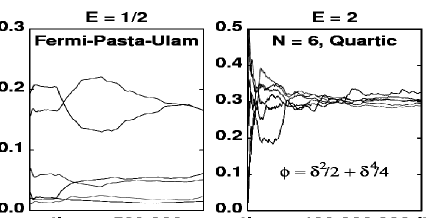
In the early days of expensive vacuum-tube computing the hardware and software were largely controlled by the Federal Government and located at the various weapons and energy laboratories at Argonne, Brookhaven, Livermore, Los Alamos and Oak Ridge. Fermi developed molecular dynamics at the Los Alamos Laboratory in the summers of 1952-1953, discovering many of the interesting nonergodic recurrence features characterizing the low-energy behavior of one-dimensional anharmonic “Fermi-Pasta-Ulam chains”. The Los Alamos Report summarizing his work was prepared a few months after his deathb10 ; b11 ; b12 . At sufficiently low energies the anharmonic chains showed no tendency toward equilibration while (it was discovered much later that) at higher energies they did. Figure 1 shows time-averaged “mode energies” for a six-particle chain with two different initial conditions. In both cases the nearest-neighbor potential generates both linear and cubic forces:

$$\phi(r)=(1/2)(r-1)^{2}+(1/4)(r-1)^{4}\ .$$

Initially we choose the particles equally spaced and give all the energy to Particle 1, $E=p_{1}^{2}/2$. The left side of the Figure corresponds to an initial momentum of 1 while the right side follows a similarly long trajectory (100 million Runge-Kutta timesteps) starting with the initial momentum $p_{1}=2$. Fermi was surprised to find that at moderate energies there was no real tendency toward equilibration despite the anharmonic forces. Thus the averaging techniques of statistical mechanics can’t usefully be applied to such oversimplified systems.

Figure 1: The time averages of the six harmonic mode energies (calculated just as was done by Benettinb12 ) are shown as functions of time for two different initial conditions, with total energies of 0.5 and 2.0. The six-particle chain of unit mass particles with least-energy coordinates of $\pm 0.5,\pm 1.5,\ {\rm and}\ \pm 2.5$ is bounded by two additional fixed particles at $\pm 3.5$.

Fermi also carried out some groundbreaking two-dimensional work. He solved Newton’s equations of motion,

$$\{\ m\ddot{r}=F(r)\ \}\ ,$$

and didn’t bother to describe the integration algorithm. A likely choice would be the time-reversible centered second-difference “Leapfrog” algorithm,

$$\{\ r_{t+dt}=2r_{t}-r_{t-dt}+(F/m)_{t}(dt)^{2}\ \}\ ,$$

where the timestep $dt$ is a few percent of a typical vibrational period. The dominant error in this method is a “phase error”, with the orbit completing prematurely. A harmonic oscillator with unit mass and force constant has a vibrational period of $2\pi$. The second-difference Leapfrog algorithm’s period is 6, rather than 6.2832, for a relatively large timestep, $dt=1$. A typical set of six (repeating) coordinate values for this timestep choice is:

$$\{\ +2,+1,-1,-2,-1,+1,\ \dots\ \}$$

The Leapfrog algorithm diverges, with a period of $2\sqrt{2}$, as $dt$ approaches $\sqrt{2}$.

Vineyard used the Leapfrog algorithm at the Brookhaven Laboratory, including irreversible viscous quiet-boundary forces designed to minimize the effect of surface reflections on his simulations of radiation damageb13 . Alder and Wainwright, at the Livermore Laboratory, studied hard disks and spheres in parallel with Wood and Jacobsen’s Monte Carlo work at the Los Alamos laboratory, finding a melting/freezing transition for spheresb14 ; b15 . The disks and spheres required different techniques, with impulsive instantaneous momentum changes at discrete collision times. All these early simulations gave rise to a new discipline, “molecular dynamics”, which could be used to solve a wide variety of dynamical problems for gases, liquids, and solids, either at, or away from, equilibrium. By the late 1960s the results of computer simulation supported a successful semiquantitative approach to the equilibrium thermodynamics of simple fluidsb16 .

In the 1970s Ashurstb17 (United States), Dreminb18 (Union of Soviet Socialist Republics), Verletb19 (France), and Woodcockb20 (United Kingdom), were among those adapting molecular dynamics to the solution of nonequilibrium problems. Shockwaves, the subject of our third lecture, were among the first phenomena treated in the effort to understand the challenging problems of far-from-equilibrium many-body systems.

I.3 Temperature Control à la Nosé

Shuichi Nosé made a major advance in 1984b21 ; b22 , developing a dynamics, “Nosé-Hoover dynamics”, which provides sample isothermal configurations from Gibbs’ and Boltzmann’s canonical distribution,

$$f(q,p)\propto e^{-{\cal H}(q,p)/kT}\ ;\ {\cal H}(q,p)=\Phi(q)+K(p)\ .$$

The motion equations contain one or more friction coefficients $\{\zeta\}$ which influence the motion, forcing the longtime average of one or more of the $p_{i}^{2}$ to be $mkT_{i}$:

$$\{\ m\ddot{r}_{i}=F_{i}-\zeta_{i}p_{i}\ ;\ \dot{\zeta}_{i}=[(p_{i}^{2}/mkT_{i})-1]/\tau_{i}^{2}\ \}\ .$$

The thermostat variable $\zeta$ can introduce or extract heat. The adjustable parameter $\tau$ is the characteristic time governing the response of the thermostat variable $\zeta$. A useful special case that follows from Nosé’s work in the limit $\tau\rightarrow 0$ is “Gaussian” isokinetic dynamics, a dynamics with fixed, rather than fluctuating, kinetic energy $K(p)=K_{0}$,

In 1996 Dettmann showed that the Nosé-Hoover equations of motion follow generally from a special Hamiltonian, without the need for the time scaling Nosé used in his original work:

$${\cal H}_{\rm Dettmann}=s[\Phi(q)+K(p/s)+\#kT\ln s+\#kT(p_{s}\tau)^{2}/2]\equiv 0\ .$$

Here the friction coefficient is $\zeta\equiv\#kT\tau^{2}p_{s}$, where $p_{s}$ is the Hamiltonian momentum conjugate to $s$. The trick of setting the Hamiltonian equal to a special value, 0, is essential to Dettmann’s derivationb23 .

Consider the simplest interesting case, a harmonic oscillator with unit mass, force constant, temperature, and relaxation time:

$${\cal H}=s[q^{2}+(p/s)^{2}+\ln s^{2}+p_{s}^{2}]/2=0\rightarrow$$

$$\dot{q}=(p/s)\ ;\ \dot{p}=-sq\ ;\ \dot{s}=sp_{s}\ ;\ \dot{p}_{s}=-[0]+(p/s)^{2}-1\ \rightarrow$$

$$\ddot{q}=(1/s)\dot{p}-(p/s)(\dot{s}/s)=-q-\zeta\dot{q}\ ;\ \dot{p}_{s}\equiv\dot{\zeta}=\dot{q}^{2}-1\ .$$

The time average of the $\dot{\zeta}$ equation shows that the longtime average of $\dot{q}^{2}$ is unity. In particular applications $\tau$ should be chosen to maximize the efficiency of the simulation by minimizing the necessary computer time.

Runge-Kutta integration is a particularly convenient method for solving such sets of coupled first-order differential equations. The fourth-order method is the most useful. The time derivative is an average from four evaluations, $\{\ \dot{y}_{0},\dot{y}_{1},\dot{y}_{2},\dot{y}_{3}\ \}$, of the righthand sides of all the differential equations, here collected in the form of a single differential equation for the vector $y$:

$$y_{1}=y_{0}+(dt/2)\dot{y}_{0}\ ;\ y_{2}=y_{0}+(dt/2)\dot{y}_{1}\ ;\ y_{3}=y_{0}+dt\dot{y}_{2}\ ;$$

$$y_{dt}=y_{0}+(dt/6)[\dot{y}_{0}+2\dot{y}_{1}+2\dot{y}_{2}+\dot{y}_{3}]\ .$$

The Runge-Kutta energy decays with time as $dt^{5}$ at a fixed time for a chosen timestep $dt$. Here the vector $y$ is $(q,p)$ so that

$$\dot{y}\equiv(\dot{q},\dot{p})\equiv(+p,-q)\ .$$

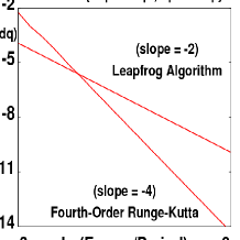
For small $dt$ the Runge-Kutta trajectory for a harmonic oscillator with the exact trajectory $q=\cos(t)$ has an error $\delta q=+dt^{4}t\sin(t)/120$. The corresponding Leapfrog error is $\delta q=-dt^{2}t\sin(t)/24$. The two methods should give equally good solutions (where the two curves in the Figure cross) when

$$dt_{\rm LF}\simeq dt_{\rm RK}/4=\sqrt{5/256}\simeq 0.14\ ,$$

corresponding to about 45 force evaluations per oscillator periodb24 .

For a 14-digit-accurate trajectory calculation, with $dt_{RK}=0.001$ and $dt_{LF}=0.00025$, the Runge-Kutta error would be smaller than the Leapfrog error by seven orders of magnitude. At the cost of additional programming complexity choosing one of the fourth-order Gear integrators can reduce the integration error by an additional factor of $\simeq 60$b25 .

Figure 2: Comparison of the maximum error (which occurs near a time of $3\pi/2$), in a harmonic oscillator coordinate for the Leapfrog and Fourth-Order-Runge-Kutta integrators. The abscissa shows the logarithm of the number of force evaluations (which varies from about 20 to about 400) used during a full vibrational period, $2\pi$. The oscillator equations of motion are $\dot{q}=p\ ;\ \ddot{q}=\dot{p}=-q$.

I.4 Connecting Microscopic Dynamics to Macroscopic Physics

To connect the microscopic dynamics to macroscopic thermodynamics and continuum mechanics is quite easy for a homogeneous system confined to the volume $V$. A numerical solution of the equations of motion for the coordinates and momenta, $\{\ q,p\ \}$, makes it possible to compute the energy $E$, the temperature tensor $T$, the pressure tensor $P$, and the heat-flux vector $Q$:

$$E=\Phi(q)+K(p)=\sum_{i<j}\phi_{ij}+\sum_{i}p_{i}^{2}/(2m)\ ;\$$

$$T_{xx}=\langle p_{x}^{2}/mk\rangle=\sum_{i}(p_{x}^{2}/mk)_{i}/N\ ;\ T_{yy}=\langle p_{y}^{2}/mk\rangle\ ;$$

$$PV=\sum_{i<j}F_{ij}r_{ij}+\sum_{i}(pp/mk)_{i}\ ;\$$

$$QV=\sum_{i<j}F_{ij}\cdot p_{ij}r_{ij}+\sum_{i}(ep/mk)_{i}\ .\$$

These expressions can be derived directly from the dynamics, by computing the mean momentum and energy fluxes (flows per unit area and time) in the volume $V$. Alternatively they can be derived by multiplying the Newtonian equations of motion by $(p/m)$ (giving the “Virial Theorem”) or by $e$ (giving the “Heat Theorem”) and time averagingb1 . We will see that local versions of these definitions lead to practical implementations of numerical hydrodynamics at atomistic length and time scales.

The thermomechanical bases of these relations are statistical mechanics and kinetic theory. Hamilton’s mechanics yields Liouville’s theorem for the time derivative of the many-body phase-space probability density following the motion:

$$\dot{f}/f=d\ln f/dt=0\ {\rm[Hamiltonian\ Mechanics]}\ ;$$

Nosé-Hoover mechanics opens up the possibility for $f$ to change:

$$\dot{f}/f=d\ln f/dt=\zeta=-\dot{E}/kT=\dot{S}_{\rm ext}/k\ {\rm[Nos\acute{e}-Hoover\ Mechanics]}\ .$$

The primary distinction between nonequilibrium and equilibrium systems lies in the friction coefficients $\{\ \zeta\ \}$. At equilibrium (ordinary Newtonian or Hamiltonian dynamics) the average friction vanishes while in nonequilibrium steady states $\langle\sum k\zeta\rangle=\dot{S}_{\rm ext}>0$ it is equal to the time-averaged entropy production rate.

In any stationary nonequilibrium state the sum of the friction coefficients is necessarily positive – a negative sum would correspond to phase-space instability incompatible with a steady state. An important consequence of the positive friction is that the probability density for these states diverges as time goes on, indicating the collapse of the probability density onto a fractal strange attractor. Fractals differ from Gibbs’ smooth distributions in that the density is singular, and varies as a fractional power of the coordinates and momenta in phase spaceb2 ; b26 ; b27 ; b28 ; b29 .

I.5 Fractal Phase-Space Distributions

The harmonic oscillator problem is not ergodic with Nosé-Hoover dynamics. One way to make it so is to fix the fourth moment of the velocity distribution as well as the second. This improvement also makes it possible to study interesting nonequilibrium oscillator-based problems, such as the conduction of energy from hot to cold through the oscillator motion. Figure 3 shows the time development of (the two-dimensional projection of) such a problem. The isothermal oscillator, along with two friction coefficients, $\{\zeta,\xi\}$, fixing the second and fourth moments, $\langle(p^{2},p^{4})\rangle$ has a Gaussian distribution in its four-dimensional phase space. A special nonisothermal case, with a coordinate-dependent temperature leading to heat flow, generates a 2.56-dimensional fractal in the four-dimensional $\{q,p,\zeta,\xi\}$ phase space. The dynamics governing this continuous nonequilibrium motion is as follows:

$$\dot{q}=p\ ;\ \dot{p}=-q-\zeta p-\xi p^{3}\ ;$$

$$\dot{\zeta}=[p^{2}-T]\ ;\ \dot{\xi}=[p^{4}-3p^{2}T]\ ;\ T=T(q)=1+\tanh(q)\ .$$

Here time averages of the control-variable equations show that the second and fourth moments satisfy the usual thermometric definitions:

$$\langle p^{2}\rangle=\langle T\rangle\ ;\ \langle p^{4}\rangle=3\langle p^{2}T\rangle\ .$$

The phase-space distribution for this oscillator has an interesting fractal natureb26 ; b27 . Figure 3 shows how the continuous trajectory comes to give a fractal distribution, as is typical of thermostated nonequilibrium problems. Besides the æsthetic interest that this model provides, it illustrates the possibilities for controlling moments of the velocity distribution beyond the first and second, as well as the possibility of introducing a coordinate-dependent temperature directly into the motion equations.

Figure 3: This $(\zeta,\xi)$ projection of the doubly-thermostated oscillator fractal is shown at five successive stages of temporal resolution. The time intervals between successive points range from 0.001, the Runge-Kutta timestep, to 10.0, showing how a continuous trajectory can lead to a fractal object.

Figure 4: Sierpinski Sponge, constructed by removing 7 of the 27 equal cubes contained in the unit cube, leaving 20 smaller cubes, and then iterating this process ad infinitum leaving a 2.727-dimensional fractal of zero volume.

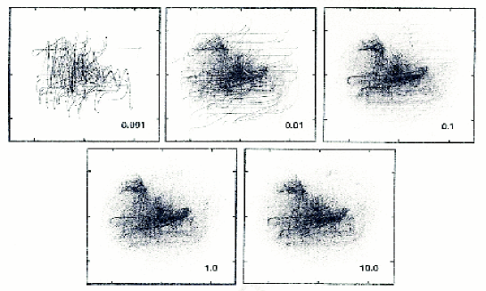
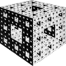
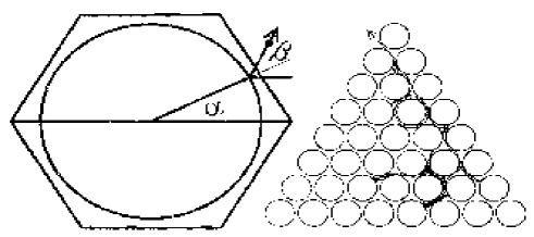
Figure 4 shows a more typical textbook fractal, the Sierpinski sponge, in which the probability density is concentrated on a set of dimension 2.727. In almost all of the largest cube the density vanishes. Unlike the multifractal of Figure 3, the Sierpinski sponge is homogeneous, so that an $n$-fold enlarged view of a small part of the sponge, with an overall volume $1/27^{n}$ of the total, looks precisely like the entire object.

I.6 The Galton Board

The situation with impulsive forces is quite different. Whenever impulsive collisions occur the phase-space trajectory makes a jump in momentum space, from one phase point to another. Consider the simplest interesting case: a single point mass, passing through a triangular lattice of hard scatterersb2 ; b30 ; b31 . That model generates exactly the same ergodic dynamics as does a periodic two-hard-disk system with no center-of-mass motion:

$$r_{1}+r_{2}=0\ ;\ v_{1}+v_{2}=0\ .$$

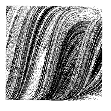
By adding a constant field and an isokinetic thermostat to the field-dependent motion, the trajectory tends smoothly toward the field direction until a collisional jump occurs. Over long times (Figure 5 is based on 200,000 collisions) an extremely interesting nonequilibrium stationary state results, with a fractal phase-space distribution. The example shown in the Figure has an information dimension of 1.832. As a consequence, the coarse-grained entropy, $-k\langle f\ln f\rangle$, when evaluated with phase-space cells of size $\delta$, diverges as $\delta^{-0.168}$, approaching minus infinity as a limiting case.

The probability densities for nonequilibrium steady states, such as the Galton Board, shown in Figure 5, are qualitatively different to the sponge, where the probability density is equally singular wherever it is nonzero. The Galton Board’s nonequilibrium probability density is nonzero for any configuration consistent with the initial conditions on the dynamics. Further, the (multi)fractal dimension of these inhomogeneous distributions varies throughout the phase space.

The concentrated nature of the nonequilibrium probability density shows first of all that nonequilibrium states are very rare in phase space. Finding one by accident has probability zero. The time reversibility of the equations of motion additionally shows that the probability density going forward in time contracts (onto a strange attractor), and so is necessarily stable relative to a hypothetical reversed trajectory going backward in time, which would expand in an unstable way. This symmetry breaking is a microscopic equivalent of the Second Law of Thermodynamics, a topic to which we’ll return. It is evidently closely related to the many “fluctuation theorems”b32 ; b33 which seek to give the relative probabilities of forward and backward nonequilibrium trajectories as calculated from Liouville’s Theorem.

Figure 5: A series of 200,000 Galton Board collisions are plotted as separate points, with ordinate $-1<\sin(\beta)<1$ and abscissa $0<\alpha<\pi$, where $\alpha$ is measured relative to the field direction, as shown in Figure 6.

Figure 6: The Galton Board geometry is shown, defining the angles $\alpha$ and $\beta$ identifying each collision. The unit cell shown here, extended periodically, is sufficient to describe the problem of a moving particle in an infinite lattice of scatterers.

I.7 Determination of Transport Coefficients via NEMD

With measurement comes the possibility of control. Feedback forces, based on the results of measurement, can be used to increase or decrease a “control variable” (such as the friction coefficient $\zeta$ which controls the kinetic temperature through a “thermostating” force). Equations of motion controlling the energy, or the temperature, or the pressure, or the heat flux, can all be developed in such a way that they are exactly consistent with Green and Kubo’s perturbation-theory of transportb2 ; b3 . That theory is a first-order perturbation theory of Gibbs’ statistical mechanics. It expresses linear-response transport coefficients in terms of the decay of equilibrium correlation functions. For instance, the shear viscosity $\eta$ can be computed from the decay of the stress autocorrelation function:

$$\eta=(V/kT)\int_{0}^{\infty}\langle P_{xy}(0)P_{xy}(t)\rangle_{\rm eq}dt\ ,$$

and the heat conductivity $\kappa$ can be computed from the decay of the heat flux autocorrelation function:

$$\kappa=(V/kT^{2})\int_{0}^{\infty}\langle Q_{x}(0)Q_{x}(t)\rangle_{\rm eq}dt\ .$$

Nosé’s ideas have made it possible to simulate and interpret a host of controlled nonequilibrium situations. A Google search for “Nosé-Hoover” in midJuly of 2010 produced over eight million separate hits.

Figure 7: A Four Chamber viscous flow. Solid blocks (filled circles), move antisymmetrically to the left and right, so as to shear the two chambers containing Newtonian fluid (open circles). This geometry makes it possible to characterize the nonlinear differences among the diagonal components of the pressure and temperature tensors.

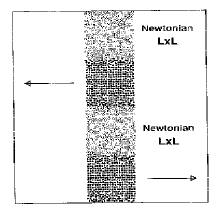
Figure 7 shows a relatively-simple way to obtain transport coefficients using nonequilibrium molecular dynamics. Ashurstb17 , in his thesis work at the University of California, “Dense Fluid Shear Viscosity and Thermal Conductivity via Molecular Dynamics”, introduced two “fluid walls”, with different specified velocities and/or temperatures, in order to simulate Newtonian viscosity and Fourier heat flow. Figure 7, a fully periodic variation of Ashurst’s idea, shows two “reservoir” regions, actually “solid walls”, separating two Newtonian regions. In both the Newtonian regions momentum and energy fluxes react to the different velocities and temperatures imposed in the “wall” reservoirs. This four-chamber technique produces two separate nonequilibrium profilesb34 ; b35 ; b36 .

In the Newtonian chambers, where no thermostat forces are exerted, the velocity or temperature gradients are nearly constant, so that accurate values of the viscosity and heat conductivity can be determined by measuring the (necessarily constant) shear stress or the heat flux:

$$\eta=-P_{xy}/[(dv_{y}/dx)+(dv_{x}/dy)]\ ;\ \kappa=-Q_{x}/(dT/dx)\ .$$

I.8 Nonlinear Transport

This same “solid-wall” or “four-chamber” method has been used to study a more complicated aspect of nonequilibrium systems, the nonlinear contributions to the fluxes. Because the underlying phase-space distributions are necessarily fractal it is to be expected that there is no analytic expansion of the transport properties analogous to the virial (powers of the density) expansion of the equilibrium pressure. Periodic shear flows, with the mean $x$ velocity increasing linearly with $y$,

$$\{\ \dot{x}=(p_{x}/m)+\dot{\epsilon}y\ ;\ \dot{y}=(p_{y}/m)\ \}\ ;$$

can be generated with any one member of the family of motion equations:

$$\{\ \dot{p}_{x}=F_{x}-\dot{\epsilon}\alpha_{x}p_{y}-\zeta p_{x}\ ;\ \dot{p}_{y}=F_{y}-\dot{\epsilon}\alpha_{y}p_{x}-\zeta p_{y}\ \}\ ,$$

so long as the sum $\alpha_{x}+\alpha_{y}$ is unity and $\zeta$ is chosen to control the overall energy or temperature. Careful comparisons of the two limiting approaches,

$$\alpha_{x}=0\ ;\ \alpha_{y}=1\ {\rm[Doll^{\prime}s]}\ ;$$

$$\alpha_{x}=1\ ;\ \alpha_{y}=0\ {\rm[s^{\prime}lloD]}\ ,$$

with corresponding boundary-driven four-chamber flows show that though both of the algorithms satisfy the nonequilibrium energy requirement:

$$\dot{E}\equiv-\dot{\epsilon}P_{xy}V\ ,$$

exactly, neither of them provides the correct “normal stress” difference, $P_{xx}-P_{yy}$.

This same problem highlights another interesting parallel feature of nonequilibrium systems, the tensor nature of temperatureb7 ; b8 ; b9 ; b37 ; b38 ; b39 ; b40 . In a boundary-driven shearflow with the repulsive pair potential,

$$\phi(r<1)=100(1-r^{2})^{4}\ ,$$

the temperature tensors in the Newtonian regions show the orderings

$$\langle p^{2}_{x}\rangle>\langle p^{2}_{z}\rangle>\langle p^{2}_{y}\rangle\ \longleftrightarrow\ T_{xx}>T_{zz}>T_{yy}\ {\rm[Boundary\ Driven}]\ .$$

The homogeneous periodic shear flows generated with the Doll’s and s’lloD algorithms show instead two other orderings:

$$T_{xx}>T_{yy}>T_{zz}\ {\rm[s^{\prime}lloD]}\ \ {\rm and}\ \ T_{yy}>T_{xx}>T_{zz}\ {\rm[Doll^{\prime}s]}\ ,$$

so that neither the Doll’s nor the s’lloD algorithm correctly accounts for the nonlinear properties of stationary shear flowsb35 . Nonequilibrium molecular dynamics provides an extremely versatile tool for determining nonlinear as will as linear transport. We will come back to tensor temperature in the third lecture, on shockwaves. Nonlinear transport problems can require the definition of local hydrodynamic variables whenever the system is inhomogeneous, as it is in boundary-driven shear and heat flows.

Thermostats, ergostats, barostats, and many other kinds of constraints and controls simplify the treatment of complex failure problems with molecular dynamics. Using the Doll’s and s’lloD ideas it is quite feasible to study the stationary nonequilibrium flow of solids, “plastic flow”, in order to interpret nonsteady failure problems like fracture and indentation. Nonequilibrium molecular dynamics makes it possible to remove the irreversible heat generated by strongly nonequilibrium processes such as the machining of metals. The basic idea of control can be implemented from the standpoint of Gauss’ Principle, which states that the smallest possible constraint force should be used to accomplish controlb41 . Near equilibrium a more reliable basis is Green and Kubo’s linear-response theory. This can be used to formulate controls consistent with exact statistical mechanics in the linear regime, just as was done in deriving the Doll’s and s’lloD approaches to simulating shear flow.

Figure 8: Rayleigh-Bénard problem, simulated with 5000 particles. The fluid-wall image particles which enforce the thermal and velocity boundary conditions are shown as circles above and below the main flow.

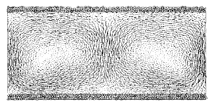
A slightly more complex problem is illustrated in Figure 8. A nonequilibrium system with fixed mass is contained within two thermal “fluid wall” boundaries, hot on the bottom and cold on the top, with a gravitational field acting downward. If the gradients are small the fluid is stationary, and conducts heat according to Fourier’s Law. When the Rayleigh Number,

$$R=gL^{4}(d\ln T/dy)/(\nu\kappa)\ ;\ \nu\equiv\eta/\rho\ ,$$

exceeds a critical value (which can be approximated by carrying out a linear stability analysis of the hydrodynamic equations) two rolls, one clockwise and the other counterclockwise provide another, faster, mode of heat transfer. At higher values of $R$ the rolls oscillate vertically; at higher values still the rolls are replaced by chaotic heat plumes, which move horizontally. With several thousand particles molecular dynamics provides solutions in good agreement with the predictions of the Navier-Stokes-Fourier equations.

This problemb42 ; b43 ; b44 is specially interesting in that several topologically different solutions can exist for exactly the same applied boundary conditions. Carol will talk more about this problem in her exposition of Smooth Particle Applied Mechanics, “SPAM”. SPAM provides a useful numerical technique for interpolating the particle properties of nonequilibrium molecular dynamics onto convenient spatial grids.

II Particle-Based Continuum Mechanics & SPAM

II.1 Introduction and Goals

Smooth Particle Applied Mechanics, “SPAM”, was invented at Cambridge, somewhat independently, by Lucy and by Monaghan in 1977b4 ; b5 ; b6 . The particles both men considered were astrophysical in size as their method was designed to treat clusters of stars. SPAM can be used on smaller scales too. SPAM provides a simple and versatile particle method for solving the continuum equations numerically with a twice-differentiable interpolation method for the various space-and-time-dependent field variables (density, velocity, energy, …) . SPAM looks very much like “Dissipative Particle Dynamics”b45 , though, unlike DPD, it is typically fully deterministic, with no stochastic ingredients. Three pedagogical problems are discussed here using SPAM: the free expansion of a compressed fluid; the collapse of a water column under the influence of gravity; and thermally driven convection, the Rayleigh-Bénard problem. Research areas well-suited to graduate research (tensile instability, angular momentum conservation, phase separation, and surface tension) are also described.

SPAM provides an extremely simple particle-based solution method for solving the conservation equations of continuum mechanics. For a system without external fields the basic partial differential equations we aim to solve are:

$$\dot{\rho}=-\rho\nabla\cdot v\ ;$$

$$\rho\dot{v}=-\nabla\cdot P\ ;$$

$$\rho\dot{e}=-\nabla v:P-\nabla\cdot Q\ .$$

SPAM solves the equations by providing a particle interpretation for each of the continuum variables occuring in these conservation laws. The main difficulty in applying the method involves the choice and implementation of boundary conditions, which vary from problem to problem.

II.2 SPAM Algorithms and the Continuity Equation

The fluid dynamics notation here, $\{\rho,v,e,P,Q\}$, with each of these variables dependent on location $r$ and time $t$, is standard but the SPAM particle interpretation of them is novel. The density $\rho$ and momentum density $(\rho v)$ at any location $r$ are local sums of nearby individual particle contributions,

$$\rho(r)\equiv\sum_{j}m_{j}w(r-r_{j})\ ;\ \rho(r_{i})=\sum_{j}m_{j}w(r_{i}-r_{j})\ ;\ \rho(r)v(r)\equiv\sum_{j}m_{j}v_{j}w(r-r_{j})\ ,$$

where particles have an extent $h$, the “range” of the weight function $w$, so that only those particles within $h$ of the location $r$ contribute to the averages there.

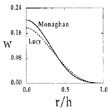
In the second expression (for the density at the particle location $r_{i}$) the “self” term ($r_{i}=r_{j}$) is included so that the two definitions coincide at the particle locations. The weight function $w$, which describes the spatial distribution of particle mass, or region of influence for particle $j$, is normalized, has a smooth maximum at the origin, and a finite range $h$, at which both $w^{\prime}$ and $w^{\prime\prime}$ vanish. The simplest polynomial filling all these needs is Lucy’sb4 ; b5 , here normalized for two-dimensional calculations:

$$w_{2D}(r<h)=(5/\pi h^{2})[1-6x^{2}+8x^{3}-3x^{4}]\ ;\ x\equiv r/h\ .$$

Monaghan’s weight function, shown for comparison in the Figure, uses two different polynomials in the region where $w$ is nonzero. The range $h$ of $w(r<h)$ is typically a scalar, chosen so that a few dozen smooth particles contribute to the various field-point averages at a point. As shown in Figure 9 Lucy’s function looks much like a Gaussian, but vanishes very smoothly as $r\rightarrow h$. By systematically introducing the weight function into expressions for the instantaneous spatial averages of the density, velocity, energy, pressure, and heat flux, the continuum equations at the particle locations become ordinary differential equations much like those of molecular dynamics. The method has the desirable characteristic that the continuum variables have continuous first and second spatial derivatives.

Figure 9: Lucy’s and Monaghan’s weight functions. Both functions are normalized for two space dimensions and $h=3$. The weight function $w(r<h)$ describes the spatial influence of particles to properties in their neighborhood, as explained in the text.

The continuity equation (conservation of mass) is satisfied automatically. At a fixed point $r$ in space, the time derivative of the density depends upon the velocities of all those particles within the range $h$ of $r$:

$$(\partial\rho/\partial t)_{r}\equiv\sum_{j}m_{j}v_{j}\cdot\nabla_{j}w_{rj}\equiv-\sum_{j}m_{j}v_{j}\cdot\nabla_{r}w_{rj}\ ,$$

where $v_{j}$ is the velocity of particle $j$. On the other hand, the divergence of the quantity $(\rho v)$ at $r$ is:

$$\nabla_{r}\cdot(\rho v_{r})=\nabla_{r}\cdot\sum_{j}m_{j}w_{rj}v_{j}\ ,$$

establishing the Eulerian and Lagrangian forms of the continuity equation:

$$(\partial\rho/\partial t)_{r}\equiv-\nabla_{r}\cdot(\rho v)\ \longleftrightarrow\ \dot{\rho}=-\rho\nabla\cdot v\ .$$

These fundamental identities linking the density and velocity definitions establish the smooth-particle method as the most “natural” for expressing continuous field variables in terms of particle properties.

The smooth-particle equations of motion have a form closely resembling the equations of motion for classical molecular dynamics:

$$\{\ m_{j}\dot{v}_{j}=-\sum_{k}m_{j}m_{k}[(P/\rho^{2})_{j}+(P/\rho^{2})_{k}]\cdot\nabla_{j}w_{jk}\ \}\ .$$

It is noteworthy that the field velocity at the location of particle $i$

$$v(r=r_{i})=\sum_{j}v_{j}w_{ij}/\sum_{j}w_{ij}=\sum_{j}m_{j}v_{j}w_{ij}/\rho(r=r_{i})\ ,$$

(where the “self” term is again included) is usually different to the particle velocity $v_{i}$, opening up the possibility for computing velocity fluctuations at a point, as we do in the next Section.

Notice that the simple adiabatic equation of state $P\propto\rho^{2}/2$ gives exactly the same motion equations for SPAM as does molecular dynamics. That isomorphism pictures the weight function $w(r)$ as the equivalent of a short-ranged purely-repulsive pair potential. Thus the continuum dynamics of a special two-dimensional fluid become identical to the molecular dynamics of a dense fluid with smooth short-ranged repulsive forces.b6 We consider this case further in applying SPAM to the free expansion problem in the next Section.

II.3 Free Expansion Problem

Figure 10: Contours of average density (middle row) and average temperature (bottom row) calculated from the instantaneous 16,384-particle snapshots (top row) taken during a free expansion simulation. The last picture in each row corresponds to two sound traversal times.

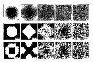
Figure 10 shows snapshots from a free expansion problem in which 16,384 particles, obeying the adiabatic equation of state $P\propto(\rho^{2}/2)$, expand to fill a space four times that of the initial compressed gas. This problem provides a resolution of Gibbs’ Paradox (that the entropy increases by $Nk\ln 4$ while Gibbs’ Liouville-based entropy, $-k\langle\ln f\rangle$, remains unchanged)b46 ; b47 . Detailed calculations show that the missing Liouville entropy is embodied in the kinetic-energy fluctuations. When these fluctuations are computed in a frame moving at the local average velocity,

$$v(r)=\sum_{j}w_{rj}v_{j}/\sum_{j}w_{rj}\ ,$$

the corresponding velocity fluctuations, $(\langle v^{2}\rangle-\langle v\rangle^{2})$ are just large enough to reproduce the thermal entropy. Most of the spatial equilibration occurs very quickly, in just a few sound traversal times. The contours of average density and average kinetic energy shown here illustrate another advantage of the SPAM averaging algorithm. The field variables are defined everywhere in the system, so that evaluating them on a regular grid, for plotting or analyses, is easy to do.

These local velocity fluctuations begin to be important only when the adiabatic expansion stretches all the way across the periodic confining box so that rightward-moving fluid collides with its leftward-moving periodic image and vice versa. The thermodynamic irreversibility of that collision process, reproduced in the thermal entropy, is just sufficient for the reversible dynamics to reflect the irreversible entropy increase, $Nk\ln 4$. A dense-fluid version of this dilute-gas free expansion problem appears in Bill’s lecture on shockwaves.

Figure 11: Equilibrated column for two system sizes. Five density contours are indicated by changes in plotting symbols. The arrows corresponding to the contours were calculated analytically from the continuum force-balance equation, $dP/dy=-\rho g$.

II.4 Collapse of a Fluid Column

Figure 12: Water Column collapse for three system sizes The computational time for this two-dimensional problem varies as the three-halves power of the number of particles used because corresponding times increase as $\sqrt{N}$ while the number of interactions varies as $N$.

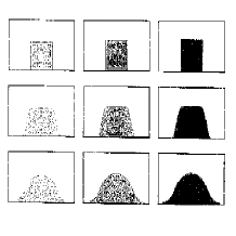
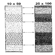
Figure 11 shows the distribution of smooth particles in an equilibrated periodic water column in a gravitational fieldb6 . Figure 12 shows snapshots from the subsequent collapse of the water column when the vertical periodic boundaries are released. Both the equilibration shown in Figure 11 and the collapse shown in Figure 12 use the simple equation of state $P=\rho^{3}-\rho^{2}$, chosen to give zero pressure at unit density. Here the gravitational field strength has been chosen to give a maximum density of 2 at the reflecting lower boundary. Initially, the vertical boundaries are periodic, preventing horizontal motion. After a brief equilibration period, the SPAM density profile can be compared to its analytic analog, derived by integrating the static version of the equation of motion:

$$dP/dy=-\rho g\ .$$

The arrows in Figure 11, computed from the analytic static density profile, show excellent agreement with the numerical SPAM simulation.

In smooth particle applied mechanics (SPAM) the boundary conditions are invariably the most difficult aspect of carrying out a simulationb6 ; b48 . Here we have used a simple mirror boundary condition at the bottom of the column and a periodic boundary at the sides, in the vertical direction. When the vertical periodic boundary constraint is released, rarefaction waves create a tensile region inside the falling column. By varying the size of the smooth particles the resolution of the motion can be enhanced, as Figure 12 shows. With “mirror boundaries”, elaborated in the next Section, more complicated situations can be treated. With mirrors there is an image particle across the boundary, opposite to each SPAM particle, with the mirror particle’s velocity and temperature both chosen to satisfy the corresponding boundary conditions.

Figure 13: Instantaneous temperature (below) and density (above) contours for the two-roll Rayleigh-Bénard problem. The stationary continuum solution (left) is compared to a SPAM snapshot with 5000 particles (right).

II.5 Rayleigh-Bénard Convection

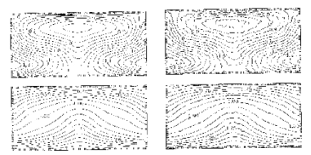
Figure 13 shows a typical snapshot for a slightly more complicated problem, the Rayleigh-Bénard problem, the convective flow of a compressible fluid in a gravitational field with the temperature specified at both the bottom (hot) and top (cold) boundaries. The velocities at both these boundaries must vanish, and can be imposed by using mirror particles resembling the image charges of electricity and magnetism. A particularly interesting aspect of the Rayleigh-Bénard problem is that multiple solutions of the continuum equations can coexist, for instance two rolls or four, with exactly the same boundary conditionsb42 ; b43 ; b44 ; b49 . Such work has been used to show that neither the entropy nor the entropy production rate allows one to choose “the solution”. Which solution is observed in practice can depend sensitively on the initial conditions. The Rayleigh-Bénard problem illustrates the need for local hydrodynamic averages describing the anisotropies of two- and three-dimensional flows.

SPAM provides an extremely useful interpolation method for generating twice-differentiable averages from particle data. In the following lecture this method will be used to analyze a dense-fluid molecular dynamics shockwave problem, where all of the thermomechanical variables make near-discontinuous changes linking an incoming cold state to an outgoing hot one. The continuous differentiable field variables provided by SPAM make it possible to analyze the relatively subtle nonlinear properties of such strongly nonequilibrium flow fields.

SPAM is a particularly promising field for graduate research. In addition to the many possible treatments of boundaries (including boundaries between different phases), the conservation of angular momentum (when shear stresses are present) and the tensile instability (where $w$ acts as an attractive rather than repulsive force) and the treatment of surface tension all merit more investigation. For a summary of the current State of the Art see our recent bookb6 .

III Tensor-Temperature Shockwaves via Molecular Dynamics

III.1 Introduction and Goals

Shockwaves are an ideal nonlinear nonequilibrium application of molecular dynamics. The boundary conditions are purely equilibrium and the gradients are quite large. The shockwave process is a practical method for obtaining high-pressure thermodynamic data. There are some paradoxical aspects too. Just as in the free expansion problem, time-reversible motion, with constant Gibbs’ entropy, describes a macroscopically irreversible process in which entropy increases. The increase is third-order in the compression, for weak shocksb50 . The shockwave problem is a compelling example of Loschmidt’s reversibility paradox.

We touch on all these aspects of the shockwave problem here. We generate and analyze the pair of shockwaves which results from the collision of two stress-free blocksb8 ; b9 . The blocks are given initial velocities just sufficient to compress the two cold blocks to a hot one, at twice the initial density. Further evolution of this atomistic system, with the initial kinetic energy of the blocks converted to internal energy, leads to a dense-fluid version of the free expansion problem discussed earlier for an adiabatic gas. Here we emphasize the dynamical reversibility and mechanical instability of this system, show the shortcomings of the usual Navier-Stokes-Fourier description of shockwaves, and introduce a two-temperature continuum model which describes the strong shockwave process quite well.

III.2 Shockwave Geometry

There is an excellent treatment of shockwaves in Chapter IX of Landau and Lifshitz’ “Fluid Mechanics” textb50 . A stationary shockwave, with steady flow in the $x$ direction, obeys three equations for the fluxes of mass, momentum, and energy derived from the three continuum equations expressing the conservation of mass, momentum, and energy:

$$\rho v=\rho_{C}u_{s}=\rho_{H}(u_{s}-u_{p})\ ;$$

$$P_{xx}+\rho v^{2}=P_{C}+\rho_{C}u_{s}^{2}=P_{H}+\rho_{H}(u_{s}-u_{p})^{2}\ ;$$

$$\rho v[e+(P_{xx}/\rho)+(v^{2}/2)]+Q_{x}=$$

$$[e+(P_{xx}/\rho)]_{C}+(u_{s}^{2}/2)=[e+(P_{xx}/\rho)]_{H}+(u_{s}-u_{p})^{2}/2\ .$$

Figure 14 illustrates the shockwave geometry in a special coordinate frame. In this frame the shockwave is stationary. Cold material enters from the left at the “shock speed” $u_{s}$ and hot material exits at the right, at speed $u_{s}-u_{p}$, where $u_{p}$ is the “particle” or “piston” velocity. The terminology comes from an alternative coordinate system, in which motionless cold material is compressed by a piston (moving at $u_{p}$), launching a shockwave (moving at $u_{s}$).

Eliminating the two speeds from the three conservation equations gives the Hugoniot equation,

$$e_{H}-e_{C}=(P_{H}+P_{C})(V_{C}-V_{H})/2\ ,$$

which relates the equilibrium pressures, volumes, and energies of the cold and hot states. Evidently purely equilibrium thermodynamic equation of state information can be obtained by applying the conservations laws to optical or electrical velocity measurements in the highly-nonequilibrium shockwave compression process. Ragan described the threefold compression of a variety of materials (using an atomic bomb explosion to provide the pressure) at pressures up to 60 Megabars, about 15 times the pressure at the center of the earthb51 .

Figure 14: Stationary shockwave in the comoving frame. Cold material enters at the left, with velocity $+u_{s}$, and is decelerated by the denser hotter material which exits at the right, with velocity $u_{s}-u_{p}$. It is in this coordinate frame that the fluxes given in the text are constant.

Figure 15: A series of snapshots showing the stability of a planar shockwave. Note that the decay of the initial sinewave profile is slightly underdamped. Here $Dt=2000dt$ is the time required for a shockwave to traverse the width shown here, 2000 Runge-Kutta timesteps with $dt=0.02/u_{s}\simeq 0.01$.

Figure 16: Snapshots near the beginning (upper) and end (lower) of an inelastic collision between two 400-particle blocks. The initial velocities, $\pm 0.965$, are just sufficient for a twofold compression of the cold material. The unit-mass particles interact with a short-ranged potential $(10/\pi)(1-r)^{3}$ and have an initial density $\sqrt{4/3}$.

Hoover carried out simulations of the shockwave compression process for a repulsive potential, $\phi(r)=r^{-12}$, in 1967b52 , but put off completing the project for several years, until computer storage capacity and execution speeds allowed for more accurate workb53 . Comparison of Klimenko and Dremin’s computer simulationsb18 using the Lennard-Jones potential, $\phi(r)=r^{-12}-2r^{-6}$, showed that relatively weak shockwaves (30 kilobars for argon, 1.5-fold compression) could be described quite wellb53 ; b54 with the three-dimensional Navier-Stokes equations, using Newtonian viscosity and Fourier heat conduction:

$$P=P_{eq}-\lambda\nabla\cdot v-\eta[\nabla v+\nabla v^{t}]\ ;$$

$$\lambda_{2D}=\eta_{v}-\eta\ ;\ \lambda_{3D}=\eta_{V}-(2/3)\eta\ ;$$

$$Q=-\kappa\nabla T\ .$$

Here $\lambda$ is the “second viscosity”, defined in such a way that the excess hydrostatic pressure due to a finite strain rate is $-\eta_{V}\nabla\cdot v$. The shear viscosity $\eta$ and heat conductivity $\kappa$ were determined independently using molecular dynamics simulations. The small scale of the wavesb54 , just a few atomic diameters, was welcomed by high-pressure experimentalists weary of arguing that their explosively-generated shockwaves measured equilibrium properties.

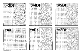
It is necessary to verify the one-dimensional nature of the waves too. It turns out that shockwaves do become planar very rapidly, at nearly the sound velocity. The rate at which sinusoidal perturbations are damped out has been used to determine the plastic viscosity of a variety of metals at high pressureb55 . Figure 15 shows the rapid approach to planarity of a dense-fluid shockwaveb9 .

Stronger shockwaves, where the bulk viscosity is more important (400 kilobars for argon, twofold compression), showed that the Navier-Stokes description needs improvement at higher pressures. In particular, within strong shockwaves temperature becomes a symmetric tensor, with $T_{xx}>>T_{yy}$, where $x$ is again the propagation direction. In addition, the Navier-Stokes-Fourier shockwidth, using linear transport coefficients, is too narrow. The tensor character of temperature in dilute-gas shockwaves had been carefully discussed in the 1950s by Mott-Smithb37 .

III.3 Analysis of Instantaneous Shockwave Profiles using SPAM Averaging

Data for systems with impulsive forces, like hard spheres, require both time and space averaging for a comparison with traditional continuum mechanics. Analyses of molecular dynamics data with continuous potentials need no time averaging, but still require a spatial smoothing operation to convert instantaneous particle data, $\{x,y,p_{x},p_{y}\}_{i}$, including $\{P,Q,T,e\}_{i}$, to equivalent continuous continuum profiles, $\{\rho(r,t),v(r,t),e(r,t),P(r,t),T(r,t),Q(r,t)\}$.

The potential parts of the virial-theorem and heat-theorem expressions for the pressure tensor P and the heat-flux vector Q,

$$PV=\sum_{i<j}F_{ij}r_{ij}+\sum_{i}(pp/mk)_{i}\ ;\$$

$$QV=\sum_{i<j}F_{ij}\cdot p_{ij}r_{ij}+\sum_{i}(ep/mk)_{i}\ ,\$$

can be apportioned in at least three “natural” ways between pairs of interacting particlesb7 ; b56 .

Consider the potential energy of two particles, $\phi(|r_{12}|)$. This contribution to the system’s energy can be split equally between the two particle locations, $r_{1}$ and $r_{2}$, or located at the midpoint between them, $(r_{1}+r_{2})/2$, or distributed uniformlyb56 along the line $r_{1}-r_{2}$ joining them. These three possibilities can be augmented considerably in systems with manybody forces between particles of different masses. It is fortunate that for the short-ranged forces we study here the differences among the three simpler approaches are numerically insignificant. Once a choice has been made, so as to define particle pressures and heat fluxes, these can in turn be used to define the corresponding continuum field variables at any location $r$ by using the weight-function approach of smooth particle applied mechanics:

$$P(r)\equiv\sum_{j}P_{j}w_{rj}/\sum_{j}w_{rj}\ ;\ Q(r)\equiv\sum_{j}Q_{j}w_{rj}/\sum_{j}w_{rj}\ .$$

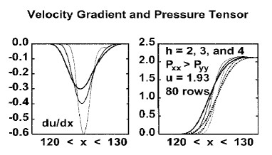
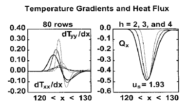
By using this approach our own simulations have characterized another constitutive complication of dense-fluid shockwaves – the time delays between [1] the maximum shear stress and the maximum strainrate and [2] the maximum heat flux and and the maxima of the two temperature gradients $(dT_{xx}/dx)$ and $(dT_{yy}/dx)$b8 ; b57 . The study of such delays goes back to Maxwell. The “Maxwell relaxation” of a viscoelastic fluid can be described by the modelb7 ; b8 ; b57 :

$$\sigma+\tau\dot{\sigma}=\eta\dot{\epsilon}\ .$$

so that stress reacts to a changing strainrate after a time of order $\tau$. Cattaneo considered the same effect for the propagation of heat. The phenomenological delays, found in the dynamical results, are a reminder that the irreversible nature of fluid mechanics is fundamentally different to the purely-reversible dynamics underlying it.

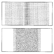
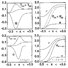
The irreversible shock process is particularly interesting from the pedagogical standpoint. The increase in entropy stems from the conversion of the fluid’s kinetic energy density, $\rho v^{2}/2$ to heat. To avoid the need for discussing the work done by moving pistons of Figure 14, we choose here to investigate shockwaves generated by symmetric collisions of two stressfree blocks, periodic in the direction parallel to the shockfront. The entropy increase is large here (a zero-temperature classical system has an entropy of minus infinity). Figure 16 shows two snapshots for a strong shockwave yielding twofold compression of the initial cold zero-pressure lattice. The mechanical and thermal variables in a strong dense-fluid shockwave are shown in Figure 17. In order to model these results two generalizations of traditional hydrodynamics need to be made: the tensor nature of temperature and the delayed response of stress and heat flux both need to be treated. A successful approach is described next.

Figure 17: Shock Thermal and Mechanical Profiles from molecular dynamics are shown at the top. Corresponding numerical solutions of the generalized continuum equations are shown at the bottom. This rough comparison suggests that the generalized equations can be fitted to particle simulations. The generalized equations use tensor temperature and apportion heat and work between the two temperatures $T_{xx}$ and $T_{yy}$. They also include delay times for shear stress, for heat flux, and for thermal equilibration.

Figure 18: Shear Stress lags behind the strainrate. The molecular dynamics gradients, using smooth-particle interpolation, are much more sensitive to the range of the weighting function than are the fluxes. The results here are shown for $h=2,3,4$, with line widths corresponding to $h$.

Figure 19: Heat Flux lags behind the temperature gradients. The molecular dynamics gradients, using smooth-particle interpolation, are much more sensitive to the range of the weighting function than are the fluxes. The results here are shown for $h=2,3,4$, with line widths corresponding to $h$.

III.4 Macroscopic Generalizations of the Navier-Stokes-Fourier Approach

By generalizing continuum mechanics to include tensor temperature and the time delays for stress and heat flux,

$$\sigma+\tau\dot{\sigma}=\eta\dot{\epsilon}\ ;\ Q+\tau\dot{Q}=-\kappa\nabla T\ ,$$

with an additional relaxation time describing the joint thermal equilibration of $T_{xx}$ and $T_{yy}$ to a common temperature $T_{H}$ the continuum and dynamical results can be made consistentb7 ; b8 ; b9 ; b37 ; b38 ; b40 . In doing this we partition the work done and the heat gained into separate longitudinal ($x$) and transverse ($y$) parts:

$$\rho\dot{T}_{xx}\propto-\alpha\nabla v:P-\beta\nabla\cdot Q+\rho(T_{yy}-T_{xx})/\tau\ ;\$$

$$\rho\dot{T}_{yy}\propto-(1-\alpha)\nabla v:P-(1-\beta)\nabla\cdot Q+\rho(T_{xx}-T_{yy})/\tau\ .$$

Solving the time-dependent continuum equations for such shockwave problems is not difficultb9 ; b42 . If all the spatial derivatives in the continuum equations are expressed as centered differences, with density defined in the center of a grid of cells, and all the other variables (velocity, energy, stress, heat flux, …) at the nodes defining the cell vertices, fourth-order Runge-Kutta integration converges nicely to solutions of the kind shown in Figure 17.

III.5 Shockwaves from Two Colliding Blocks are Nearly Reversible

To highlight the reversibility of the irreversible shockwave process let us consider the collision of two blocks of two-dimensional zero-pressure material, at a density of $\sqrt{4/3}$ (nearest-neighbor distance is unity, as is also the particle mass). Measurement of the equation of state with ordinary Newtonian mechanics, using the pair potential,

$$\phi(r<1)=(10/\pi)(1-r)^{3}\ ,$$

indicates (and simulation confirms) that the two velocities $u_{s}$ and $u_{p}$,

$$u_{s}=2u_{p}=1.930\ ,$$

correspond to twofold compression with a density change $\sqrt{4/3}\rightarrow 2\sqrt{4/3}$. To introduce a little chaos into the initial conditions random initial velocities, corresponding to a temperature $10^{-10}$ were chosen. Because the initial pressure is zero the conservation relations are as follows:

$$\rho v=\sqrt{4/3}\times 1.930=2.229\ ;$$

$$\ P_{xx}+\rho v^{2}=\sqrt{4/3}\times 1.930^{2}=4.301\ ;$$

$$\rho v[e+(P_{xx}/\rho)+\rho v^{2}/2)]+Q_{x}=\sqrt{4/3}\times 1.930^{3}/2=4.151\ .$$

Although the reversibility of the dynamics cannot be perfect, the shockwave propagates so rapidly that a visual inspection of the reversed dynamics shows no discrepancies over thousands of Runge-Kutta timesteps. To assess the mechanical instability of the shock compression process we explore the effects of small perturbations to the reversible dynamics in the following Sections. We begin by illustrating phase-space instabilityb26 ; b58 for a simpler problem, the harmonic chain.

III.6 Linear Growth Rates for a Harmonic Chain

Even the one-dimensional harmonic chain, though not chaotic, exhibits linear phase-volume growth in certain phase-space directions. Consider the equations of motion for a periodic chain incorporating an arbitrary scalefactor $s^{+2}$:

$$\{\ \dot{q}=ps^{+2}\ ;\ \dot{p}=(q_{+}-2q+q_{-})s^{-2}\ \}\ ;$$

the subscripts indicate nearest-neighbor particles to the left and right. The motion equations for a $2N$-dimensional perturbation vector $\delta=(\delta q,\delta p)$ follow by differentiation:

$$\{\ \delta\dot{q}=\delta ps^{+2}\ ;\ \delta\dot{p}=(\delta q_{+}-2\delta q+\delta q_{-})s^{-2}\ \}\ .$$

If we choose the length of the perturbation vector equal to unity, the logarithmic growth rate, $\Lambda=(d\ln\delta/dt)_{q,p}$, is a sum of the individual particle contributions:

$$\Lambda(\delta)=\sum[\delta q\delta p(s^{+2}-2s^{-2})+\delta p(\delta q_{+}+\delta q_{-})s^{-2}]\ .$$

For a large scale factor $s^{+2}$ it is evident that choosing equal components of the vector provides the maximum growth rate,

$$\{\delta q=\delta p=\sqrt{1/2N}\}\ \rightarrow\ \Lambda_{\rm max}=2^{-1}s^{+2}\ .$$

For $s^{2}$ small, rather than large, alternating signs give the largest growth rate, with

$$\{\ +\delta q_{\rm even}=+\delta p_{\rm odd}=-\delta q_{\rm odd}=-\delta p_{\rm even}\ \}\ ,$$

the growth rate is

$$\Lambda_{\rm max}=2^{+1}s^{-2}-2^{-1}s^{+2}\ .$$

The growth rate is $2^{-1/2}$ at the transition between the two regions, where $s^{2}\stackrel{{\scriptstyle<}}{{>}}2^{1/2}$.

These same growth-rate results can be found numerically by applying “singular value decomposition” to the dynamical matrix $D$b26 ; b58 . This analysis details the deformation of an infinitesimal phase-space hypersphere for a short time $dt$. During this time the hypersphere has its components $\delta q,\delta p$ changed by the equations of motion:

$$\delta\stackrel{{\scriptstyle dt}}{{\longrightarrow}}(I+Ddt)\cdot\delta\ ,$$

so that the growth and decay rates can be found from the diagonal elements of the singular value decomposition

$$I+Ddt=U\cdot W\cdot V^{t}\rightarrow\{\Lambda=(1/dt)\ln W\}\ .$$

Numerical evaluation gives the complete spectrum of the growth and decay rates. The maximum matches the analytic results given above. Although locally the growth rates $\{\Lambda(r,t)\}$ are nonzero, the harmonic chain is not at all chaotic and the long-time-averaged Lyapunov exponents $\{\lambda=\langle\lambda(r,t)\rangle\}$, all vanish. Let us now apply the concepts of phase-space growth rates $\{\Lambda\}$ and the Lyapunov exponents $\{\lambda\}$ to the shockwave problem.

III.7 Linear Instability in Many Body Systems, $\Lambda$ for Shockwaves

Figure 20: Phase-space Growth Rates $\{\Lambda\}$ during the collision of two 240-particle blocks of length 20. The collision leads to twofold compression of the original cold material at a time of order $20/1.93\simeq 10.4$. At time = 12 the velocities were reversed, so that the configurations at times 2, 4, and 6 correspond closely to those at 22, 20, and 18 respectively. Those particles making above average contributions to the largest phase-space growth direction are indicated with open circles. The fourth-order Runge-Kutta timestep is $dt=0.002$.

The time reversibility of the Hamiltonian equations of motion guarantees that any stationary situation shows both a long-time-averaged and a local symmetry between the forward and reversed directions of time. In such a case the $N$ nonzero time-averaged Lyapunov exponents as well as the local growth rates, obey the relations

$$\{\ \lambda_{N+1-k}+\lambda_{k}\}=0\ ;\ \{\ \Lambda_{N+1-k}+\Lambda_{k}\}=0\ .$$

The instantaneous Lyapunov exponents $\{\lambda(t)\}$ depend on the dynamical history, while the instantaneous diagonalized phase-space growth rates, which we indicate with $\Lambda(t)$ rather than $\lambda(t)$, do not.

The rates $\{\Lambda(t)\}$ for different directions in phase space can be calculated efficiently from the dynamical matrix $D$, by using singular value decomposition, just as we did for the harmonic chain:

$$D=\left(\begin{array}[]{cc}\partial\dot{q}/\partial q&\ \partial\dot{q}/\partial p\\ \partial\dot{p}/\partial q&\ \partial\dot{p}/\partial p\end{array}\right)=\left(\begin{array}[]{cc}0&\ 1/m\\ \partial F/\partial q&0\end{array}\right)\ .$$

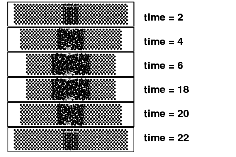
Here we analyze a 480-particle shockwave problem, the collision of two blocks with $x$ velocity components $\pm 0.965$. Figure 20 shows those particles making above-average contributions to the maximum phase-space growth rate at times 2, 4, and 6. At time 12 the particle velocities are all reversed, so that the configurations at times 22, 20 and 18 closely match those at times 2, 4, and 6. Generally there is six-figure agreement between the coordinates going forward in time and those in the reversed trajectory at corresponding times. Note this symmetry in Figure 20, where the most sensitive particles going forward and backward are exactly the same at corresponding times. The forward-backward agreement could be made perfect by following Levesque and Verlet’s suggestionb59 to use integer arithmetic in evaluating a time-reversible (even bit-reversible!) algorithm such as

$${\rm Int}[q_{t+dt}-2q_{t}+q_{t-dt}]={\rm Int}[F_{t}dt^{2}/m]\ {\rm or}$$

$${\rm Int}[q_{t+2dt}-q_{t+dt}-q_{t-dt}+q_{t-2dt}]={\rm Int}[(dt^{2}/4m)(5F_{t+dt}+2F_{t}+5F_{t-dt})]\ .$$

Evidently, as would be expected, from their definition, the point-function growth rates $\{\Lambda(r(t))\}$ can show no “arrow of time” distinguishing the backward trajectory from the forward one. We turn next to the Lyapunov exponents, which can and do show such an arrow.

III.8 Lyapunov Spectrum in a Strong Shockwave

Most manybody dynamics is Lyapunov unstable, in the sense that the length of the phase-space vector joining two nearby trajectories has a tendency to grow at a (time-dependent) rate $\lambda_{1}(t)$ (with the time-averaged result $\lambda_{1}\equiv\langle\lambda_{1}(t)\rangle>0$). Likewise, the area of a moving phase-space triangle, with its vertices at three nearby trajectories, grows at $\lambda_{1}(t)+\lambda_{2}(t)$, with a time-averaged rate $\lambda_{1}+\lambda_{2}$. The volume of a tetrahedron defined by four trajectories grows as $\lambda_{1}(t)+\lambda_{2}(t)+\lambda_{3}(t)$, and so on. By changing the scale factor linking coordinates to momenta – the $s^{+2}$ of the last Section – these exponents can be determined separately in either coordinate or momentum space.

Posch and Hoover, and independently Goldhirsch, Sulem, and Orszag, discovered a thought-provoking representation of local Lyapunov exponentsb60 ; b61 . If an array of Lagrange multipliers is chosen to propagate a comoving corotating orthonormal set of basis vectors centered on a phase space trajectory, the diagonal elements express local growth and decay rates. These are typically quite different (and unrelated) in the forward and backward directions of time.

Let us apply the Lyapunov spectrumb59 ; b60 ; b61 to the phase-space instability of a strong shockwave. Because the Lyapunov exponents, $\{\lambda(t)\}$, are evaluated so as to reflect only the past, times less than $t$, we expect to find that the Lyapunov vector corresponding to maximum growth soon becomes localized near the shock front. Starting out with randomly oriented vectors the time required for this localization is about 1/2. The time-linked disparities between the forward and backward motions suggest that the Lyapunov exponents can provide an “Arrow of Time” because the stability properties forward in time differ from those in the backward (reversed) direction of timeb62 .

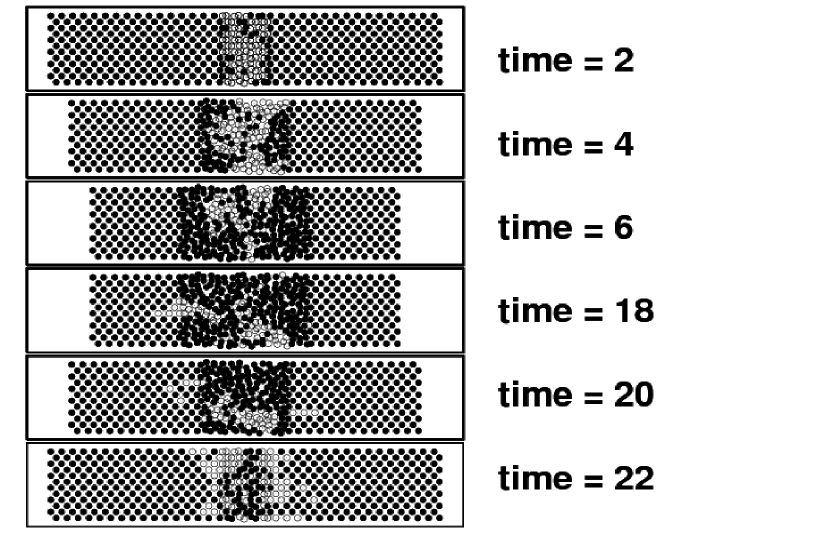
Figure 21 shows the particles making above-average contributions to the largest of the local Lyapunov exponents, $\lambda_{1}(t)$. There are many more of these particles than the few which contribute to the largest of the phase-space growth rates, $\Lambda_{1}(t)$. The shockwave simulation was run forward in time for 6000 timesteps, after which the velocities were reversed. The phase-space offset vectors, chosen randomly at time 0 and again at time 12, became localized near the shockfront at a time of order 0.5. The particles to which the motion is most sensitive, as described by the Lyapunov exponent $\lambda_{1}(t)$ are more localized in space in the forward direction of time than in the backward direction. Evidently the Lyapunov vectors are more useful than the vectors corresponding to local growth rates in describing the irreversibility of Hamiltonian systems.

Figure 21: Phase-space Growth Rates $\{\lambda\}$ during the collision of two similar blocks which lead to the twofold compression of the original cold material. At time = 12 the velocities were reversed, so that the configurations at times 2 and 4 correspond to those at 22 and 20, respectively. The particles making above average contributions to the largest Lyapunov exponent are indicated with open circles.

IV Conclusion

Particle dynamics, both NEMD and SPAM, provides a flexible approach to the simulation, representation, and analysis of nonequilibrium problems. The two particle methods are closely related, making it possible to infer constitutive relations directly from atomistic simulations. These useful tools provide opportunities for steady progress in understanding far-from-equilibrium states. It is our hope that these tools will become widely adopted.

V Acknowledgment

We thank Vitaly Kuzkin for encouraging our work on this review.

References

- (1) Wm. G. Hoover, Molecular Dynamics (Springer-Verlag, Berlin, 1986, available at the homepage http://williamhoover.info/MD.pdf).
- (2) Wm. G. Hoover, Computational Statistical Mechanics (Elsevier, Amsterdam, 1991, available at the homepage http://williamhoover.info/book.pdf).
- (3) D. J. Evans and G. P. Morriss, “Statistical Mechanics of NonEquilibrium Liquids”, (Academic Press, London, 1990).
- (4) L. B. Lucy, “A Numerical Approach to the Testing of the Fission Hypothesis”, The Astronomical Journal 82, 1013-1024 (1977).
- (5) R. A. Gingold and J. J. Monaghan, “Smoothed Particle Hydrodynamics: Theory and Application to Nonspherical Stars”, Monthly Notices of the Royal Astronomical Society 181, 375-389 (1977).
- (6) Wm. G. Hoover, Smooth Particle Applied Mechanics — The State of the Art (World Scientific Publishers, Singapore, 2006, available from the publisher at the publisher’s site http://www.worldscibooks.com/mathematics/6218.html).
- (7) Wm. G. Hoover and C. G. Hoover, “Shockwaves and Local Hydrodynamics; Failure of the Navier-Stokes Equations” [in New Trends in Statistical Physics, Festschrift in Honor of Leopoldo Garcí́a-Colín’s 80th Birthday Alfredo Macias and Leonardo Dagdug, Editors] (World Scientific, Singapore, 2010).
- (8) Wm. G. Hoover and C. G. Hoover, “Well-Posed Two-Temperature Constitutive Equations for Stable Dense Fluid Shockwaves using Molecular Dynamics and Generalizations of Navier-Stokes-Fourier Continuum Mechanics”, Physical Review E 81, 046302 (2010).
- (9) Wm. G. Hoover, C. G. Hoover, and F. J. Uribe, “Flexible Macroscopic Models for Dense-Fluid Shockwaves: Partitioning Heat and Work; Delaying Stress and Heat Flux; Two-Temperature Thermal Relaxation”, in Proceedings of Advanced Problems in Mechanics, Saint Petersburg, July 2010, available in arXiv 1005.1525 (2010).
- (10) E. Fermi, J. Pasta, and S. Ulam, “Studies of Nonlinear Problems I”, Los Alamos report LA-1940 (1955), in Collected Papers of Enrico Fermi, E. Segré, Editor, (University of Chicago Press, 1965).
- (11) J. L. Tuck and M. T. Menzel, “The Superperiod of the Nonlinear Weighted String (Fermi Pasta Ulam Problem)”, Advances in Mathematics 9, 399-407 (1972).
- (12) G. Benettin, “Ordered and Chaotic Motions in Dynamical Systems with Many Degrees of Freedom”, pages 15-40 in Molecular Dynamics Simulation of Statistical Mechanical Systems; Proceedings of the International School of Physics Enrico Fermi, Course XCVII, G. Ciccotti and W. G. Hoover, Editors (North-Holland, Amsterdam, 1986).
- (13) J. B. Gibson, A. N. Goland, M. Milgram, and G. H. Vineyard, “Dynamics of Radiation Damage”, Physical Review 120, 1229-1253 (1960).
- (14) W. W. Wood and J. D. Jacobson, “Preliminary Results from a Recalculation of the Monte Carlo Equation of State of Hard Spheres”, Journal of Chemical Physics 27, 1207-1208 (1957).
- (15) B. J. Alder and T. E. Wainwright, “Phase Transition for a Hard Sphere System”, Journal of Chemical Physics 27, 1208-1209 (1957).
- (16) J. A. Barker and D. Henderson, “What is ‘Liquid’? Understanding the States of Matter”, Reviews of Modern Physics 48, 587-671 (1976).
- (17) W. T. Ashurst and W. G. Hoover, “Argon Shear Viscosity via a Lennard-Jones Potential with Equilibrium and Nonequilibrium Molecular Dynamics”, Physical Review Letters 31, 206-208 (1973).
- (18) V. Y. Klimenko and A. N. Dremin, “Structure of a Shockwave Front in a Liquid”, in Detonatsiya, Chernokolovka, G. N. Breusov et alii, Editors (Akademia Nauk, Moscow, 1978), page 79-83.
- (19) D. Levesque, L. Verlet, and J. Kürkijarvi, “Computer ‘Experiments’ on Classical Fluids. IV. Transport Properties and Time Correlation Functions of the Lennard-Jones Liquid Near its Triple Point”, Physical Review A 7, 1690-1700 (1973).
- (20) L. V. Woodcock, “Isothermal Molecular Dynamics Calculations for Liquid Salts”, Chemical Physics Letters 10, 257-261 (1971).
- (21) S. Nosé, “Constant Temperature Molecular Dynamics Methods”, Progress of Theoretical Physics Supplement 103 (Molecular Dynamics Simulations, S. Nosé, Editor), 1-46 (1991).
- (22) W. G. Hoover, “Canonical Dynamics: Equilibrium Phase-Space Distributions”, Physical Review A 31, 1695-1697 (1985).
- (23) W. G. Hoover, “Mécanique de Nonéquilibre à la Californienne”, Physica A 240, 1-11 (1997).
- (24) G. D. Venneri and W. G. Hoover, “Simple Exact Test for Well-Known Molecular Dynamics Algorithms”. Journal of Computational Physics 73, 468-475 (1987).
- (25) H. J. C. Berendsen and W. G. van Gunsteren, “Practical Algorithms for Dynamics Simulations”, pages 43-65 in Molecular Dynamics Simulation of Statistical Mechanical Systems; Proceedings of the International School of Physics Enrico Fermi, Course XCVII, G. Ciccotti and W. G. Hoover, Editors (North-Holland, Amsterdam, 1986).
- (26) W. G. Hoover, C. G. Hoover, and F. Grond, “Phase-Space Growth Rates, Local Lyapunov Spectra, and Symmetry Breaking for Time-Reversible Dissipative Oscillators”, Communications in Nonlinear Science and Numerical Simulation 13, 1180-1193 (2008).
- (27) W. G. Hoover, C. G. Hoover, H. A. Posch, and J. A. Codelli, “The Second Law of Thermodynamics and MultiFractal Distribution Functions: Bin Counting, Pair Correlations, and the [definite failure of the] Kaplan-Yorke Conjecture”, Communications in Nonlinear Science and Numerical Simulation 12, 214-231 (2007).
- (28) B. L. Holian, W. G. Hoover, and H. A. Posch, “Resolution of Loschmidt’s Paradox: the Origin of Irreversible Behavior in Reversible Atomistic Dynamics”, Physical Review Letters, 59, 10-13 (1987).
- (29) J. D. Farmer, E. Ott, and J. A. Yorke, “The Dimension of Chaotic Attractors”, Physica D 7, 153-180 (1983).
- (30) B. Moran, W. G. Hoover, and S. Bestiale, “Diffusion in a Periodic Lorentz Gas” Journal of Statistical Physics 48, 709-726 (1987).
- (31) C. Dellago and W. G. Hoover, “Finite-Precision Stationary States At and Away from Equilibrium”, Physical Review E 62, 6275-6281 (2000).
- (32) D. J. Evans, E. G. D. Cohen, and G. P. Morriss, “Probability of Second Law Violations in Shearing Steady States”, Physical Review Letters 71, 2401-2404, and 3616 (1993).
- (33) C. Jarzynski, “Nonequilibrium Work Relations: Foundations and Applications”, The European Physics Journal B 64, 331-340 (2008).
- (34) W. G. Hoover, H. A. Posch, and C. G. Hoover, “Fractal Dimension of Steady Nonequilibrium Flows”, Chaos 2, 245-252 (1992).
- (35) W. G. Hoover, C. G. Hoover, and J. Petravic, “Simulation of Two- and Three-Dimensional Dense-Fluid Shear Flows via Nonequilibrium Molecular Dynamics: Comparison of Time-and-Space Averaged Stresses from Homogeneous Doll’s and s’lloD Shear Algorithms with Those from Boundary-Driven Shear”, Physical Review E 78, 046701 (2008).
- (36) Wm. G. Hoover and H. A. Posch, “Numerical Heat Conductivity in Smooth Particle Applied Mechanics”, Physical Review E 54, 5142-5145 (1996).
- (37) H. M. Mott-Smith, “The Solution of the Boltzmann Equation for a Shockwave”, Physical Review 82, 885-892 (1951).
- (38) K. Xu and E. Josyula, “Multiple Translational Temperature Model and its Shock Structure Solution”, Physical Review E 71, 056308 (2005).
- (39) O. Kum, Wm. G. Hoover, and C. G. Hoover, “Temperature Maxima in Stable Two-Dimensional Shockwaves”, Physical Review E 56, 462-465 (1997).
- (40) B. L. Holian and M. Mareschal, “Heat-Flow Equation Motivated by the Ideal-Gas Shockwave”, Physical Review E 82, 026707 (2010).
- (41) D. J. Evans, W. G. Hoover, B. H. Failor, B. Moran, and A. J. C. Ladd, “Nonequilibrium Molecular Dynamics via Gauss’ Principle of Least Constraint”, Physical Review A 28, 1016-1021 (1983).
- (42) A. Puhl, M. M. Mansour, and M. Mareschal, “Quantitative Comparison of Molecular Dynamics with Hydrodynamics in Rayleigh-Bénard Systems”, Physical Review A 40, 1999-2012 (1989).
- (43) V. M. Castillo, Wm. G. Hoover, and C. G. Hoover, “Coexisting Attractors in Compressible Rayleigh-Bénard Flow”, Physical Review E 55, 5546-5550 (1997).
- (44) C. Normand, Y. Pomeau, and M. G. Velarde, “Convective Instability: A Physicist’s Approach”, Review of Modern Physics 49, 581-624 (1977)
- (45) P. Español and P. Warren, “Statistical Mechanics of Dissipative Particle Dynamics”, Europhysics Letters 30, 191-196 (1995).
- (46) Wm. G. Hoover, H. A. Posch, V. M. Castillo, and C. G. Hoover, “Computer Simulation of Irreversible Expansions via Molecular Dynamics, Smooth Particle Applied Mechanics, Eulerian, and Lagrangian Continuum Mechanics”, Journal of Statistical Physics, 100, 313-326 (2000).
- (47) Wm. G. Hoover and C. G. Hoover, “SPAM-Based Recipes for Continuum Simulations”, Computing in Science and Engineering 3, 78-85 (2001).
- (48) O. Kum, Wm. G. Hoover, and C. G. Hoover, “Smooth-Particle Boundary Conditions”, Physical Review E, 68, 017701 (2003).
- (49) V. M. Castillo and Wm. G. Hoover, “Entropy Production and Lyapunov Instability at the Onset of Turbulent Convection”, Physical Review E 58, 7350-7354 (1998).
- (50) L. D. Landau and E. M. Lifshitz, Fluid Mechanics (Reed Elsevier, Oxford, 2000).
- (51) C. E. Ragan, III, “Shockwave Experiments at Threefold Compression”, Physical Review A 29, 1391-1402 (1984).
- (52) R. E. Duff, W. H. Gust, E. B. Royce, M. Ross, A. C. Mitchell, R. N. Keeler, and W. G. Hoover, “Shockwave Studies in Condensed Media” in the Proceedings of the 1967 Paris Symposium Behaviour of Dense Media Under High Dynamic Pressures (Gordon and Breach, New York, 1968).
- (53) B. L. Holian, W. G. Hoover, B. Moran, and G. K. Straub, “Shockwave Structure via Nonequilibrium Molecular Dynamics and Navier-Stokes Continuum Mechanics”, Physical Review A 22, 2798-2808 (1980).
- (54) W. G. Hoover, “Structure of a Shockwave Front in a Liquid”, Physical Review Letters 42, 1531-1542 (1979).
- (55) V. N. Mineev and A. V. Mineev, “Viscosity of Metals under Shock-Loading Conditions”, Supplement to Journal de Physique III, C3-583-585 (1997).
- (56) R. J. Hardy, “Formulas for Determining Local Properties in Molecular Dynamics Simulation: Shockwaves”, Journal of Chemical Physics 76, 622-628 (1982).
- (57) D. D. Joseph and L. Preziosi, “Heat Waves”, Reviews of Modern Physics 61, 41-73 (1989).
- (58) F. Grond, H. H. Diebner, S. Sahle, S. Fischer, and O. E. Rossler, “A Robust, Locally Interpretable Algorithm for Lyapunov Exponents”, Chaos, Solitons, and Fractals 16, 841-852 (2003).
- (59) Wm. G. Hoover, Time Reversibility, Computer Simulation, and Chaos (World Scientific, Singapore, 1999 and 2001).
- (60) W. G. Hoover and H. A. Posch, Direct Measurement of Equilibrium and Nonequilibrium Lyapunov Spectra”, Physics Letters A 123, 227-230 (1987).
- (61) I. Goldhirsch, P.-L. Sulem, and S. A. Orszag, “Stability and Lyapunov Stability of Dynamical Systems: a Differential Approach and a Numerical Method”, Physica 27D, 311-337 (1987).
- (62) Wm. G. Hoover, C. G. Hoover, and H. A. Posch, “Dynamical Instabilities, Manifolds, and Local Lyapunov Spectra Far From Equilibrium”, Computational Methods in Science and Technology 7, 55-65 (2001).