Rolling friction for hard cylinder and sphere on viscoelastic solid

Abstract

We calculate the friction force acting on a hard cylinder or spherical ball rolling on a flat surface of a viscoelastic solid. The rolling friction coefficient depends non-linearly on the normal load and the rolling velocity. For a cylinder rolling on a viscoelastic solid characterized by a single relaxation time Hunter has obtained an exact result for the rolling friction, and our result is in very good agreement with his result for this limiting case. The theoretical results are also in good agreement with experiments of Greenwood and Tabor. We suggest that measurements of rolling friction over a wide range of rolling velocities and temperatures may constitute an useful way to determine the viscoelastic modulus of rubber-like materials.

1 Introduction

Rubber friction is a topic of huge practical importance, e.g., for tires, rubber seals, wiper blades, conveyor belts and syringes Book ; Grosch ; Persson1 ; JPCM ; P3 ; theory1 ; theory2 ; theory3 ; theory4 ; theory5 ; theory6 ; wear ; Mofidi ; Creton . Many experiments have been performed with a hard spherical ball rolling on a flat rubber substrateTabor1 ; Tabor2 ; Varadi1 . Nearly the same friction force is observed during sliding as during rolling, assuming that the interface is lubricated and that the sliding velocity and fluid viscosity are such that a thin lubrication film is formed with a thickness much smaller than the indentation depth of the ball, but larger than the amplitude of the roughness on the surfacesTabor1 . The results of rolling friction experiments have often been analyzed using a very simple model of Greenwood and TaborTabor1 , which however contains a (unknown) factor $\alpha$, which represent the fraction of the input elastic energy lost as a result of the internal friction of the rubber. In this paper we present a very simple theory for the friction force acting on a hard cylinder or spherical ball rolling on a flat rubber surface. For a cylinder rolling on a viscoelastic solid characterized by a single relaxation time HunterHunter has obtained an exact result for the rolling friction, and our result is in very good agreement with his result for this limiting case.

2 Theory

Using the theory of elasticity (assuming an isotropic viscoelastic medium), one can calculate the displacement field $u_{i}$ on the surface $z=0$ in response to the surface stress distributions $\sigma_{i}=\sigma_{3i}$. Let us define the Fourier transform

$$u_{i}({\bf q},\omega)={1\over(2\pi)^{3}}\int d^{2}x\ dt\ u_{i}({\bf x},t){\rm e}^{-i({\bf q}\cdot{\bf x}-\omega t)}$$

and similar for $\sigma_{i}({\bf q},\omega)$. Here ${\bf x}=(x,y)$ and ${\bf q}=(q_{x},q_{y})$ are two-dimensional vectors. In Ref. Persson1 we have shown that

$${u}_{i}({\bf q},\omega)=M_{ij}({\bf q},\omega)\sigma_{j}({\bf q},\omega)$$

or, in matrix form,

$${\bf u}({\bf q},\omega)=M({\bf q},\omega){\bf\sigma}({\bf q},\omega)$$

where the matrix $M$ is given in Ref. Persson1 .

We now assume that $\mid\nabla u_{z}({\bf x})\mid<1$ and that the surface stress only acts in the $z$-direction so that

$$u_{z}({\bf q},\omega)=M_{zz}({\bf q},\omega){\bf\sigma}_{z}({\bf q},\omega).$$

Since in the present case $\omega$ is of order $vq$ (where $v$ is the sliding or rolling velocity) we get $\omega/c_{T}q=v/c_{T}<<1$ in most cases of practical interest, where $c_{\rm T}$ is the transverse sound velocity in the rubber. In this case (see Ref. Persson1 ):

$$\left(M_{zz}\right)^{-1}=-{Eq\over 2(1-\nu^{2})}.$$

It is interesting to note that if, instead of assuming that the surface stress act in the $z$-direction, we assume that the displacement ${\bf u}$ point along the $z$-direction, then

$$\sigma_{z}({\bf q},\omega)=\left(M^{-1}\right)_{zz}({\bf q},\omega)u_{z}({\bf q},\omega)$$

where in the limit $\omega/c_{T}q<<1$,

$$\left(M^{-1}\right)_{zz}=-{2Eq(1-\nu)\over(1+\nu)(3-4\nu)}$$

which differ from (2) only with respect to a factor $4(1-\nu)^{2}/(3-4\nu)$. For rubber-like materials ($\nu\approx 0.5$) this factor is of order unity. Hence, practically identical results are obtained independently of whether one assumes that the interfacial stress or displacement vector is perpendicular to the nominal contact surface. In reality, neither of these two assumptions hold strictly, but the result above indicate that the theory is not sensitive to this approximation.

Now, assume that

$$\sigma_{z}({\bf x},t)=\sigma_{z}({\bf x}-{\bf v}t)$$

then

$$\sigma_{z}({\bf q},\omega)={1\over(2\pi)^{3}}\int d^{2}xdt\ \sigma_{z}({\bf x}-{\bf v}t)\ {\rm e}^{-i({\bf q}\cdot{\bf x}-\omega t)}$$

$$=\delta(\omega-{\bf q}\cdot{\bf v})\ \sigma_{z}({\bf q})$$

where

$$\sigma_{z}({\bf q})={1\over(2\pi)^{2}}\int d^{2}x\ \sigma_{z}({\bf x}){\rm e}^{-i{\bf q}\cdot{\bf x}}$$

If $F_{\rm f}$ denote the friction force then the energy dissipated during the time period $t_{0}$ equals

$$\Delta E=F_{\rm f}vt_{0}.$$

But this energy can also be written as

$$\Delta E=\int d^{2}xdt\ \dot{\bf u}\cdot\sigma$$

$$=\left(2\pi\right)^{3}\int d^{2}qd\omega\ (-i\omega){\bf u}({\bf q},\omega)\cdot{\bf\sigma}(-{\bf q},-\omega)$$

where $\omega={\bf v}\cdot{\bf q}$. Substituting (1) in (5) and using (3) and that

$$[\delta(\omega-{\bf q}\cdot{\bf v})]^{2}=(t_{0}/2\pi)\ \delta(\omega-{\bf q}\cdot{\bf v}),$$

gives

$$\Delta E=\left(2\pi\right)^{2}t_{0}\int d^{2}q\ (-i\omega)$$

$$\times M_{zz}(-{\bf q},-\omega)\sigma_{z}({\bf q})\sigma_{z}(-{\bf q}).$$

Comparing this expression with (4) gives the friction force

$$F_{\rm f}={\left(2\pi\right)^{2}\over v}\int d^{2}q\ (-i\omega)\ M_{zz}(-{\bf q},-\omega)\sigma_{z}({\bf q})\sigma_{z}(-{\bf q}).$$

Since $F_{\rm f}$ is real and since $\sigma_{z}(-{\bf q})=\sigma^{*}_{z}({\bf q})$ we get

$$F_{\rm f}={\left(2\pi\right)^{2}\over v}\int d^{2}q\ \omega{\rm Im}M_{zz}(-{\bf q},-\omega)|\sigma_{z}({\bf q})|^{2}.$$

Using (2) we can also write

$$F_{\rm f}={2\left(2\pi\right)^{2}\over v}\int d^{2}q\ {\omega\over q}{\rm Im}{1\over E_{\rm eff}(\omega)}|\sigma_{z}({\bf q})|^{2}.$$

where $E_{\rm eff}=E/(1-\nu^{2})$. In principle, $\nu$ depends on frequency but the factor $1/(1-\nu^{2})$ varies from $4/3\approx 1.33$ for $\nu=0.5$ (rubbery region) to $\approx 1.19$ for $\nu=0.4$ (glassy region) and we can neglect the weak dependence on frequency. Within the assumptions given above, equation (6) is exact. Note that even if we use $\sigma_{z}({\bf q})$ calculated to zero order in ${\rm tan}\delta$, the friction force (6) will be correct to linear order in ${\rm tan}\delta$. We also note that the present approach is very general and flexible. For example, instead of a semi-infinite solid as assumed above one may be interested in a thin viscoelastic film on a hard flat substrate. In this case, (assuming slip-boundary conditions) the $M({\bf q},\omega)$-function which enter in (6a) is determined bytheory4 ; Carbon

$$M^{-1}=-{Eq\over 2(1-\nu^{2})}S$$

$$S={(3-4\nu){\rm cosh}(2qd)+2(qd)^{2}-4\nu(3-2v)+5\over(3-4\nu){\rm sinh}(2qd)-2qd}$$

Note that as $d\rightarrow\infty$, $S\rightarrow 1$ and the present result reduces to (2). Substituting this in (6a) gives the rolling friction for a sphere (or cylinder) on a thin rubber film adsorbed to a hard flat substrate. We now apply the theory to (a) a rigid cylinder and (b) a rigid sphere rolling on a semi-infinite viscoelastic solid.

2.1 Cylinder

Consider a hard cylinder (radius $R$ and length $L_{y}>>R$) rolling on a viscoelastic solid. The same result is obtained during sliding if one assume lubricated contact and if one can neglect the viscous energy dissipation in the lubrication film. As discussed above, when calculating the friction force to linear order in ${\rm tan}\delta$ we can neglect dissipation when calculating the contact pressure $\sigma_{z}(x)$ and assume that the stress is of the Hertz form. Thus if we introduce a coordinate system with the $y$-axis parallel to the cylinder axis and with the origin of the $x$-axis in the middle of the contact area (of width $2a$), then the contact stress for $-a<x<a$:

$$\sigma_{z}(x)={2f_{\rm N}\over\pi a}\left[1-\left({x\over a}\right)^{2}\right]^{1/2}$$

where $f_{\rm N}=F_{\rm N}/L_{y}$ the load per unit length of the cylinder. The half-width of the contact area in the Hertz contact theory is

$$a=\left({4f_{\rm N}R\over\pi E_{\rm eff}}\right)^{1/2}$$

where we take $E_{\rm eff}$ to be $|E_{\rm eff}(\omega)|$ with $\omega={\bf q}\cdot{\bf v}$. Now, note that

$$\int d^{2}x\left[1-\left({x\over a}\right)^{2}\right]^{1/2}e^{-i{\bf q}\cdot{\bf x}}$$

$$=2\pi\delta(q_{y})\int_{-a}^{a}dx\ \left[1-\left({x\over a}\right)^{2}\right]^{1/2}e^{-iq_{x}x}$$

$$=2\pi\delta(q_{y})a\int_{-1}^{1}dz\ \left[1-z^{2}\right]^{1/2}e^{-iq_{x}az}$$

$$=2\pi\delta(q_{y}){\pi\over q_{x}}J_{1}(aq_{x})$$

Using (7) and (9) gives

$$\sigma({\bf q})={f_{\rm N}\over\pi aq_{x}}\delta(q_{y})J_{1}(q_{x}a)$$

Note that this expression satisfies

$$(2\pi)^{2}\sigma({\bf q=0})=\int d^{2}x\ \sigma_{z}({\bf x})=F_{\rm N}$$

where we have used that $\delta(q_{y}=0)=L_{y}/2\pi$. Substituting (10) in (6b) dividing by $F_{\rm N}$, and using that

$$[\delta(q_{y})]^{2}=(L_{y}/2\pi)\delta(q_{y}),$$

gives the friction coefficient:

$$\mu={8f_{\rm N}\over\pi}\int_{0}^{\infty}dq_{x}\ {\rm Im}{1\over E_{\rm eff}(q_{x}v)}{1\over(aq_{x})^{2}}J_{1}^{2}(q_{x}a)$$

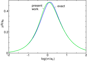
Figure 1: The friction coefficient (times the radius $R$ of the cylinder and divided by the half-width $a_{0}$ of the static contact region) as a function of $v\tau/a_{0}$, where $v$ is the rolling velocity, $\tau$ the rubber viscoelastic relaxation time (for $E_{1}/E_{0}=10$). We compare the exact result (blue curve) of HunterHunter with the prediction of Eq. (11) (green curve).

Let us now assume the simplest possible viscoelastic modulus characterized by a single relaxation time $\tau$:

$$E_{\rm eff}(\omega)={E_{1}(1-i\omega\tau)\over E_{1}/E_{0}-i\omega\tau}$$

where $E_{1}/E_{0}$ is the ratio between the high frequency and low frequency modulus. In Fig. 1 we show the friction coefficient (times the radius $R$ of the cylinder and divided by the half-width $a_{0}=a(v=0)$ of the static contact region) as a function of $v\tau/a_{0}$, where $v$ is the rolling velocity. We have assumed $E_{1}/E_{0}=10$. We compare the exact result (blue curve) of HunterHunter (the same result was obtained by GoryachevaGor ) with the prediction of Eq. (11) (green curve). Note that some distance away from the maximum the agreement between the two curve is perfect. This is expected because these regions correspond to small ${\rm tan}\delta$ where Eq. (11) should be essentially exact. Close to the maximum a small difference occur between the two curves, but from a practical point of view this is not important, since real rubber exhibit some non-linearity making any linear viscoelasticity theory only approximately valid anyhow.

At this point we empathize that (6) is basically exact, and if one could calculate the contact pressure $\sigma_{z}(x)$ [or rather the Fourier Transform $\sigma_{z}(q_{x})$] exactly, then (6) should give the exact result, e.g., the result of Hunter for the cylinder case, and assuming the simple viscoelastic modulus (12). Note that the contact pressure will not be symmetric around the midpoint when the dissipation in the rubber is included in the analysis. Still, to linear order in ${\rm tan}\delta$ one can neglect this effect [since (6) is explicitly already linear in ${\rm tan}\delta$], and the analysis above shows that this is a remarkable accurate approximation, which is an interesting result in its own right, and makes it possible to apply the theory to a wide set of problems.

2.2 Sphere

Consider a hard spherical (radius $R$) ball rolling on a viscoelastic solid. As discussed above, when calculating the friction force to linear order in ${\rm tan}\delta$ we can neglect dissipation when calculating the contact pressure $\sigma_{z}({\bf x})$ and assume that the stress is of the Hertz form:

$$\sigma_{z}({\bf x})={3F_{\rm N}\over 2\pi r_{c}^{2}}\left[1-\left({r\over r_{c}}\right)^{2}\right]^{1/2}$$

where $r=|{\bf x}|$ is the distance from the center of the contact area and $F_{\rm N}$ the load. The radius of the contact area in the Hertz contact theory is

$$r_{c}=\left({3F_{\rm N}R\over 4E_{\rm eff}}\right)^{1/3}$$

where we take $E_{\rm eff}$ to be $|E_{\rm eff}(\omega)|$ with $\omega={\bf q}\cdot{\bf v}$. Now, note that

$$\int d^{2}x\left[1-\left({r\over r_{c}}\right)^{2}\right]^{1/2}e^{-i{\bf q}\cdot{\bf x}}$$

$$=\int_{0}^{r_{c}}drr\left[1-\left({r\over r_{c}}\right)^{2}\right]^{1/2}\int_{0}^{2\pi}d\phi\ e^{-iqr{\rm cos}\phi}$$

$$=2\pi\int_{0}^{r_{c}}drr\left[1-\left({r\over r_{c}}\right)^{2}\right]^{1/2}J_{0}(qr)$$

$$=2\pi r_{c}^{2}\int_{0}^{1}dzz\left[1-z^{2}\right]^{1/2}J_{0}(qr_{c}z)$$

$$=2\pi r_{c}^{2}(qr_{c})^{-3}\left[{\rm sin}(qr_{c})-qr_{c}{\rm cos}(qr_{c})\right]$$

Using (13) and (15) gives

$$\sigma({\bf q})={3F_{\rm N}\over 4\pi^{2}}{1\over(qr_{c})^{3}}\left[{\rm sin}(qr_{c})-qr_{c}{\rm cos}(qr_{c})\right]$$

Note that this expression satisfies

$$(2\pi)^{2}\sigma({\bf q=0})=\int d^{2}x\ \sigma_{z}({\bf x})=F_{\rm N}$$

Substituting (16) in (6b) and dividing by $F_{\rm N}$ gives the friction coefficient:

$$\mu={9F_{\rm N}\over 2\pi^{2}}\int_{0}^{\infty}dqq\int_{0}^{2\pi}d\phi\ {\rm cos}\phi\ {\rm Im}{1\over E_{\rm eff}(qv{\rm cos}\phi)}$$

$$\times{1\over(qr_{c})^{6}}\left[{\rm sin}(qr_{c})-qr_{c}{\rm cos}(qr_{c})\right]^{2}$$

Eq. (17) is very general with no restriction on the viscoelastic properties of the rubber or on the sliding velocity $v$ (assuming that $v$ is small enough that the effect of frictional heating is negligible, and assuming $v<<c_{\rm T}$).

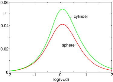
Figure 2: The friction coefficient as a function of $v\tau/d$, where $v$ is the rolling velocity, $\tau$ the rubber viscoelastic relaxation time, and $d=a_{0}$ for the cylinder (upper curve) or $d=r_{0}$ for the sphere (lower curve), rolling on a rubber substrate described by a simple viscoelastic model (see Eq. (12)). Here $a_{0}$ is half the width of the cylinder-substrate contact area and $r_{0}$ the radius of the contact region for the sphere, both in the limit of vanishing rolling velocity. In the calculation the radius of the sphere and of the cylinder are both $R=1\ {\rm cm}$ and the load was chosen so that the average contact pressure for the stationary contact was the same (equal to about $44\ {\rm kPa}$). For $E_{0}=1\ {\rm MPa}$ and $E_{1}/E_{0}=10$.

In Fig. 2 we show the rolling friction coefficient as a function of $v\tau/r_{0}$ for a sphere, and as a function of $v\tau/a_{0}$ for a cylinder. The ball has the radius $R=1\ {\rm cm}$ and is squeezed against a rubber surface with the load $F_{N}=0.15\ {\rm N}$ giving a static contact area with the radius $r_{0}=r_{c}(v=0)=0.10\ {\rm cm}$. The average contact pressure $p_{\rm a}=F_{N}/(\pi r_{0}^{2})=44.3\ {\rm kPa}$ is the same as for the cylinder case shown in the same figure. The cylinder has the radius $R=1\ {\rm cm}$ and is squeezed against a rubber surface with the load $f_{N}=100\ {\rm N/m}$ giving a static contact area with the width $a_{0}=0.11\ {\rm cm}$. The average contact pressure is $p_{\rm a}=f_{N}/(2a_{0})=44.3\ {\rm kPa}$. In the calculation we have used the viscoelastic modulus $E_{\rm eff}(\omega)$ given in Eq. (12). Note that at very low sliding velocities where the (average) contact pressure are the same the rolling frictions are nearly identical.

In figure 3 we show the maximum (as a function of the velocity $v$) of the rolling friction coefficients for a sphere and a cylinder, as a function of the average pressure in the static contact area. Note that $\mu$ varies nearly linearly with the (static) contact pressure, and using (8) and (14) it follows that the rolling friction coefficient $\mu\sim f_{\rm N}^{1/2}$ for the cylinder and $\mu\sim F_{\rm N}^{1/3}$ for the sphere.

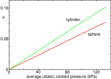
Figure 3: The maximum (as a function of the velocity $v$) of the rolling friction coefficients for a sphere and a cylinder, as a function of the average (static) contact pressure. For the same parameters as in Fig. 2.

Let us now consider the limiting case when the rolling velocity $v$ is so small that only the low-frequency viscoelastic modulus is relevant. We also assume that that $E(\omega)$ is given by (12). If $\omega\tau<<1$ for all relevant frequencies, we get ${\rm Re}E(\omega)\approx E(0)=E_{0}$ and ${\rm Im}E(\omega)\approx-\omega\tau E_{0}(1-E_{0}/E_{1})$. We also get $|E(\omega)|\approx E_{0}$. Substituting these results in (17) gives after some simplifications

$$\mu\approx{9I\over 2}{p_{\rm a}\over E_{0}}\left(1-{E_{0}\over E_{1}}\right){v\tau\over r_{0}}$$

where $p_{\rm a}=F_{\rm N}/(\pi r_{0}^{2})$ is the (average) static contact pressure, and where

$$I=\int_{0}^{\infty}d\xi\ \xi^{-4}\left({\rm sin}\xi-\xi{\rm cos}\xi\right)^{2}\approx 0.52$$

Note that $\mu\sim p_{\rm a}$ with is consistent with Fig. 3. If we define the frequency $\omega=v/r_{0}$ and note that in the present case ${\rm tan}\delta=(1-E_{0}/E_{1})\omega\tau$ we can write

$$\mu\approx{9I\over 2}{p_{\rm a}\over E_{0}}{\rm tan}\delta.$$

Since $9I/2\approx 2.34$ we get

$$\mu\approx 2.34{p_{\rm a}\over E_{0}}{\rm tan}\delta.$$

In Fig. 4 we compare this asymptotic (low velocity) result with the full theory [Eq. (17)]. For the limiting case studied above Greenwood and Tabor have shown that

$$\mu={9\pi\over 64}{p_{\rm a}\over E_{0}}\alpha,$$

where $\alpha$ is the fraction of the input elastic energy lost as a result of the internal damping of the rubber. Thus we can write

$$\alpha\approx 5.3{\rm tan}\delta.$$

Greenwood and Tabor analyzed rolling (and lubricated sliding) friction data using (20). They obtained the best fit to the experimental data by using an $\alpha$ which was almost a factor of two larger than obtained from cyclic (low frequency) simple uniaxial loading-unloading measurements of rubber strips, where the energy loss due to hysteresis was about 0.35 of the maximal elastic energy of deformation. For a linear viscoelastic solid the latter is given by $\pi{\rm tan}\delta$ (see Appendix A). Our theory predict that $\alpha$ (see (21)) is about $1.7$ times larger than $\pi{\rm tan}\delta$, and using this result gives very good agreement with the measured data presented in Ref. Tabor1 . The reason for why rolling friction experiments result in an $\alpha$-parameter which is larger than expected from uni-axial tension tests is related to the very different nature of the time-dependent deformations: a rubber volume element below a rolling sphere (or cylinder) undergoes, for some fraction of the interaction time, time-dependent deformations where the total elastic energy is nearly constant while the stress directions are changing and energy is being lost (see discussion in Ref. Tabor1 ; Green ).

Figure 4: The friction coefficient as a function of $v\tau/r_{0}$ for the sphere. The full line is using the full theory [Eq. (17)] and the dashed line using the asymptotic, low velocity, result (19). For the same parameters as in Fig. 2.

3 Rolling friction on rubber

We have calculated the rolling friction when a hard cylinder with radius $R=1\ {\rm cm}$ is rolling on a Styrene-Butadiene (SB) copolymer rubber surface at room temperature. The viscoelastic modulus of the rubber has been measured, and in Fig. 5 we show the loss tangent ${\rm tan}\delta={\rm Im}E(\omega)/{\rm Re}E(\omega)$ at $T=20\ {\rm C}$, as a function of frequency $\omega$ for an unfilled and filled SB-rubber. Note that ${\rm tan}\delta$ for the filled SB-rubber has a tail extending to very low frequencies. This correspond to relaxation processes in the rubber with very long relaxation times (see Fig. B.2 in JPCM ). This effect result from the increase in the activation barrier for polymer rearrangement processes for rubber molecules bound to (or close to) filler particles (in this case carbon particles).

The rolling friction coefficient is shown in Fig. 6 when the normal force per unit length is $10\ {\rm N/cm}$. The rolling friction exhibit a very strong temperature dependence given by the WLF shift factor $a_{T}$: reducing the temperature by $10\ {\rm C}$ result in a shift of the rolling friction curve towards lower velocities by approximately one decade. At low frequencies (or low rolling velocities) the unfilled SB rubber is elastically much softer than the filled rubber. Thus, the half width $a_{0}$ of the static Hertz contact region is $1.4\ {\rm mm}$ for the unfilled rubber but only $0.6\ {\rm mm}$ for the filled rubber. At high rolling velocities these values becomes much smaller owing to the stiffening of the effective elastic modulus at high frequencies. Note also that the rolling friction for filled SB rubber has a tail extending towards lower rolling velocities, which has the same origin as the tail in ${\rm tan}\delta$ towards lower frequencies, involving rubber molecules bound to the filler particles.

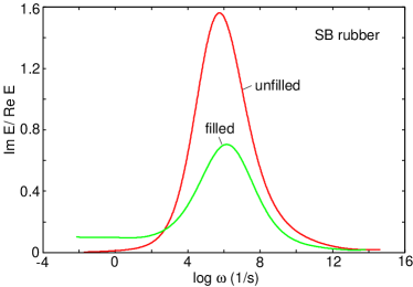
Figure 5: The loss tangent ${\rm tan}\delta={\rm Im}E(\omega)/{\rm Re}E(\omega)$ at $T=20\ {\rm C}$, as a function of frequency $\omega$ for an unfilled and filled SB rubber.

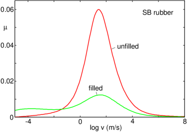
Figure 6: The rolling friction coefficient for a hard cylinder with radius $R=1{\rm cm}$ rolling on unfilled and filled SB rubber at $T=20\ {\rm C}$. The normal force on the cylinder per unit length is $10\ {\rm N/cm}$.

4 Discussion

Consider a rolling cylinder (or ball) in a reference frame where the center-of-mass velocity $v$ vanish. The rolling friction gives a moment $F_{\rm f}R$ at the center of the cylinder. Since the shear stress at the interface is assumed to vanish, this moment must arise from a contact pressure $\sigma_{z}(x)$ which is asymmetric around the center line of the cylinder. That is,

$$F_{\rm f}R=L_{y}\int dx\ x\sigma_{z}(x).$$

Thus the calculation of the rolling resistance gives information about how the centroid of the contact pressure shift away from the symmetry line $x=0$ due to the delayed response of the rubber caused by the internal friction of the rubber (characterized by the relaxation time $\tau$ in (12)). This information could in principle be used to improve the theoretical treatment given above, but since the simple theory we use seems to be very accurate, we will not consider this point further here.

The study presented above assumes that the adhesional interaction between the rubber and the hard ball can be neglected. Most rubber of engineering interest are strongly cross-linked and have fillers making them relative stiff and reducing the role of adhesion. Adhesion can also be removed (or reduced) by lubricating the interface or by adsorbing small inert solid particles on the rubber surface, e.g., talc. In these latter cases, the rolling and sliding friction may be nearly the same as indeed observed in some experimentsTabor1 . For very soft rubber and for clean surfaces, during rolling or sliding an opening (and a closing) crack will propagate at the interface, and associated with this may be very strong energy dissipation, which may dominate the rolling or sliding friction (see, e.g., Ref. Review .). We note finally that measurements of the rolling friction as a function of velocity $v$ and temperature $T$ may be a very useful way of determining the viscoelastic modulus $E(\omega)$, see Appendix B.

5 Summary and conclusion

We have presented a very general and flexible approach to calculate the rolling resistance of hard objects on viscoelastic solids. The theory can be applied to materials with arbitrary (e.g., measured) viscoelastic modulus $E(\omega)$. The theory can be applied to both spheres and cylinders rolling on semi-infinite viscoelastic solids, or on a thin viscoelastic film adsorbed on a rigid flat substrate, or even more complex situations for which the $M({\bf q},\omega)$-function can be calculated. For a cylinder rolling on a viscoelastic solid characterized by a single relaxation time $\tau$, Hunter has obtained an exact solution for the rolling resistance. We have shown that for this limiting case our theory gives almost the same as the result as obtained by Hunter. We have compared the rolling resistance of a sphere with that of a cylinder under similar circumstances. Measurements of the rolling friction as a function of velocity and temperature may be a very useful way of determining the viscoelastic modulus.

Acknowledgments

I thank J.A. Greenwood for drawing my attention to the work of S.C. Hunter and I.G. Goryacheva, and for supplying the numerical data for the blue curve in Fig. 1 (theory of Hunter). I also thank him and A. Nitzan for useful comments on the text. I thank A. Nitzan for the warm hospitality during a 2 weeks stay at Tel Aviv University where this work was done. I thank M. Klüppel for the (measured) viscoelastic modulus of the filled and unfilled SB-rubber. This work, as part of the European Science Foundation EUROCORES Program FANAS, was supported from funds by the DFG and the EC Sixth Framework Program, under contract N ERAS-CT-2003-980409.

Appendix A

Consider a strip of rubber in (slow) loading-unloading and assume that the strain $\varepsilon=\varepsilon_{0}{\rm sin}(\omega t)$, $0<t<t_{0}$ with $\omega t_{0}=\pi$. The energy dissipation (per unit volume)

$$U_{\rm diss}=\int_{0}^{t_{0}}dt\ \sigma\dot{\varepsilon}$$

$$=\int_{0}^{t_{0}}dt\ {\varepsilon_{0}\over 2i}\left(E(\omega)e^{i\omega t}-E(-\omega)e^{-i\omega t}\right)$$

$$\times{\varepsilon_{0}\over 2}\omega\left(e^{i\omega t}+e^{-i\omega t}\right)={1\over 2}\varepsilon_{0}^{2}\omega t_{0}{\rm Im}E(\omega)$$

We are considering very low frequencies so that the maximum elastic energy

$$U_{\rm el}\approx{1\over 2}E(0)\varepsilon_{0}^{2}\approx{1\over 2}{\rm Re}E(\omega)\varepsilon_{0}^{2}$$

Thus we get

$$\alpha={U_{\rm diss}\over U_{\rm el}}=\pi{{\rm Im}E(\omega)\over{\rm Re}E(\omega)}\approx\pi{\rm tan\delta}$$

Appendix B

The viscoelastic modulus $E(\omega)$ is a complex quantity and at first one may think that it impossible to determine both ${\rm Re}E(\omega)$ and ${\rm Im}E(\omega)$ from a knowledge of a single function $\mu(v)$ which depends on $E(\omega)={\rm Re}E(\omega)+i{\rm Im}E(\omega)$. However, $E(\omega)$ is (assumed to be) a causal linear response function so that ${\rm Im}E(\omega)$ can in fact be obtained from ${\rm Re}E(\omega)$ using a Kramer-Kronig relation. Thus we have one known function $\mu(v)$ and only one unknown function, e.g, ${\rm Re}E(\omega)$, and $E(\omega)$ can in principle be determined uniquely from $\mu(v)$. The best way of doing this is to note that $E(\omega)$ can be written as

$$E(\omega)=E_{1}-\int_{0}^{\infty}d\tau{H(\tau)\over 1-i\omega\tau}$$

In numerical calculations one may discretize the relation (B1) and it is usually enough to include $n\approx 15$ relaxation times $\tau_{k}$ with $\tau_{k+1}\approx 10\tau_{k}$. Thus we expand $E(\omega)$ on the form

$$E(\omega)=E_{1}-\sum_{k=1}^{n}{H_{k}\over 1-i\omega\tau_{k}}$$

where the $H_{k}$ and the relaxation times $\tau_{k}$ are real positive quantities. Next, form the quantity

$$V=\sum_{i}[\mu_{\rm meas}(v_{i})-\mu_{\rm theory}(v_{i};H_{1},...,H_{n})]^{2}g_{i}$$

where $g_{i}$ are suitable chosen weight coefficients (e.g., $g_{i}=1$) and where $v_{i}$ are the velocities for which the rolling friction has been measured. In (B3) we have indicated that the theory expression for the rolling friction coefficient depends on the numbers $H_{k}$. The determination of $H_{k}$ is a problem in multidimensional minimization of $V$, and can be performed using different methods, e.g., the Monte Carlo method or the Amoeba method, see Ref. Num .

References

- (1) B.N.J. Persson, Sliding Friction: Physical Principles and Applications, 2nd edn (2000) (Heidelberg, Springer).
- (2) K.A. Grosch, Proc. R. Soc. London, Ser. A274, 21 (1963).
- (3) B.N.J. Persson, J. Chem. Phys. 115, 3840 (2001).
- (4) B.N.J. Persson, J. Phys.: Condensed Matter 18, 7789 (2006).
- (5) G. Heinrich, M. Klüppel and T.A. Vilgis, Comp. Theor. Polym. Sci. 10, 53 (2000).
- (6) G. Heinrich and M. Klüppel, Wear 265, 1052 (2008).
- (7) B.N.J. Persson and A.I. Volokitin, Eur. Phys. J. E21, 69 (2006).
- (8) G. Carbone, B. Lorenz, B.N.J. Persson and A. Wohlers, Eur. Phys. J. E29, 275 (2009).
- (9) B.N.J. Persson, Surf. Sci. 401, 445 (1998).
- (10) A. Le Gal and M. Klüppel, J. Chem. Phys. 123, 014704 (2005).
- (11) B.N.J. Persson, J. Phys.: Condens. Matter 21, 485001 (2009).
- (12) M. Mofidi, B. Prakash, B.N.J. Persson and O. Albohr, J. Phys.: Condens. Matter 20, 085223 (2008).
- (13) See, e.g., B.N.J. Persson, O. Albohr, U. Tartaglino, A.I. Volokitin and E. Tosatti, J. Phys. Condens. Matter 17, R1 (2005).
- (14) B.N.J. Persson, O. Albohr, C. Creton and V. Peveri, J. Chem. Phys. 120, 8779 (2004)
- (15) J.A. Greenwood and D. Tabor, Proc. Roy. Soc. 71, 989 (1958).
- (16) J.A. Greenwood, Minshall and D. Tabor, Proc. Roy. Soc. (London) Serie A 250, 480 (1961).
- (17) D. Tabor, Phys. Educ. 29, 301 (1994).
- (18) D. Felhos, D. Xu, A.K. Schlarb, K. Varadi and T. Goda, Express Polymer Letters 2, 157 (2008).
- (19) S.C. Hunter, Trns. ASME, Series E, Journal of Applied Mechanics 28, 611 (1961).
- (20) G. Carbone and L. Mangialardi, The Journal of the Mechanics and Physics of Solids 56, 684 (2008)
- (21) B.N.J. Persson, O. Albohr, U. Tartaglino, G. Heinrich and H. Ueba, J. Phys. Condens. Matter 17, R1071 (2005).
- (22) I.G. Goryacheva, PMM 37, 925 (1973).
- (23) W.H. Press, S.A. Teukolsky, W.T. Vetterling and B.P. Flannery, Numerical Recipes, The Art of Scientific Computing, 3rd Edition, Cambridge University Press (2007).