The effective interaction hyperspherical harmonics method for non-local potentials

Abstract

A different formulation of the effective interaction hyperspherical harmonics (EIHH) method, suitable for non-local potentials, is presented. The EIHH method for local interactions is first shortly reviewed to point out the problems of an extension to non-local potentials. A viable solution is proposed and, as an application, results on the ground-state properties of 4- and 6-nucleon systems are presented. One finds a substantial acceleration in the convergence rate of the hyperspherical harmonics series. Perspectives for an application to scattering cross sections, via the Lorentz transform method are discussed.

1 Introduction

In solving the Schrödinger equation for the ground state of a many body system, via expansion techniques, one very often encounters the problem of convergence. In order to deal with this problem already several decades ago the notion of effective interaction (EI) has been introduced. The true EI is the operator that replaces the bare interaction when working in a finite model space, to give (at least) the same ground-state energy. In general it is an $A$-body operator. Therefore in the following we will denote it by $V^{[A]eff}$ and refer to it as to the total effective interaction. Finding $V^{[A]eff}$, however, is as difficult as solving the original problem, therefore over the years one has searched - more or less successfully - for the best approximations to it.

A different point of view has been introduced in the nineties with the No Core Shell Model (NCSM) [1]. The basic philosophy behind the NCSM success is that the EI is a partial effective interaction, tailored for the model space, however, constrained to coincide with the bare one, when enlarging the model space. This ensures that the energy will converge faster to the correct value. So, instead of pointing at getting the best approximation to the binding energy at a fixed model space, one points at reaching the converged solution as fast as possible, increasing the model space.

The same idea is behind the so called EIHH method [2]. The difference is that, instead of the harmonic oscillator basis (HO), the hyperspherical harmonics (HH) basis is used. There are some advantages in the EIHH approach: the EI is a function of the hyperradius parameter (a kind of “hyperlocal“ effective interaction) and in addition it is state dependent, resulting in a faster convergence, in the relevant quantum numbers, than in NCSM. The disadvantage is that working with the HH basis one does not take advantage of the well known versatility of the HO basis. In particular the straightforward application of the EIHH method to non-local potential presents some problems. In the following it will be shown what these problems are and how they can be overcome.

2 Short summary of the EIHH method for local potentials

2.1 Hyperspherical coordinates and hyperspherical harmonics

One characteristic of all the HH methods is that they respect translational invariance. In fact the hyper-spherical coordinates are defined by a transformation of the Jacobi coordinates ${\vec{\eta}}_{i}\,\,\,(i=1,2,...\,,A-1)$, in analogy with the spherical coordinates $(r,\hat{\Omega}_{2})$ of the 2-particle case.

Of the $(3A-3)$ coordinates the transformation retains the $(2A-2)$ Jacobi vector angles. The remaining $(A-1)$ coordinates are obtained generalizing the 3-dimensional space into a $(A-1)$-dimensional space, spanned by the modulus of the $(A-1)$ Jacobi vectors. Therefore, instead of the square radius $r^{2}$, that is the sum of the three squared coordinates, one has a square hyper-radius, $\rho^{2}$ that is the sum of the square modulus of the $(A-1)$ Jacobi vectors. The remaining $(A-2)$ coordinates are again angles and are the generalization of the definition of $\Omega_{2}$ in the 3-dimensional space to $\hat{\Omega}_{A-2}$ in the $(A-1)$-dimensional space. Summarizing, the hyper-spherical coordinates include one hyper-radius $\rho$ and $(3A-4)$ hyper-angles. We will denote all hyper-angles by $\hat{\Omega}_{A}$. So any function of the Jacobi coordinates $f(\vec{\eta}_{1},\vec{\eta}_{2},...\vec{\eta}_{A-1})$, when expressed in hyper-spherical coordinates becomes $f(\rho,\hat{\Omega}_{A})$.

The nice feature of these coordinates is that the kinetic energy operator of a many particle system takes a form in perfect analogy to the 2-particle 3-dimensional case: a $\rho$-dependent Laplacian and a hyper-centrifugal barrier, with a hyper-angular momentum operator $\hat{\bf K}$ that depends on all the hyper-angles. Therefore the translational invariant Hamiltonian for an $A$-particle system reads.

$$H^{[A]}=-\frac{1}{2m}\Delta_{\rho}+\frac{1}{2m}\frac{\hat{\bf K}_{A}^{2}}{\rho^{2}}+V^{[A]}(\rho,\hat{\Omega}_{A})\,,$$ (1)

The hyperspherical harmonics $\cal Y_{[\it K]}$ are eigenfunctions of $\hat{\bf K}$ with eigenvalues $K(K+3A-5)$. They constitute a useful basis where one can expand the $A$-particle wave function. It is as well useful to expand the hyperradial part in Laguerre polynomials $L^{\alpha}_{n}(\rho)$ so that one has

$$\Psi(\rho,\hat{\Omega}_{A})=\sum_{[K]n}C_{n[K]}L^{\alpha}_{n}(\rho){\cal Y}_{[K]}(\hat{\Omega}_{A})\,,$$ (2)

Of course the wave function must be complemented by the spin-isospin parts. The whole function must be antisymmetric. Therefore one needs to classify the hyperspherical harmonics according to the irreducible representations of the symmetry group of $A$ particles. This is a non trivial task, that, however, has been solved in [3].

2.2 Determination of an effective interaction for local potentials

In order to construct an EI we use the Lee-Suzuki similarity transformation [4]. This requires the definition of an $A$-particle model space $P$ ($Q$ denotes the rest of the whole Hilbert space, $P+Q=I$). For us $P$ will be spanned by all the $A$-body HH with $K\leq K_{max}$. In order to get the total EI the Lee-Suzuki method gives the recipe to get the similarity transformation that defines $H^{[A]eff}$, and therefore $V^{[A]eff}$. However, as already said above, we do not search for the total EI, but for a partial EI that is tailored for our HH model space and constrained to coincide with the bare one, only when enlarging the model space. This is naturally achieved in the following way:

• consider $\rho$ as a parameter;

• focus on a part of $H^{[A]}$, that we will call $H^{[2]}(\rho)$,

  $$H^{[2]}(\rho)=\frac{1}{2m}\frac{\hat{\bf K}_{A}^{2}}{\rho^{2}}+V_{A,A-1}(\rho,\hat{\Omega}_{A,A-1})\,.$$ (3)

  The term $V_{A,A-1}$ is just any of the pair potential terms in the Hamiltonian. For simplicity we choose the pair defining the ”simplest’ Jacobi coordinate $\vec{\eta}_{A,A-1}=\sqrt{\frac{1}{2}}(\vec{r}_{A}-\vec{r}_{A-1})$, since anyway we are working with antisymmetrized states. The eigenfunctions of $H^{[2]}(\rho)$ will live in a space that is contained in the $A$-body Hilbert space. There will be a $P_{2}$ contained in $P$ and a corresponding $Q_{2}$ contained in $Q$. Both of them are known since the eigenvalue problem for $H^{[2]}(\rho)$ can be easily solved, being a sort of 2-body problem “immersed in a medium” ($H^{[2]}$ depends on $\rho$!);

• apply the Lee-Suzuki similarity transformation to get the information residing in $Q_{2}$ into $P_{2}$ and obtain the EI $V^{[2]\,eff}(\rho)$;

• use this EI in the $P$ space;

• increase the $P$ space to convergence.

3 The effective interaction for non-local potentials

For non-local interactions one cannot proceed in the same way as described above. The reason is that for non-local interactions $V_{A,A-1}$ is a function of $(\rho,\hat{\Omega}_{A,A-1};\rho^{\prime},\hat{\Omega}^{\prime}_{A,A-1})$. If, as before the variable $\rho$ is considered a parameter, for fixed $\rho$ and $\rho^{\prime}$ one has $V_{A,A-1}(\rho,\hat{\Omega}_{A,A-1};\rho^{\prime},\hat{\Omega}^{\prime}_{A,A-1})\neq V_{A,A-1}(\rho,\hat{\Omega}^{\prime}_{A,A-1};\rho^{\prime},\hat{\Omega}_{A,A-1})$. This means that the potential is not hermitian!

A solution to overcome this problem is to start again from the full $H^{[A]}$, which for a non-local potential is written as

$$H^{[A]} = -\frac{1}{2m}\Delta_{\rho}+\frac{1}{2m}\frac{\hat{\bf K}_{A}^{2}}{\rho^{2}}+V^{[A]}(\rho,\hat{\Omega}_{A};\rho^{\prime},\hat{\Omega}^{\prime}_{A})$$ (4)

$$= -\frac{1}{2m}\Delta_{\rho}+\frac{1}{2m}\frac{\hat{\bf K}_{A}^{2}}{\rho^{2}}+V_{12}(\rho,\hat{\Omega}_{12};\rho^{\prime},\hat{\Omega}^{\prime}_{12})+...V_{A,A-1}(\rho,\hat{\Omega}_{A,A-1};\rho^{\prime},\hat{\Omega}^{\prime}_{A,A-1})\,,$$

and subtract and add a term that is local only in $\rho$, i.e. $V_{A,A-1}(\rho,\hat{\Omega}_{A,A-1};\rho,\hat{\Omega}^{\prime}_{A,A-1})$.

$$H^{[A]}= - \frac{1}{2m}\Delta_{\rho}+\frac{1}{2m}\frac{\hat{\bf K}_{A}^{2}}{\rho^{2}}+V^{[A]}(\rho,\hat{\Omega}_{A};\rho^{\prime},\hat{\Omega}^{\prime}_{A})$$

$$= - \frac{1}{2m}\Delta_{\rho}+\frac{1}{2m}\frac{\hat{\bf K}_{A}^{2}}{\rho^{2}}+V_{12}(\rho,\hat{\Omega}_{12};\rho^{\prime},\hat{\Omega}^{\prime}_{12})+...V_{A,A-1}(\rho,\hat{\Omega}_{A,A-1};\rho^{\prime},\hat{\Omega}^{\prime}_{A,A-1})-$$ (5)

$$- V_{12}(\rho,\hat{\Omega}_{12};\rho,\hat{\Omega}^{\prime}_{12})+V_{12}(\rho,\hat{\Omega}_{12};\rho,\hat{\Omega}^{\prime}_{12})-...+...$$

$$- V_{A,A-1}(\rho,\hat{\Omega}_{A,A-1};\rho,\hat{\Omega}^{\prime}_{A,A-1})+V_{A,A-1}(\rho,\hat{\Omega}_{A,A-1};\rho,\hat{\Omega}^{\prime}_{A,A-1})\,.$$

Table 1: Convergence of the HH expansion for the ⁴He ground-state energy (in MeV) and root-mean-square radius (in fm) with the bare and the effective non-local Idaho N³LO potential. Results with other methods are also given for comparison.

	Bare		Effective
$K_{\rm max}$	$<H>$	$\sqrt{<r^{2}>}$	$<H>$	$\sqrt{<r^{2}>}$
2	-3.507	1.935	-17.773	1.620
4	-13.356	1.523	-22.188	1.533
6	-20.135	1.446	-24.228	1.496
8	-23.721	1.451	-25.445	1.498
10	-24.617	1.470	-25.363	1.506
12	-25.115	1.491	-25.439	1.515
14	-25.259	1.501	-25.398	1.516
16	-25.310	1.509	-25.390	1.518
18	-25.359	1.513	-25.385	1.518
20	-25.370	1.515	-25.381	1.518
	-25.37(2)	1.515(4)	-25.38(1)	1.518(1)
HH [6]	-25.38	1.516
FY [6, 7]	-25.37	-
NCSM [8]	-25.39(1)	1.515(2)

From this expression one can single out a new $H^{[2]}(\rho)$ formed by the hypercentrifugal term and the last term

$$H^{[2]}(\rho)=\frac{1}{2m}\frac{\hat{\bf K}_{A}^{2}}{\rho^{2}}+V_{A,A-1}(\rho,\hat{\Omega}_{A,A-1};\rho,\hat{\Omega}^{\prime}_{A,A-1})\,.$$ (6)

In this quasi two-body Hamiltonian all non-local effects regarding the hyperspherical coordinates are incorporated, while the hyperradial part of the non-locality remains excluded.

Applying the Lee-Suzuki transformation to this new $H^{[2]}(\rho)$ one obtains $V^{[2]\,eff}_{[K][K^{\prime}]}(\rho)$. Then the effective non-local interaction is obtained by

$$v^{[2]\rm eff}_{[K_{A}],[K^{\prime}_{A}]}(\rho,\rho^{\prime})=v^{[2]}_{[K_{A}],[K^{\prime}_{A}]}(\rho,\rho^{\prime})+\delta(\rho-\rho^{\prime})\left(v^{[2]\rm eff}_{[K_{A}],[K^{\prime}_{A}]}(\rho,\rho)-v^{[2]}_{[K_{A}],[K^{\prime}_{A}]}(\rho,\rho)\right)\;.$$ (7)

The procedure described here is perfectly in line with the point of view stated above: all what is left out in the definition of the partial EI is recovered by increasing the model space $P$ up to convergence. In particular, since Eq. (7) represents a non-local HH effective interaction derived from the diagonal hyper-radial matrix element of $H^{[2]}$ in the position representation, it can be generalized to an arbitrary hyperradial basis. The question is which of this choices will lead to a better effective interaction, i.e. to a faster convergence of the HH expansion. This point has been studied in [5].

4 A test of the EIHH for non-local interaction

Here we present applications of the procedure described in the previous chapter to the case of 4- and 6-nucleon systems. In Table 1 we present results for ground-state energy and root-mean-square radius of ⁴He, obtained with the bare non-local Idaho N3LO potential [9] and with the corresponding effective interaction, using the hyperradial basis that leads to the best convergence [5]. (In order to work with this force we use a representation on a HO basis)

One sees that Kmax = 8 for ground-state energy and Kmax = 12 for the radius are already sufficient to obtain a convergence accuracy of less than 1%.

For $A=6$ nuclei the situation is illustrated in Fig. 1, for the ground-state energies of ⁶He and ⁶Li with the bare JISP16 nuclear force [10] and with the corresponding non-local EI. One notices that while it is not possible to obtain converged HH results for the bare interaction, the EI convergence is reached with a rather small effective interaction model space.

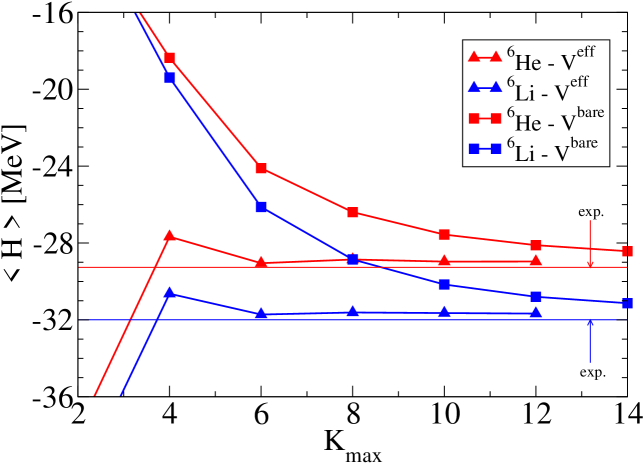
Figure 1: The ground-state energies of ⁶He and ⁶Li with the bare JISP16 nuclear force [10] and with the corresponding non-local effective interaction.

5 Perspectives for reaction cross sections

Calculating a reaction cross section ab initio is considered a much more difficult task than calculating binding energies or bound state observables in general. The reason is that in most cases reactions involve scattering states. The many-body scattering problem may lack a viable solution already for a very small number of constituents in the system.

The Lorentz Integral Transform method [11, 12] is able to overcome this longstanding stumbling block. In fact this approach reduces the scattering problem to a bound state-like problem. The essence of the method lays in finding the solution of a Schrödinger-like equation with a source $S$ that depends on the reaction one is study. In practice one has to solve

$$\left(\hat{H}-E_{0}-\sigma\right)|\tilde{\Psi}\rangle=S\,,$$ (8)

for many values of the real part $\sigma_{R}$ of the parameter $\sigma=\sigma_{R}+i\sigma_{I}$, and for a fixed value of its imaginary part $\sigma_{I}$, rigorously different from zero. It is just this last condition that ensures that the solution of Eq. (8) has bound-state boundary conditions. Therefore it can be found by any method suitable for bound states, like that described in this contribution.

The results found in the application of the present version of the EIHH method opens up a concrete possibility to study structure and reaction of a few/many-particle system within the same framework, also using potentials that are non-local, like the recent effective field theory potentials. This allows a critical review of different potential models, whose performances can be judged on a much larger set of observables.

References

References

-
[1]
Navrátil P and Barrett B R 1996 Phys. Rev. C
54 2986;
Navrátil P, Vary J P and Barrett B R 2000 Phys. Rev. Lett. 84 5728;
Navrátil P, Vary J P and Barrett B R 2000 Phys. Rev. C 62 054311 -
[2]
Barnea N, Leidemann W and Orlandini G 2000
Phys. Rev. C 61 054001;
Barnea N, Leidemann W and Orlandini G 2001 Nucl. Phys. A693 565 -
[3]
Barnea N and Novoselsky A 1997
Ann. Phys (N.Y.) 256 192;
Barnea N and Novoselsky A 1998 Phys. Rev. A 57 48 -
[4]
Suzuki K and Lee S Y 1980
Progr. Theor. Phys. 64 2091;
Suzuki K 1982 Progr. Theor. Phys. 68 246;
Suzuki K and Okamoto R 1983 Progr. Theor. Phys. 70 439 - [5] Barnea N, Leidemann W and Orlandini G 2010 Phys. Rev. C 81 064001
- [6] Viviani M, Girlanda L, Kievsky A, Marcucci L E and Rosati S 2007 Nucl. Phys. A790 46c
- [7] Nogga A, Kamada H, Glöckle W and Barrett B R 2002 Phys. Rev. C 65 054003
- [8] Gazit D, Quaglioni S and Navrátil P, 2009 Phys. Rev. Lett. 103 102502
- [9] Entem D R and Machleidt R 2001 Phys. Rev. C 68 041001
- [10] Shirokov A M, Vary J P, Mazur A and Weber T A 2007 Phys. Lett. B644 33
- [11] Efros V D, Leidemann W and Orlandini G 1994 Phys. Lett. B338 130
- [12] Efros V D, Leidemann W, Orlandini G and Barnea N 2007 J. Phys. G 34, R459