Searching for Dark Matter Signals in the Left-Right Symmetric Gauge Model with $CP$ Symmetry

Abstract

We investigate singlet scalar dark matter (DM) candidate in a left-right symmetric gauge model with two Higgs bidoublets (2HBDM) in which the stabilization of the DM particle is induced by the discrete symmetries $P$ and $CP$. According to the observed DM abundance, we predict the DM direct and indirect detection cross sections for the DM mass range from 10 GeV to 500 GeV. We show that the DM indirect detection cross section is not sensitive to the light Higgs mixing and Yukawa couplings except the resonance regions. The predicted spin-independent DM-nucleon elastic scattering cross section is found to be significantly dependent on the above two factors. Our results show that the future DM direct search experiments can cover the most parts of the allowed parameter space. The PAMELA antiproton data can only exclude two very narrow regions in the 2HBDM. It is very difficult to detect the DM direct or indirect signals in the resonance regions due to the Breit-Wigner resonance effect.

I Introduction

The existence of dark matter (DM) is by now well established from astrophysical observations DM . Together with the recent WMAP results, the cosmological observations have shown that the present Universe consists of about 73% dark energy, 23% dark matter, and 4% baryonic matter WMAP7 . In the standard model (SM) of particle physics, there is no cold DM candidate. Therefore, one has to extend the SM to account for the existence of DM. The DM candidate is often accompanied by some discrete symmetries to keep it stable, such as the R parity in supersymmetric (SUSY) models and KK parity in universal extra dimension models. Although the discrete symmetries are necessary for the DM stability, they may be introduced from different motivations DM .

In the left-right (LR) symmetric gauge model LRmodel ; Beall:1981ze ; Deshpande:1990ip with spontaneous $CP$ violation (SCPV), the $P$ and $CP$ symmetries are exact before the spontaneous symmetry breaking (SSB). In this case, it is possible that the discrete symmetries $P$ and $CP$ strongly constrain the scalar sector of the model and naturally give stable DM candidates. This possibility has not been emphasized in the literature, due to the fact that most of the popular models such as SM and SUSY violate $P$ maximally. In Ref. Guo:2008si , we have shown that the $P$ and $CP$ symmetries can give a stable DM candidate in an extension of a left-right symmetric gauge model with a singlet scalar field $S=(S_{\sigma}+iS_{D})/\sqrt{2}$. In this model, the $CP$ odd particle $S_{D}$ is stable even after the SSB, provided that it does not develop vacuum expectation value (VEV).

Without large fine-tuning, it is difficult to have a successful SCPV in the minimal left-right symmetric gauge model with only one Higgs bidoublet (1HBDM) Deshpande:1990ip ; Masiero:1981zd . This is because in the decoupling limit the predicted $CP$ violating quantity $\sin 2\beta\sim 0.1$ with $\beta$ being a $CP$ phase angle in the Cabibbo-Kobayashi-Maskawa (CKM) matrix is far below the experimentally measured value of $\sin 2\beta=0.671\pm 0.024$ from the two B-factories Ball:1999mb . In addition, the 1HBDM is also subject to strong phenomenological constraints from low energy flavor changing neutral current (FCNC) processes, especially the neutral kaon mixing which pushes the masses of the right-handed gauge bosons and some neutral Higgs bosons much above the TeV scale Mohapatra:1983ae . Motivated by the requirement of both spontaneous $P$ and $CP$ violations, we have considered the left-right symmetric gauge model with two Higgs bidoublets (2HBDM) Wu:2007kt . In the 2HBDM, the additional Higgs bidoublet modifies the Higgs potential so that the fine-tuning problem in the SCPV can be avoided, and the bounds from the FCNC processes can be relaxed. The extra Higgs bidoublet may also change the interferences among different contributions in the neutral meson mixings, and lower the bounds for the right-handed gauge boson masses not to be much higher than the TeV scale Wu:2007kt . Such a right-handed gauge boson can be searched at the LHC using the angular distributions of top quarks and the leptons from top quark decays Gopalakrishna:2010xm .

In Ref. Guo:2008si , we have shown that the discrete symmetries $P$ and $CP$ can be used to stabilize the DM candidate $S_{D}$ in the 1HBDM and 2HBDM with the SCPV. Using the observed DM abundance, we can constrain the parameter space and predict the spin-independent (SI) DM-nucleon elastic scattering cross section. For simplicity, we have only considered the case with no mixing among light neutral Higgs bosons in the 2HBDM and the dark matter is heavy. In this paper, we shall demonstrate in detail the mixing effect on the DM direct detection. Notice that several new DM annihilation channels can be derived, namely two DM particles may annihilate into a gauge boson and a Higgs boson. On the other hand, we are going to extend the DM mass range from $200\;{\rm GeV}\leq m_{D}\leq 500$ GeV to $10\;{\rm GeV}\leq m_{D}\leq 500$ GeV. As a consequence, one will meet several resonances in the 2HBDM. Therefore we shall consider the Breit-Wigner resonance effect for the determination of the DM relic density BW . In addition, we will also consider the DM indirect search in the 1HBDM and 2HBDM. The paper is organized as follows: In Section. II, we outline the main features of the 1HBDM and 2HBDM with a singlet scalar. In Sec. III and Sec. IV, we discuss the parameter space, the DM direct search and the DM indirect search in the 1HBDM and 2HBDM, respectively. Some conclusions are given in Sec. V.

II The left-right symmetric gauge model with a singlet scalar

We begin with a brief review of the 2HBDM described in Ref. Wu:2007kt . The model is a simple extension to the 1HBDM, which is based on the gauge group $SU(2)_{L}\otimes SU(2)_{R}\otimes U(1)_{B-L}$. The left- and right-handed fermions belong to $SU(2)_{L}$ and $SU(2)_{R}$ doublets, respectively. The Higgs sector contains two Higgs bidoublets $\phi$ (2,$2^{*}$,0), $\chi$ (2,$2^{*}$,0) and a left(right)-handed Higgs triplet $\Delta_{L(R)}$ (3(1),1(3),2) with the following flavor contents

$$\phi=\left(\begin{matrix}\phi_{1}^{0}&\phi_{2}^{+}\cr\phi_{1}^{-}&\phi_{2}^{0}\cr\end{matrix}\right),\;\chi=\left(\begin{matrix}\chi_{1}^{0}&\chi_{2}^{+}\cr\chi_{1}^{-}&\chi_{2}^{0}\cr\end{matrix}\right),\;\Delta_{L,R}=\left(\begin{matrix}\delta_{L,R}^{+}/\sqrt{2}&\delta_{L,R}^{++}\cr\delta_{L,R}^{0}&-\delta_{L,R}^{+}/\sqrt{2}\cr\end{matrix}\right).$$ (1)

The introduction of Higgs bidoublets $\phi$ and $\chi$ can account for the electroweak symmetry breaking and overcome the fine-tuning problem in generating the SCPV in the 1HBDM. Meanwhile it also relaxes the severe low energy phenomenological constraints Wu:2007kt . Motivated by the spontaneous $P$ and $CP$ violations, we require $P$ and $CP$ invariance of the Lagrangian, which strongly restricts the structure of the Higgs potential. The most general potential containing only the $\phi$ and $\Delta_{L,R}$ fields is given by

$$\mathcal{V}_{\phi\Delta} = -\mu_{1}^{2}\rm{Tr}(\phi^{\dagger}\phi)-\mu_{2}^{2}[\rm{Tr}(\tilde{\phi}^{\dagger}\phi)+\rm{Tr}(\tilde{\phi}\phi^{\dagger})]-\mu_{3}^{2}[\rm{Tr}(\Delta_{L}\Delta_{L}^{\dagger})+\rm{Tr}(\Delta_{R}\Delta_{R}^{\dagger})]$$ (2)

$$+\lambda_{1}[\rm{Tr}(\phi^{\dagger}\phi)]^{2}+\lambda_{2}\{[\rm{Tr}(\tilde{\phi}^{\dagger}\phi)]^{2}+[\rm{Tr}(\tilde{\phi}\phi^{\dagger})]^{2}\}+\lambda_{3}[\rm{Tr}(\tilde{\phi}^{\dagger}\phi)\rm{Tr}(\tilde{\phi}\phi^{\dagger})]$$

$$+\lambda_{4}\{\rm{Tr}(\phi^{\dagger}\phi)[\rm{Tr}(\tilde{\phi}^{\dagger}\phi)+\rm{Tr}(\tilde{\phi}\phi^{\dagger})]\}$$

$$+\rho_{1}\{[\rm{Tr}(\Delta_{L}\Delta_{L}^{\dagger})]^{2}+[\rm{Tr}(\Delta_{R}\Delta_{R}^{\dagger})]^{2}\}+\rho_{2}[\rm{Tr}(\Delta_{L}\Delta_{L})\rm{Tr}(\Delta_{L}^{\dagger}\Delta_{L}^{\dagger})+\rm{Tr}(\Delta_{R}\Delta_{R})\rm{Tr}(\Delta_{R}^{\dagger}\Delta_{R}^{\dagger})]$$

$$+\rho_{3}[\rm{Tr}(\Delta_{L}\Delta_{L}^{\dagger})\rm{Tr}(\Delta_{R}\Delta_{R}^{\dagger})]+\rho_{4}[\rm{Tr}(\Delta_{L}\Delta_{L})\rm{Tr}(\Delta_{R}^{\dagger}\Delta_{R}^{\dagger})+\rm{Tr}(\Delta_{L}^{\dagger}\Delta_{L}^{\dagger})\rm{Tr}(\Delta_{R}\Delta_{R})]$$

$$+\alpha_{1}\rm{Tr}(\phi^{\dagger}\phi)[\rm{Tr}(\Delta_{L}\Delta_{L}^{\dagger})+\rm{Tr}(\Delta_{R}\Delta_{R}^{\dagger})]+\alpha_{2}\rm{Tr}[(\tilde{\phi}^{\dagger}\phi)+(\tilde{\phi}\phi^{\dagger})]\rm{Tr}[(\Delta_{L}\Delta_{L}^{\dagger})+(\Delta_{R}\Delta_{R}^{\dagger})]$$

$$+\alpha_{3}[\rm{Tr}(\phi\phi^{\dagger}\Delta_{L}\Delta_{L}^{\dagger})+\rm{Tr}(\phi^{\dagger}\phi\Delta_{R}\Delta_{R}^{\dagger})]$$

$$+\beta_{1}[\rm{Tr}(\phi\Delta_{R}\phi^{\dagger}\Delta_{L}^{\dagger})+\rm{Tr}(\phi^{\dagger}\Delta_{L}\phi\Delta_{R}^{\dagger})]+\beta_{2}[\rm{Tr}(\tilde{\phi}\Delta_{R}\phi^{\dagger}\Delta_{L}^{\dagger})+\rm{Tr}(\tilde{\phi}^{\dagger}\Delta_{L}\phi\Delta_{R}^{\dagger})]$$

$$+\beta_{3}[\rm{Tr}(\phi\Delta_{R}\tilde{\phi}^{\dagger}\Delta_{L}^{\dagger})+\rm{Tr}(\phi^{\dagger}\Delta_{L}\tilde{\phi}\Delta_{R}^{\dagger})],$$

where the coefficients $\mu_{i}$, $\lambda_{i}$, $\rho_{i}$, $\alpha_{i}$ and $\beta_{i}$ in the potential are all real as all the terms are self-Hermitian. The Higgs potential $\mathcal{V}_{\chi\Delta}$ involving $\chi$ field can be obtained by the replacement $\chi\leftrightarrow\phi$ in Eq. (2). The mixing term $\mathcal{V}_{\chi\phi\Delta}$ can be obtained by replacing one of $\phi$ by $\chi$ in all the possible ways in Eq. (2). In order to simplify the discussion, we shall first consider the 1HBDM which already contains the main features of the complete model. Then we postpone the discussions on the $\chi$ contributions into Section IV.

After the SSB, the Higgs multiplets obtain nonzero VEVs

$$\langle\phi_{1,2}^{0}\rangle=\frac{\kappa_{1,2}}{\sqrt{2}}\;\mbox{ and }\;\langle\delta_{L,R}^{0}\rangle=\frac{v_{L,R}}{\sqrt{2}}\;,$$ (3)

where $\kappa_{1}$, $\kappa_{2}$, $v_{L}$ and $v_{R}$ are in general complex, and $\kappa\equiv\sqrt{|\kappa_{1}|^{2}+|\kappa_{2}|^{2}}\approx 246$ GeV represents the electroweak symmetry breaking scale. Due to the freedom of gauge symmetry transformation, one can take $\kappa_{1}$ and $v_{R}$ to be real. To avoid the fine-tuning problem of fermion masses, we require $v_{L}\simeq 0$ and $\kappa_{2}\ll\kappa_{1}$. The value of $v_{R}$ sets the scale of left-right symmetry breaking which is directly linked to the right-handed gauge boson masses. $v_{R}$ is subjected to strong constraints from the $K$, $B$ meson mixings Mohapatra:1983ae ; Ball:1999mb ; Beall:1981ze as well as low energy electroweak interactions Barenboim:1996nd ; Langacker:1989xa . The kaon mass difference and the indirect $CP$ violation quantity $\epsilon_{K}$ set a bound for $v_{R}$ around $10$ TeV Barenboim:1996nd ; Pospelov:1996fq .

	$P$	$CP$		$P$	$CP$		$P$	$CP$
$\phi$	$\phi^{\dagger}$	$\phi^{*}$	$S+S^{*}$	+	+	$S-S^{*}$	+	-
$\chi$	$\chi^{\dagger}$	$\chi^{*}$	$SS^{*}$	+	+	Tr($\phi^{{\dagger}}\phi$)	+	+
$\Delta_{L(R)}$	$\Delta_{R(L)}$	$\Delta_{L(R)}^{*}$	Tr($\phi^{{\dagger}}\tilde{\phi}+\tilde{\phi}^{{\dagger}}\phi$)	+	+	Tr($\phi^{{\dagger}}\tilde{\phi}-\tilde{\phi}^{{\dagger}}\phi$)	-	-
$S$	$S$	$S^{*}$	Tr($\Delta_{L}^{{\dagger}}\Delta_{L}+\Delta_{R}^{{\dagger}}\Delta_{R}$)	+	+	Tr($\Delta_{L}^{{\dagger}}\Delta_{L}-\Delta_{R}^{{\dagger}}\Delta_{R}$)	-	+

Table 1: The $P$ and $CP$ transformation properties of the Higgs particles and their gauge-invariant combinations. The “+” and “-” denote even and odd, respectively.

In our model, the $P$ and $CP$ symmetries have been required to be exactly conserved before the SSB, thus the discrete symmetries $P$ and $CP$ can be used to stabilize the DM candidate. In the framework of 2HBDM with a complex singlet scalar $S=(S_{\sigma}+iS_{D})/\sqrt{2}$, we have considered this possibility in Ref. Guo:2008si . The $P$ and $CP$ transformation properties of the Higgs particles and their gauge-invariant combinations have been shown in Table 1. It is clear that the odd powers of $(S-S^{*})$ are forbidden by the $P$ and $CP$ symmetries. Therefore $S_{D}$ is a stable particle and can be the DM candidate when the VEV $v_{\sigma}/\sqrt{2}$ of $S$ is real. Although $P$ and $CP$ are both broken after the SSB, there is a $CP$ type $Z_{2}$ discrete symmetry on $S_{D}$ remaining in the singlet sector. This discrete symmetry is induced from the original $CP$ symmetry. We have checked that the $P$ and $CP$ transformation rules for $S$ defined in Table 1 is actually the only possible way for the implementation of the DM candidate.

For the annihilation cross section of approximately weak strength, we expect that the DM mass is in the range of a few GeV and a few hundred GeV. However, the mass $m_{D}$ of $S_{D}$ is related to the LR symmetry breaking scale $v_{R}\sim 10$ TeV. To have a possible light DM mass, we may consider an approximate global $U(1)$ symmetry on $S$, i.e. $S\to e^{i\delta}S$. Then the $P$ and $CP$ invariant Higgs potential involving the singlet $S$ is given by

$$\mathcal{V}_{S} = -\mu_{D}^{2}SS^{*}+\lambda_{D}(SS^{*})^{2}+\sum_{i=1}^{3}\lambda_{i,D}SS^{*}O_{i}-\frac{m_{D}^{2}}{4}(S-S^{*})^{2}\;,$$ (4)

where $O_{1}={\rm{Tr}}(\phi^{{\dagger}}\phi)$, $O_{2}={\rm{Tr}}(\phi^{{\dagger}}\tilde{\phi}+\tilde{\phi}^{{\dagger}}\phi)$ and $O_{3}={\rm{Tr}}(\Delta_{L}^{{\dagger}}\Delta_{L}+\Delta_{R}^{{\dagger}}\Delta_{R})$. Only the last term explicitly violates $U(1)$ symmetry. After the SSB, $S$ obtains a real VEV $v_{\sigma}/\sqrt{2}$. Then one can straightly derive

$$\mathcal{V}_{S}=\frac{\lambda_{D}}{4}[(S_{\sigma}^{2}+2v_{\sigma}S_{\sigma}+S_{D}^{2})^{2}-v_{\sigma}^{4}]+\sum_{i=1}^{3}\frac{\lambda_{i,D}}{2}(S_{\sigma}^{2}+2v_{\sigma}S_{\sigma}+v_{\sigma}^{2}+S_{D}^{2})(O_{i}-\langle O_{i}\rangle)+\frac{m_{D}^{2}}{2}S_{D}^{2}\,,$$ (5)

where we have used the minimization condition $\mu_{D}^{2}=\lambda_{D}v_{\sigma}^{2}+\sum_{i}\lambda_{i,D}\langle O_{i}\rangle$ from the singlet $S_{\sigma}$ to eliminate the parameter $\mu_{D}$. The terms proportional to odd powers of $S_{D}$ are absent in Eq. (5) which implies $S_{D}$ can only be produced by pairs. Notice that the mass term of $S_{D}$ should be absent with an exact global $U(1)$ symmetry. As discussed in Ref. Guo:2008si , the explicit breaking of this $U(1)$ symmetry can explain the naturalness of a light DM mass $m_{D}$, but it does not destroy the stability of the DM candidate $S_{D}$.

Particles	Mass2	Particles	Mass2
$h^{0}=\phi_{1}^{0r}$	$m_{h^{0}}^{2}=2\lambda_{1}\kappa^{2}$	$H_{2}^{\pm}=\phi_{2}^{\pm}$	$m_{H_{2}^{\pm}}^{2}=\frac{1}{2}\alpha_{3}v_{R}^{2}$
$H_{1}^{0}=\phi_{2}^{0r}$	$m_{H_{1}^{0}}^{2}=\frac{1}{2}\alpha_{3}v_{R}^{2}$	$H_{R}^{\pm\pm}=\delta_{R}^{\pm\pm}$	$m_{H_{R}^{\pm\pm}}^{2}=2\rho_{2}v_{R}^{2}$
$A_{1}^{0}=-\phi_{2}^{0i}$	$m_{A_{1}^{0}}^{2}=\frac{1}{2}\alpha_{3}v_{R}^{2}$	$H_{L}^{\pm}=\delta_{L}^{\pm}$	$m_{H_{L}^{\pm}}^{2}=\frac{1}{2}(\rho_{3}-2\rho_{1})v_{R}^{2}$
$H_{2}^{0}=\delta_{R}^{0r}$	$m_{H_{2}^{0}}^{2}=2\rho_{1}v_{R}^{2}$	$H_{L}^{\pm\pm}=\delta_{L}^{\pm\pm}$	$m_{H_{L}^{\pm\pm}}^{2}=\frac{1}{2}(\rho_{3}-2\rho_{1})v_{R}^{2}$
$H_{3}^{0}=\delta_{L}^{0r}$	$m_{H_{3}^{0}}^{2}=\frac{1}{2}(\rho_{3}-2\rho_{1})v_{R}^{2}$	$A_{L}^{0}=\delta_{L}^{0i}$	$m_{A_{L}^{0}}^{2}=\frac{1}{2}(\rho_{3}-2\rho_{1})v_{R}^{2}$
$Z_{1}$	$m_{Z_{1}}^{2}=m_{W_{1}}^{2}\sec^{2}\theta_{W}$	$W_{1}^{\pm}=W_{L}^{\pm}$	$m_{W_{1}}^{2}=g^{2}\kappa^{2}/4$
$Z_{2}$	$m_{Z_{2}}^{2}=\frac{g^{2}v_{R}^{2}\cos^{2}\theta_{W}}{\cos 2\theta_{W}}$	$W_{2}^{\pm}=W_{R}^{\pm}$	$m_{W_{2}}^{2}=g^{2}v_{R}^{2}/2$

Table 2: The mass spectrum for the Higgs and gauge bosons in the left-right symmetric gauge model with one Higgs bidoublet in the limit $v_{L}\simeq 0$ and $\kappa_{2}\ll\kappa_{1}$. $\phi^{0r}_{i}$ and $\phi^{0i}_{i}$ stand for real and imaginary components of $\phi^{0}_{i}=(\phi^{0r}_{i}+i\phi^{0i}_{i})/\sqrt{2}$, respectively. The gauge boson $Z_{1}(W_{1})$ corresponds to the $Z(W)$ boson in the SM.

The terms $2v_{\sigma}S_{\sigma}O_{i}$ in Eq. (5) indicate that $S_{\sigma}$ will mix with the Higgs bosons ${\phi_{1}^{0r}}$, ${\phi_{2}^{0r}}$, ${\delta_{L}^{0r}}$ and ${\delta_{R}^{0r}}$. The relevant mass matrix elements are given by

$$M^{2}_{\sigma}=2\lambda_{D}v_{\sigma}^{2}\,,M^{2}_{\sigma\phi_{1}^{0r}}=\lambda_{1,D}\kappa v_{\sigma}\,,M^{2}_{\sigma\phi_{2}^{0r}}=2\lambda_{2,D}\kappa v_{\sigma}\,,M^{2}_{\sigma\delta_{L}^{0r}}=\lambda_{3,D}v_{\sigma}v_{L}\,,M^{2}_{\sigma\delta_{R}^{0r}}=\lambda_{3,D}v_{\sigma}v_{R}\;.$$ (6)

For simplicity here we require $v_{\sigma}>v_{R}\sim 10\;{\rm TeV}\gg\kappa$ which means the mixing angles between $S_{\sigma}$ and the above four neutral Higgs bosons are small. The terms $v_{\sigma}^{2}O_{i}$ in Eq. (5) do not change the minimization condition forms for $\phi$ and $\Delta_{L(R)}$. This is because these terms only change the overall coefficients $\mu_{1}$, $\mu_{2}$ and $\mu_{3}$ in Eq. (2). Hence the mass matrixes of the Higgs multiplets $\phi$ and $\Delta_{L,R}$ remain the same as that in the 1HBDM in Refs. Deshpande:1990ip ; Duka:1999uc , which also indicates that the additional potential term $\mathcal{V}_{S}$ in Eq. (5) does not help in resolving the fine-tuning problem. Due to $v_{L}\simeq 0$ and $\kappa_{2}\ll\kappa_{1}$, the mass eigenstates for the Higgs bidoublet and triplets approximately coincide with the corresponding flavor eigenstates. The mass spectrum for the Higgs and gauge bosons is listed in Table 2. There is only one light SM-like Higgs $h^{0}$ from the real part of $\phi^{0}_{1}$. The masses of all the other scalars are set by $v_{R}$ which can be very heavy. From the Lagrangian in Eq. (5) one can easily obtain the interaction terms among the scalars. Some of the relevant cubic and quartic scalar interaction vertexes are listed in Table 3.

Interaction	Vertex	Interaction	Vertex	Interaction	Vertex	Interaction	Vertex
$S_{D}S_{D}S_{\sigma}S_{\sigma}$	$-i2\lambda_{D}$	$S_{D}S_{D}h^{0}$	$-i\lambda_{1,D}\kappa$	$S_{D}S_{D}S_{\sigma}$	$-i2\lambda_{D}v_{\sigma}$	$S_{D}S_{D}H_{2}^{0}$	$-i\lambda_{3,D}v_{R}$
$S_{D}S_{D}HH^{*}$	$-i\lambda_{1,D}$	$S_{\sigma}S_{\sigma}h^{0}$	$-i\lambda_{1,D}\kappa$	$HH^{*}S_{\sigma}$	$-i\lambda_{1,D}v_{\sigma}$	$S_{\sigma}S_{\sigma}H_{2}^{0}$	$-i\lambda_{3,D}v_{R}$
$S_{D}S_{D}h^{0}H_{1}^{0}$	$-i2\lambda_{2,D}$	$S_{D}S_{D}H_{1}^{0}$	$-i2\lambda_{2,D}\kappa$	$h^{0}H_{1}^{0}S_{\sigma}$	$-i2\lambda_{2,D}v_{\sigma}$	$S_{\sigma}S_{\sigma}S_{\sigma}$	$-i6\lambda_{D}v_{\sigma}$
$S_{D}S_{D}\Delta\Delta^{*}$	$-i\lambda_{3,D}$	$S_{\sigma}S_{\sigma}H_{1}^{0}$	$-i2\lambda_{2,D}\kappa$	$\Delta\Delta^{*}S_{\sigma}$	$-i\lambda_{3,D}v_{\sigma}$	$h^{0}h^{0}H^{0}_{2}$	$-i\alpha_{1}v_{R}$

Table 3: The cubic and quartic scalar vertexes among Higgs singlets and multiplets, where $HH^{*}$ stands for any states of $\left(h^{0}h^{0},H_{1}^{0}H_{1}^{0},A_{1}^{0}A_{1}^{0},H_{2}^{+}H_{2}^{-}\right)$ and $\Delta\Delta^{*}$ stands for any states of $\left(H_{L}^{0}H_{L}^{0},A_{L}^{0}A_{L}^{0},H_{L}^{+}H_{L}^{-},H_{L}^{++}H_{L}^{--},H_{2}^{0}H_{2}^{0},H_{R}^{++}H_{R}^{--}\right)$.

III Dark matter signal in the 1HBDM

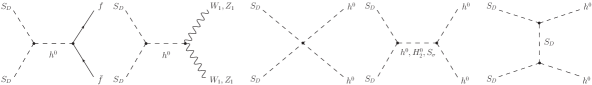
Figure 1: Feynman diagrams for the DM annihilation in the 1HBDM.

As discussed in Sec. II, an approximate global $U(1)$ symmetry on $S$ can naturally lead to a light DM mass $m_{D}$. Here we focus on $10\;{\rm GeV}\leq m_{D}\leq 500$ GeV. Considering the case $v_{\sigma}>v_{R}\sim 10\;{\rm TeV}\gg\kappa$, one may find that most of scalar bosons in Table 2 are very heavy except the SM-like one $h^{0}$. In this case, the possible annihilation products are $h^{0}h^{0}$, $W_{1}W_{1}/Z_{1}Z_{1}$ and fermion pairs $f\bar{f}$ as shown in Fig. 1. For $s$-channel annihilation processes, the intermediate particles may be $h^{0}$, $H_{1}^{0}$, $H_{2}^{0}$ and $H_{3}^{0}$. Because of $v_{L}\simeq 0$, one may neglect the $H_{3}^{0}$ case. In addition, the $H^{0}_{1}$ contribution is also negligible as $m_{H_{1}^{0}}\gg m_{h^{0}}$. For the $f\bar{f}$ annihilation process, the main contribution comes from the $h^{0}$ exchange diagram. This is because $H^{0}_{2}$ dominantly couples to the very heavy right-handed Majorana neutrinos (the corresponding annihilation process is kinematically forbidden). For the $W_{1}W_{1}/Z_{1}Z_{1}$ processes, the diagram involving $H^{0}_{2}$ is suppressed by $m_{H_{2}^{0}}\gg m_{h^{0}}$. Notice that $S_{\sigma}$ may be the intermediate particle for the $h^{0}h^{0}$ case. It is clear that the dominant annihilation processes in Fig. 1 are the same as that in the minimal extension of SM with a real gauge singlet scalar when $m_{D}<m_{h^{0}}$ McDonald . In the 1HBDM, the DM annihilation cross sections $\hat{\sigma}=4E_{1}E_{2}\sigma v$ ($E_{1}$ and $E_{2}$ are the energies of two incoming DM particles) for different annihilation channels have the following forms:

$$\LARGE\hat{\sigma}_{f\bar{f}} = \frac{\lambda_{1,D}^{2}m_{f}^{2}}{4\pi}\frac{1}{(s-m_{h^{0}}^{2})^{2}+m_{h^{0}}^{2}\Gamma_{h^{0}}^{2}}\frac{(s-4m_{f}^{2})^{1.5}}{\sqrt{s}},$$ (7)

$$\hat{\sigma}_{Z_{1}Z_{1}} = \frac{\lambda_{1,D}^{2}}{16\pi}\frac{s^{2}}{(s-m_{h^{0}}^{2})^{2}+m_{h^{0}}^{2}\Gamma_{h^{0}}^{2}}\sqrt{1-\frac{4m_{Z_{1}}^{2}}{s}}\left(1-\frac{4m_{Z_{1}}^{2}}{s}+\frac{12m_{Z_{1}}^{4}}{s^{2}}\right),$$ (8)

$$\hat{\sigma}_{W_{1}W_{1}} = \frac{\lambda_{1,D}^{2}}{8\pi}\frac{s^{2}}{(s-m_{h^{0}}^{2})^{2}+m_{h^{0}}^{2}\Gamma_{h^{0}}^{2}}\sqrt{1-\frac{4m_{W_{1}}^{2}}{s}}\left(1-\frac{4m_{W_{1}}^{2}}{s}+\frac{12m_{W_{1}}^{4}}{s^{2}}\right),$$ (9)

$$\hat{\sigma}_{h^{0}h^{0}} = \frac{\lambda_{1,D}^{2}}{16\pi}\sqrt{1-\frac{4m_{h^{0}}^{2}}{s}}\left[G_{1}^{2}-\frac{8\lambda_{1,D}\kappa^{2}}{s-2m_{h^{0}}^{2}}G_{1}F(\xi_{h^{0}})+\frac{8\lambda_{1,D}^{2}\kappa^{4}}{(s-2m_{h^{0}}^{2})^{2}}\left(\frac{1}{1-\xi_{h^{0}}^{2}}+F(\xi_{h^{0}})\right)\right],$$ (10)

where $s$ is the squared center-of-mass energy modify . The quantity $F$ is defined as $F(\xi_{h^{0}})\equiv\mbox{arctanh}(\xi_{h^{0}})/\xi_{h^{0}}$ with $\xi_{h^{0}}=\sqrt{s-4m_{D}^{2}}\sqrt{s-4m_{h^{0}}^{2}}/(s-2m_{h^{0}}^{2})$. The Higgs decay width $\Gamma_{h^{0}}$ and $G_{1}$ are given by

$$\Gamma_{h^{0}} = \frac{\sum m_{f}^{2}}{8\pi\kappa^{2}}\frac{(m_{h^{0}}^{2}-4m_{f}^{2})^{1.5}}{m_{h^{0}}^{2}}+\frac{m_{h^{0}}^{3}}{16\pi\kappa^{2}}\sqrt{1-\frac{4m_{W_{1}}^{2}}{m_{h^{0}}^{2}}}\left(1-\frac{4m_{W_{1}}^{2}}{m_{h^{0}}^{2}}+\frac{12m_{W_{1}}^{4}}{m_{h^{0}}^{4}}\right)$$

$$+\frac{m_{h^{0}}^{3}}{32\pi\kappa^{2}}\sqrt{1-\frac{4m_{Z_{1}}^{2}}{m_{h^{0}}^{2}}}\left(1-\frac{4m_{Z_{1}}^{2}}{m_{h^{0}}^{2}}+\frac{12m_{Z_{1}}^{4}}{m_{h^{0}}^{4}}\right)+\frac{\lambda_{1,D}^{2}\kappa^{2}}{32\pi}\frac{\sqrt{m_{h^{0}}^{2}-4m_{D}^{2}}}{m_{h^{0}}^{2}}\;,$$

$$G_{1} = 1+\frac{3m_{h^{0}}^{2}}{s-m_{h^{0}}^{2}}+\frac{\alpha_{1}\lambda_{3,D}v_{R}^{2}}{s-m_{H_{2}^{0}}^{2}}\frac{1}{\lambda_{1,D}}+\frac{m_{\sigma}^{2}}{s-m_{\sigma}^{2}}\;.$$ (11)

From Eqs. (7-11) seven unknown parameters enter the expression of total annihilation cross section, namely, $m_{h^{0}}$, $m_{D}$, $\lambda_{1,D}$, $\alpha_{1}\lambda_{3,D}$, $m_{\sigma}^{2}$, $m_{H_{2}^{0}}^{2}$ and $v_{R}$. For the mass of SM-like Higgs, we take $m_{h^{0}}=120$ GeV in the following parts. In fact, one may neglect the squared center-of-mass energy $s$ in the terms $s-m_{H_{2}^{0}}^{2}$ and $s-m_{\sigma}^{2}$ since the masses of $s_{\sigma}$ and $H^{0}_{2}$ are around $v_{R}$. In a good approximation, we find that only three independent parameters

$$m_{D},\lambda_{1,D}\;{\rm and}\;\lambda_{R}\equiv\alpha_{1}\lambda_{3,D}/(2\rho_{1})$$ (12)

are relevant to our numerical analysis. Here we have used $m_{H_{2}^{0}}^{2}=2\rho_{1}v_{R}^{2}$ as it is shown in Table 2.

III.1 Constraints from the DM relic density

In order to obtain the correct DM abundance, one should resolve the following Boltzmann equation KOLB :

$$\frac{dY}{dx}=-\frac{x\;{\bf s}(x)}{H}\langle\sigma v\rangle(Y^{2}-Y_{EQ}^{2})\;,$$ (13)

where $Y\equiv n/{\bf s}(x)$ denotes the DM number density. The entropy density ${\bf s}(x)$ and the Hubble parameter $H$ evaluated at $x=1$ are given by

$${\bf s}(x)=\frac{2\pi^{2}g_{*}}{45}\frac{m_{D}^{3}}{x^{3}}\;,\;H=\sqrt{\frac{4\pi^{3}g_{*}}{45}}\frac{m_{D}^{2}}{M_{\rm PL}}\;,$$ (14)

where $M_{\rm PL}\simeq 1.22\times 10^{19}$ GeV is the Planck energy. $g_{*}$ is the total number of effectively relativistic degrees of freedom. The numerical results of $g_{*}$ have been presented in Ref. APP . Here we take the QCD phase transition temperature to be 150 MeV. The thermal average of the annihilation cross section times the relative velocity $\langle\sigma v\rangle$ is a key quantity in the determination of the DM cosmic relic abundance. We adopt the usual single-integral formula for $\langle\sigma v\rangle$ Edsjo:1997bg :

$$\langle\sigma v\rangle=\frac{1}{n_{EQ}^{2}}\frac{m_{D}}{64\pi^{4}x}\int_{4m_{D}^{2}}^{\infty}\hat{\sigma}(s)\sqrt{s}K_{1}(\frac{x\sqrt{s}}{m_{D}})ds\;,$$ (15)

with

$$n_{EQ}=\frac{g_{i}}{2\pi^{2}}\frac{m_{D}^{3}}{x}K_{2}(x)\;,\;\hat{\sigma}(s)=\hat{\sigma}\;g_{i}^{2}\;\sqrt{1-\frac{4m_{D}^{2}}{s}}\;,$$ (16)

where $K_{1}(x)$ and $K_{2}(x)$ are the modified Bessel functions. $x\equiv m_{D}/T$ and $g_{i}=1$ is the internal degrees of freedom for the scalar dark matter $S_{D}$. In terms of the annihilation cross section $\hat{\sigma}$ in Eqs. (7-10), one can numerically calculate the thermally averaged annihilation cross section $\langle\sigma v\rangle$. Finally, we may obtain the DM relic density $\Omega_{D}h^{2}=2.74\times 10^{8}\;Y_{0}\;m_{D}/{\rm GeV}$ by use of the result $Y_{0}$ of the integration of Eq. (13).

When the DM mass $m_{D}$ is larger than the mass of top quark, one will not meet the resonance BW and threshold Threshold effects in our model. Thus we use the approximate formulas to calculate the DM relic density for $200\,{\rm GeV}\leq m_{D}\leq 500\,{\rm GeV}$. In this case, $\langle\sigma v\rangle$ can be expanded in powers of relative velocity and $x^{-1}$ for nonrelativistic gases. To the first order $\langle\sigma v\rangle\simeq\sigma_{0}x^{-n}$, where $n=0(1)$ for $s(p)$-wave annihilation process KOLB . The approximate formula for $\langle\sigma v\rangle$ is given by Srednicki:1988ce

$$\langle\sigma v\rangle=\sigma_{0}x^{-n}=\frac{1}{m_{D}^{2}}\left[\omega-\frac{3}{2}(2\omega-\omega^{\prime})x^{-1}+\ldots\right]_{s/4m_{D}^{2}=1}\;,$$ (17)

where $\omega=(\hat{\sigma}_{f\bar{f}}+\hat{\sigma}_{Z_{1}Z_{1}}+\hat{\sigma}_{W_{1}W_{1}}+\hat{\sigma}_{h^{0}h^{0}})/4$ and the prime denotes derivative with respect to $s/4m_{D}^{2}$. $\omega$ and its derivative are all to be evaluated at $s/4m_{D}^{2}=1$. Then $\Omega_{D}h^{2}$ is given by KOLB

$$\Omega_{D}h^{2}=1.07\times 10^{9}\,\frac{(n+1)x_{f}^{n+1}}{g_{*}^{1/2}M_{\rm PL}\,\sigma_{0}}\,{\rm GeV}^{-1}$$ (18)

with

$$x_{f}={\rm ln}[0.038(n+1)(g_{i}/g_{*}^{1/2})M_{\rm PL}m_{D}\sigma_{0}]-(n+1/2)\,{\rm ln}\{{\rm ln}[0.038(n+1)(g_{i}/g_{*}^{1/2})M_{\rm PL}m_{D}\sigma_{0}]\}.$$ (19)

Notice that we take $g_{*}=345/4$ for $200\,{\rm GeV}\leq m_{D}\leq 500\,{\rm GeV}$.

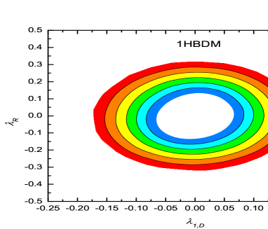
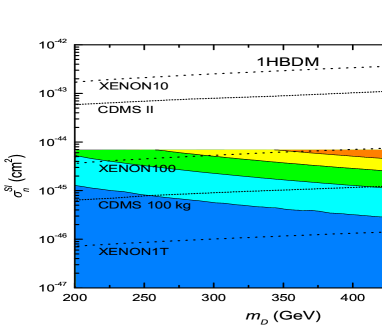
Figure 2: Left panels: the predicted coupling $\lambda_{1,D}$ as a function of $\lambda_{R}$ and the DM mass $m_{D}$ from the observed DM abundance in the 1HBDM. Right panels: the predicted DM-nucleon scattering cross section $\sigma_{n}^{SI}$ in the 1HBDM with current and future experimental upper bounds.

In terms of the observed DM abundance $0.1088\leq\Omega_{D}h^{2}\leq 0.1158$ WMAP7 , we numerically solve the Boltzmann equation and derive the coupling $\lambda_{1,D}$ with different $\lambda_{R}$ for $10\,{\rm GeV}\leq m_{D}\leq 200\,{\rm GeV}$. The numerical results are shown in Fig. 2 (upper-left panel). Due to the resonance contribution, a very small value of the coupling $\lambda_{1,D}$ can be derived from the observed DM abundance for the resonance region ($0.8\;m_{h^{0}}\lesssim 2m_{D}<m_{h^{0}}$). Except for the resonance region, one may find $\lambda_{1,D}\sim{\cal O}(10^{-2}-10^{-1})$. The parameter $\lambda_{R}$ plays an important role to determine the DM relic density if $m_{D}>m_{h^{0}}$. For illustration, we also plot the $\lambda_{R}=\pm 0.1$ cases which can significantly change the predicted $\lambda_{1,D}$ as shown in Fig. 2. In fact, $\lambda_{1,D}$ may be very small (even to be zero) for the larger $|\lambda_{R}|$. In this case, the $H_{2}^{0}$-exchange annihilation process is dominant. Here we have assumed $\lambda_{1,D}$ is positive. If we simultaneously change the signs of $\lambda_{1,D}$ and $\lambda_{R}$, the negative $\lambda_{1,D}$ case may be approximately induced from the positive case. This feature can be well understood from Eqs. (10-11). It should be mentioned that the thermally averaged annihilation cross section $\langle\sigma v\rangle$ will significantly change as the evolution of the Universe when the DM particle is nearly one-half the mass of a resonance BW . This is the Breit-Wigner resonance effect which has been used to explain the recent PAMELA PAMELA , ATIC ATIC and Fermi Fermi anomalies. Notice that the decaying $S_{D}$ with a lifetime around ${\cal O}(10^{26}s)$ can also account for the electron and positron anomalies Guo:2010vy . Here we have considered the Breit-Wigner resonance effect for the determination of the coupling $\lambda_{1,D}$.

For $200\,{\rm GeV}\leq m_{D}\leq 500\,{\rm GeV}$, we use the approximate formulas to scan the whole parameter space $\lambda_{1,D}$ and $\lambda_{R}$. The allowed parameter space is shown in Fig. 2 (lower-left panel), which gives an allowed range $-0.17\lesssim\lambda_{1,D}\lesssim 0.17$ and $-0.32\lesssim\lambda_{R}\lesssim 0.32.$ The central region of this figure is excluded since these points can not provide large enough annihilation cross section to give the desired DM abundance. Notice that the approximate global symmetry $U(1)$ requires $m_{D}^{2}/v_{R}^{2}\ll\lambda_{1,D}$ which means the region near $\lambda_{1,D}=0$ is disfavored.

III.2 Dark matter direct search

For the scalar dark matter, the DM elastic scattering cross section on a nucleon is spin-independent, which is given by DM

$$\sigma_{n}^{SI}\approx\frac{4}{\pi}\left(\frac{m_{D}\;m_{n}}{m_{D}+m_{n}}\right)^{2}\frac{(Zf_{p}+(A-Z)f_{n})^{2}}{A^{2}}\;,$$ (20)

where $m_{n}$ is the nucleon mass. $Z$ and $A-Z$ are the numbers of protons and neutrons in the nucleus. $f_{p,n}$ is the coupling between DM and protons or neutrons, given by

$$f_{p,n}=\sum_{q=u,d,s}f_{Tq}^{(p,n)}a_{q}\frac{m_{p,n}}{m_{q}}+\frac{2}{27}f_{TG}^{(p,n)}\sum_{q=c,b,t}a_{q}\frac{m_{p,n}}{m_{q}},$$ (21)

where $f_{Tu}^{(p)}=0.020\pm 0.004$, $f_{Td}^{(p)}=0.026\pm 0.005$, $f_{Ts}^{(p)}=0.118\pm 0.062$, $f_{Tu}^{(n)}=0.014\pm 0.003$, $f_{Td}^{(n)}=0.036\pm 0.008$ and $f_{Ts}^{(n)}=0.118\pm 0.062$ Ellis:2000ds . The coupling $f_{TG}^{(p,n)}$ between DM and gluons from heavy quark loops is obtained from $f_{TG}^{(p,n)}=1-\sum_{q=u,d,s}f_{Tq}^{(p,n)}$, which leads to $f_{TG}^{(p)}\approx 0.84$ and $f_{TG}^{(n)}\approx 0.83$. In our model, the DM-quark coupling $a_{q}$ in Eq. (21) is given by

$$a_{q}=\frac{\lambda_{1,D}\;m_{q}}{2m_{D}\;m_{h^{0}}^{2}}\,.$$ (22)

Because of $f_{n}\approx f_{p}$, we can derive

$$\sigma_{n}^{SI}\approx\frac{4}{\pi}\left(\frac{m_{D}\;m_{n}}{m_{D}+m_{n}}\right)^{2}f_{n}^{2}\;.$$ (23)

It is worthwhile to stress that $\sigma_{n}^{SI}$ is independent of $\lambda_{R}$.

Using the predicted $\lambda_{1,D}$ from the observed DM abundance, we straightly calculate the spin-independent DM-nucleon elastic scattering cross section $\sigma_{n}^{SI}$. The numerical results are shown in Fig. 2 (right panels). For $10\,{\rm GeV}\leq m_{D}\leq 200\,{\rm GeV}$, we find that two DM mass ranges can be excluded by the current DM direct detection experiments CDMS II CDMSII and XENON10 XENON10 . Due to the existence of $\lambda_{R}$, we can obtain different values of $\sigma_{n}^{SI}$ for a given DM mass $m_{D}$ when the annihilation channel $S_{D}S_{D}\rightarrow h^{0}h^{0}$ is open. In this case, one can obtain $\sigma_{n}^{SI}\lesssim 7\times 10^{-45}{\rm cm}^{2}$ for $200\,{\rm GeV}\leq m_{D}\leq 500\,{\rm GeV}$ as shown in Fig. 2 (lower-right panel), which is below the current experimental upper bounds. Nevertheless the future experiments XENON100 XENON100P , CDMS 100 kg CDMS100 and XENON1T XENON1T can cover most parts of the allowed parameter space. For the region near the resonance point, the predicted $\sigma_{n}^{SI}$ is far below the current and future experimental upper bounds.

III.3 Dark matter indirect search

As shown in Sec. III.1, $\langle\sigma v\rangle$ is a key quantity in the determination of the DM cosmic relic abundance. On the other hand, $\langle\sigma v\rangle$ also determines the DM annihilation rate in the galactic halo. It should be mentioned that the DM annihilation in the galactic halo occurs at $v\approx 10^{-3}$ ($x\approx 3/v^{2}=3\times 10^{6}$). Thus we calculate the thermally averaged annihilation cross section at $x\approx 3\times 10^{6}$, namely $\langle\sigma v\rangle_{0}$. The numerical results have been shown in Fig. 3 for $10\,{\rm GeV}\leq m_{D}\leq 200\,{\rm GeV}$. Notice that we can derive the similar results for different values of $\lambda_{R}$. One may find $1\times 10^{-26}\;{\rm cm}^{3}\;{\rm sec}^{-1}\leq\langle\sigma v\rangle_{0}\leq 3\times 10^{-26}\;{\rm cm}^{3}\;{\rm sec}^{-1}$ for most parts of the parameter space. The enhanced and suppressed $\langle\sigma v\rangle_{0}$ on the two sides of the resonance point originate from the Breit-Wigner resonance effect BW . When $m_{D}$ is slightly less than the $W_{1}$ boson mass, the channel $S_{D}S_{D}\rightarrow W_{1}^{+}W_{1}^{-}$ is open at high temperature, which dominates the total thermally averaged annihilation cross section and determines the DM relic density. However this channel is forbidden in the galactic halo. Thus the threshold effect leads to a dip around $W_{1}$ threshold Threshold . When $200\,{\rm GeV}\leq m_{D}\leq 500\,{\rm GeV}$, one can obtain $\langle\sigma v\rangle_{0}\approx 2.3\times 10^{-26}\;{\rm cm}^{3}\;{\rm sec}^{-1}$ which is consistent with the usual $s$-wave annihilation cross section $\langle\sigma v\rangle\approx 3\times 10^{-26}\;{\rm cm}^{3}\;{\rm sec}^{-1}$ at the freeze-out temperature $x_{f}\approx 20$.

Figure 3: The predicted thermally averaged DM annihilation cross section $\langle\sigma v\rangle_{0}$ in the 1HBDM.

In our model, the DM annihilation can generate primary antiprotons which can be detected by the DM indirect search experiments. Recently, the PAMELA collaboration reports that the observed antiproton data is consistent with the usual estimation value of the secondary antiproton PAMELA . Therefore one can use the PAMELA antiproton measurements to constrain $\langle\sigma v\rangle_{0}$. In Fig. 3, we have also shown the maximum allowed $\langle\sigma v\rangle_{0}$ for the MIN, MED and MAX antiproton propagation models given in Ref. Goudelis:2009zz . Then we can find that a very narrow region can be excluded by the PAMELA antiproton data in our model. In fact, the width of this excluded region is about $0.4$ GeV for the MED and MAX cases. When double DM mass $2m_{D}$ is slightly less than the Higgs mass $m_{h^{0}}$, the predicted $\sigma_{n}^{SI}$ and $\langle\sigma v\rangle_{0}$ are very small which means that it is very difficult to detect the DM signals.

IV Dark matter signal in the 2HBDM

We have discussed the Higgs singlet $S_{D}$ as the cold DM candidate in the 1HBDM. In this section, we generalize the previous discussions to the 2HBDM in which the other bidoublet $\chi$ mixes significantly with $\phi$ and $\Delta_{L,R}$. In this case the SCPV can be easily realized Wu:2007kt . Comparing with the previous case, the main differences are that there could be more scalar particles entering the DM annihilation and scattering processes. Furthermore, the new contributions from these particles may modify the correlation between the DM annihilation and DM-nucleon elastic scattering cross sections, which leads to significantly different predictions from the other singlet scalar DM models and the previous discussions.

As shown in Eq. (1), the second Higgs bidoublet $\chi$ contains two neutral Higgs contents $\chi_{1,2}^{0}$. After the SSB, $\chi_{1,2}^{0}$ may obtain the VEVs $w_{1,2}/\sqrt{2}$. The squared sum of all the VEVs including $\kappa_{1,2}$ should still lead to $v_{\rm EW}=\sqrt{|\kappa_{1}|^{2}+|\kappa_{1}|^{2}+|w_{1}|^{2}+|w_{2}|^{2}}\approx 246$ GeV. In general, the 2HBDM includes three light neutral Higgs bosons and a pair of charged light Higgs particles, whose masses are order of the electroweak energy scale. For simplicity, we consider $\kappa_{2}\sim w_{2}\sim 0$. In this case, it is convenient for us to rotate Higgs bidoublets $\phi$ and $\chi$ into

$$\phi^{\prime}=\left(\begin{matrix}\frac{h_{1}+v_{\rm EW}}{\sqrt{2}}&{\phi^{\prime}}_{2}^{+}\cr 0&{\phi^{\prime}}_{2}^{0}\cr\end{matrix}\right),\;\chi^{\prime}=\left(\begin{matrix}\frac{h_{2}+ih_{3}}{\sqrt{2}}&{\chi^{\prime}}_{2}^{+}\cr H^{-}&{\chi^{\prime}}_{2}^{0}\cr\end{matrix}\right)\;,$$ (24)

where $H^{\pm}$ are a pair of light charged Higgs bosons. Then one can diagonalize the mass matrix of three light neutral Higgs $h_{1,2,3}$ and derive three light neutral Higgs mass eigenstates. The relation between $h_{1,2,3}$ and three mass eigenstates can be written as

$$\left(\begin{matrix}h_{1}\cr h_{2}\cr h_{3}\cr\end{matrix}\right)\;=\;\left(\begin{matrix}c^{~{}}_{x}c^{~{}}_{z}&s^{~{}}_{x}c^{~{}}_{z}&s^{~{}}_{z}\cr-c^{~{}}_{x}s^{~{}}_{y}s^{~{}}_{z}-s^{~{}}_{x}c^{~{}}_{y}&-s^{~{}}_{x}s^{~{}}_{y}s^{~{}}_{z}+c^{~{}}_{x}c^{~{}}_{y}&s^{~{}}_{y}c^{~{}}_{z}\cr-c^{~{}}_{x}c^{~{}}_{y}s^{~{}}_{z}+s^{~{}}_{x}s^{~{}}_{y}&-s^{~{}}_{x}c^{~{}}_{y}s^{~{}}_{z}-c^{~{}}_{x}s^{~{}}_{y}&c^{~{}}_{y}c^{~{}}_{z}\cr\end{matrix}\right)\;\left(\begin{matrix}h\cr H\cr A\cr\end{matrix}\right)\;,$$ (25)

where $s_{x}\equiv\sin\theta_{x}$, $c_{x}\equiv\cos\theta_{x}$ and so on. Due to many unknown parameters in the Higgs potential of 2HBDM, we can not explicitly calculate three mixing angles $\theta_{x},\theta_{y}$ and $\theta_{z}$. For illustration, we consider three representative cases: (I) $\theta^{~{}}_{x}=60^{\circ}$, $\theta^{~{}}_{y}=60^{\circ}$ and $\theta^{~{}}_{z}=150^{\circ}$; (II) $\theta^{~{}}_{x}=30^{\circ}$, $\theta^{~{}}_{y}=0^{\circ}$ and $\theta^{~{}}_{z}=0^{\circ}$; (III) $\theta^{~{}}_{x}=0^{\circ}$, $\theta^{~{}}_{y}=90^{\circ}$ and $\theta^{~{}}_{z}=75^{\circ}$. The Case I means that there is the significant mixing among three light neutral Higgs. If all $CP$ violation phases are absent, we can obtain $\theta^{~{}}_{y}=0^{\circ}$ and $\theta^{~{}}_{z}=0^{\circ}$. In the Case II, the light Higgs $A$ is $CP$ odd which does not mix with $h$ and $H$. For the Case III, we only consider the scalar and pseudoscalar mixing, namely $\theta^{~{}}_{x}=0^{\circ}$.

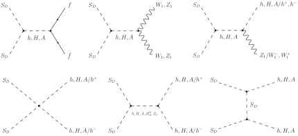
Figure 4: Feynman diagrams for the DM annihilation in the 2HBDM.

In the 2HBDM, the possible DM annihilation products are $f\bar{f}$, $W_{1}W_{1}/Z_{1}Z_{1}$, $W_{1}^{\pm}H^{\mp}/Z_{1}(h,H,A)$, $H^{+}H^{-}$ and any two of the three neutral states $(h,H,A)$ as shown in Fig. 4. For a concrete numerical illustration, we choose all the masses $m_{H}$, $m_{A}$, $m_{H^{\pm}}=180$ GeV and $m_{h}=120$ GeV. For cubic and quartic scalar vertexes, we assume they are the same as that in the 1HBDM. Namely, the vertexes of $S_{D}S_{D}(h,H,A)$ and $S_{D}S_{D}(h,H,A/H^{+})(h,H,A/H^{-})$ are set equal to $-i\lambda_{1,D}v_{\rm EW}$ and $-i\lambda_{1,D}$, respectively. Similarly, the cubic scalar vertexes among the light Higgs particles $h$, $H,A$ and $H^{\pm}$ are set equal to $-i3m_{h}^{2}/v_{\rm EW}$, and the cubic scalar vertexes between $S_{\sigma}$ and two light Higgs particles are assumed to be $-i\lambda_{1,D}v_{\sigma}$. It is worthwhile to stress that the heavy Higgs particles from $\chi^{\prime}$ may be as the intermediate particles when two DM candidates annihilate into two light Higgs bosons. Nevertheless we still can use a coupling $\lambda_{R}$ to describe the contributions of all possible heavy Higgs bosons. All annihilation cross sections $\hat{\sigma}$ have been presented in Appendix A.

In the basis of Eq. (24), the Yukawa interactions for quarks are given by

$$-{\cal L}_{Y}=\overline{Q_{L}}\left(Y^{\phi}\phi^{\prime}+\tilde{Y}^{\phi}\tilde{\phi^{\prime}}+Y^{\chi}\chi^{\prime}+\tilde{Y}^{\chi}\tilde{\chi^{\prime}}\right)Q_{R}+h.c.,$$ (26)

where $Q_{L,R}=(u_{L,R},d_{L,R})^{T}$. When both $P$ and $CP$ are required to be broken down spontaneously, the Yukawa coupling matrices $Y^{\phi}$, $\tilde{Y}^{\phi}$, $Y^{\chi}$ and $\tilde{Y}^{\chi}$ are complex symmetric. Then one may rotate the quark fields and derive the following Yukawa interactions relevant to light neutral Higgs particles:

$$-{\cal L}_{LH}=\frac{h_{1}+v_{\rm EW}}{\sqrt{2}}\left(\overline{u^{\prime}_{L}}Y^{\phi^{\prime}}u^{\prime}_{R}+\overline{d^{\prime}_{L}}\tilde{Y}^{\phi^{\prime}}d^{\prime}_{R}\right)+\frac{h_{2}+ih_{3}}{\sqrt{2}}\overline{u^{\prime}_{L}}Y^{\chi^{\prime}}u^{\prime}_{R}+\frac{h_{2}-ih_{3}}{\sqrt{2}}\overline{d^{\prime}_{L}}\tilde{Y}^{\chi^{\prime}}d^{\prime}_{R}+h.c.,$$ (27)

where $Y^{\phi^{\prime}}$ and $\tilde{Y}^{\phi^{\prime}}$ are diagonal matrixes. According to the up and down quark masses, we can obtain $Y^{\phi^{\prime}}_{qq}=\sqrt{2}m_{q}/v_{\rm EW}$ and $\tilde{Y}^{\phi^{\prime}}_{qq}=\sqrt{2}m_{q}/v_{\rm EW}$, respectively. In order to avoid the FCNC processes, we assume $Y^{\chi^{\prime}}$ and $\tilde{Y}^{\chi^{\prime}}$ are approximate diagonal matrixes due to approximate $U(1)$ family symmetries Wu and require

$$Y^{\chi^{\prime}}_{qq}=R_{q}\,Y^{\phi^{\prime}}_{qq}\;{\rm and}\;\tilde{Y}^{\chi^{\prime}}_{qq}=R_{q}\,\tilde{Y}^{\phi^{\prime}}_{qq}\;.$$ (28)

Since $Y^{\chi^{\prime}}$ and $\tilde{Y}^{\chi^{\prime}}$ don’t contribute the quark masses, the parameter $R_{q}$ may be very large except the top quark case.

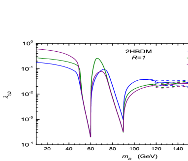
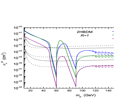
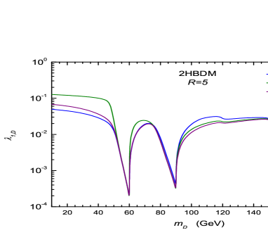
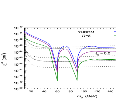
Figure 5: The predicted coupling $\lambda_{1,D}$ and DM-nucleon scattering cross section $\sigma_{n}^{SI}$ for three mixing cases in the 2HBDM with $R=1$ and $R=5$.

In the 2HBDM, the parameter $R_{q}$ in Eq. (28) controls the Yukawa couplings $Y^{\chi^{\prime}}_{qq}$ and $\tilde{Y}^{\chi^{\prime}}_{qq}$. Furthermore, the parameter $R_{q}$ will affect the total annihilation cross section and change the predicted coupling $\lambda_{1,D}$. For illustration, we choose the following two scenarios

$$R_{q}\equiv R=1\;{\rm and}\;R_{q}\equiv R=5\;(q\neq t\;{\rm and}\;R_{t}=1\;{\rm for\;the\;top\;quark})$$ (29)

to calculate the allowed coupling $\lambda_{1,D}$ from the observed DM abundance. Considering three kinds of mixing cases and two $R$ scenarios, we plot the allowed coupling $\lambda_{1,D}$ for $10\,{\rm GeV}\leq m_{D}\leq 200\,{\rm GeV}$ in Fig. 5 (left panels). It is clear that $\lambda_{1,D}$ is dependent on the light Higgs mixing and the parameter $R$ if $m_{D}<120$ GeV. When DM candidate can annihilate into two light Higgs bosons ($m_{D}\gtrsim 120$ GeV), one can derive the almost same $\lambda_{1,D}$ for three kinds of mixing cases and two $R$ scenarios, which means that the light Higgs mixing and the parameter $R$ do not significantly affect the total annihilation cross section. This conclusion can also be applied to $200\,{\rm GeV}\leq m_{D}\leq 500\,{\rm GeV}$ as shown in Figs. 7 and 8 (left panels).

For the DM indirect search, the 2HBDM has two enhanced regions for $\langle\sigma v\rangle_{0}$ as shown in Fig. 6. Therefore the PAMELA antiproton measurements can exclude two very narrow regions. The predicted $\langle\sigma v\rangle_{0}$ is the same as that in the 1HBDM for most parts of parameter space. When $200\,{\rm GeV}\leq m_{D}\leq 500\,{\rm GeV}$, one can still obtain $\langle\sigma v\rangle_{0}\approx 2.3\times 10^{-26}\;{\rm cm}^{3}\;{\rm sec}^{-1}$. It is clear that different mixing cases and $R$ scenarios lead to the same $\langle\sigma v\rangle_{0}$ except the resonance regions.

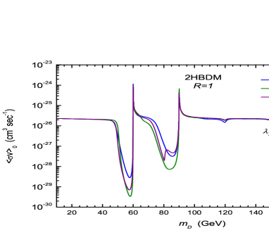
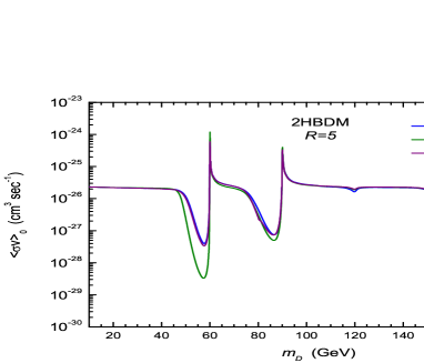
Figure 6: The predicted thermally averaged DM annihilation cross section $\langle\sigma v\rangle_{0}$ in the 2HBDM.

In the 2HBDM, the DM-quark coupling $a_{q}$ in Eq. (21) is given by

$$a_{q}=\frac{\lambda_{1,D}\,m_{q}}{2m_{D}}\left(\frac{f_{1}}{m^{2}_{h}}+\frac{f_{3}}{m^{2}_{H}}+\frac{f_{5}}{m^{2}_{A}}\right)\,,$$ (30)

where $f_{i}$ have been presented in Appendix Eq. (33). Notice that we have neglected the parameters $f_{2}$, $f_{4}$ and $f_{6}$ since their contributions to $\sigma_{n}^{SI}$ are velocity-dependent. Using the predicted $\lambda_{1,D}$ in Fig. 5 (left panels), we calculate the spin-independent DM-nucleon elastic scattering cross section $\sigma_{n}^{SI}$ for three mixing cases and two $R$ scenarios. Different from $\langle\sigma v\rangle_{0}$, the predicted $\sigma_{n}^{SI}$ obviously depends on the mixing and $R$ as shown in Fig. 5 (right panels). Although three kinds of mixing cases have the almost same coupling $\lambda_{1,D}$ for $m_{D}\gtrsim 120$ GeV in the $R=1$ scenario, the predicted $\sigma_{n}^{SI}$ in the Case III is far less than that in the Case I and Case II. This is because that there is cancellation between $f_{1}/m_{h}^{2}$ and $f_{5}/m_{A}^{2}$ in Eq. (30) for the Case III. When the DM candidate can annihilate into two light Higgs bosons, a large $R$ does not obviously affect the predicted coupling $\lambda_{1,D}$. However, the parameters $f_{1},f_{3}$ and $f_{5}$ in Eq. (30) will be significantly enlarged. Therefore $\sigma_{n}^{SI}$ usually increases as $R$ increases. The Case I clearly demonstrates this feature. The enlarged $\sigma_{n}^{SI}$ in the $R=5$ scenario may approach the CDMS II upper bound, which can be used to explain the two possible events observed by the CDMS II CDMSII . It is worthwhile to stress that the Case II in the $R=5$ scenario give a smaller $\sigma_{n}^{SI}$ than that in the $R=1$ scenario due to the cancellation from the different Higgs boson contributions. We conclude that the predicted $\sigma_{n}^{SI}$ is significantly dependent on the light Higgs mixing and the parameter $R$. For $200\,{\rm GeV}\leq m_{D}\leq 500\,{\rm GeV}$, the same conclusion can also be derived as shown in Figs. 7 and 8 (right panels).

As shown in Figs. 5, 7 and 8 (right panels), the CDMS II CDMSII and XENON10 XENON10 experiments can exclude the region $m_{D}\lesssim 50$ GeV. For $200\,{\rm GeV}\leq m_{D}\leq 500$ GeV, our results show an upper bound for $\sigma_{n}^{SI}$ which is still below the current experiment upper bounds. The future experiments XENON100 XENON100P , CDMS 100 kg CDMS100 and XENON1T XENON1T can cover most parts of the allowed parameter space except the extreme cancellation cases. Nevertheless, it is still difficult to detect the DM direct or indirect signals for the resonance regions $50\,{\rm GeV}\lesssim m_{D}\lesssim 60$ GeV and $80\,{\rm GeV}\lesssim m_{D}\lesssim 90$ GeV.

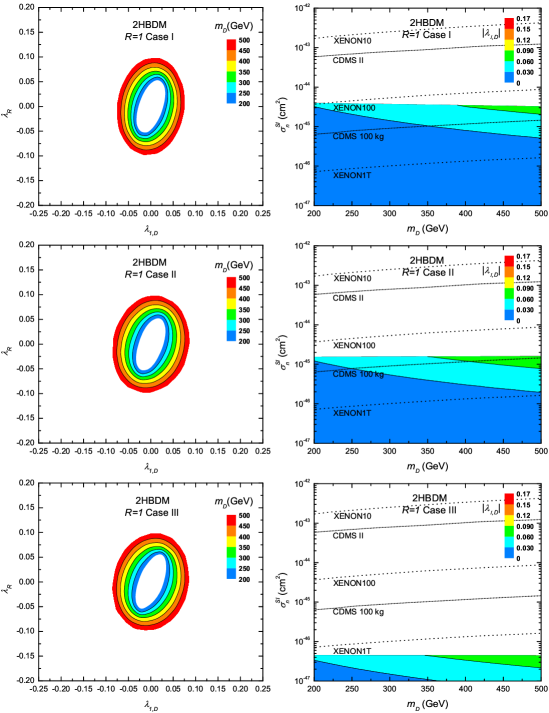
Figure 7: The allowed parameter space and the predicted $\sigma_{n}^{SI}$ for three mixing cases in the 2HBDM with $R=1$.

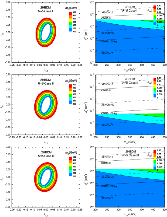
Figure 8: The allowed parameter space and the predicted $\sigma_{n}^{SI}$ for three mixing cases in the 2HBDM with $R=5$.

V Conclusions

In conclusion, we have investigated a scalar boson $S_{D}$ as the DM candidate in the left-right symmetric gauge model with two Higgs bidoublets, in which the SCPV can be easily realized. The stability of DM candidate $S_{D}$ is ensured by the fundamental symmetries $P$ and $CP$ of quantum field theory. In order to well understand the DM properties in the 2HBDM, we have firstly analyzed the 1HBDM and shown that the predicted DM direct and indirect detection cross sections ($\sigma_{n}^{SI}$ and $\langle\sigma v\rangle_{0}$) are the same as that in the minimal extension of SM with a real singlet scalar if $m_{D}<m_{h^{0}}$. When the annihilation channel $S_{D}S_{D}\rightarrow h^{0}h^{0}$ is open ($m_{D}>m_{h^{0}}$), the $H_{2}^{0}$ exchange diagram relevant to $\lambda_{R}$ leads to a continuous DM-nucleon elastic scattering cross sections $\sigma_{n}^{SI}$. Comparing with the 1HBDM, there are more scalar particles entering the DM annihilation and scattering processes in the 2HBDM. In the explicit calculations, we have considered three typical mixing cases and two Yukawa coupling scenarios ($R=1$ and $R=5$) to analyze the 2HBDM. It has been shown that $\langle\sigma v\rangle_{0}$ is not sensitive to the light Higgs mixing and Yukawa couplings except the resonance regions. However $\sigma_{n}^{SI}$ is significantly dependent on the above two factors. In general, $\sigma_{n}^{SI}$ can be enhanced by large Yukawa couplings and approach the CDMS II upper bound, which can be used to explain the two possible events observed by CDMS II. It should be mentioned that a large Yukawa coupling may lead to a very small $\sigma_{n}^{SI}$ in the extreme mixing case. Our results show that the future DM direct search experiments can cover most parts of the allowed parameter space. The PAMELA antiproton data can exclude two very narrow regions in the 2HBDM. In addition, we have shown that it is very difficult to detect the DM direct or indirect signals for the resonance regions since the Breit-Wigner resonance effect simultaneously suppresses $\sigma_{n}^{SI}$ and $\langle\sigma v\rangle_{0}$.

Appendix A Annihilation cross section

For the annihilation processes $S_{D}\,S_{D}\rightarrow f{\bar{f}}$, the annihilation cross section $\hat{\sigma}_{f\bar{f}}$ is given by

$$\hat{\sigma}_{f\bar{f}}=\sum_{f}m_{f}^{2}\frac{\lambda_{1,D}^{2}}{4\pi}\sqrt{1-\frac{4m_{f}^{2}}{s}}\left[(s-4m_{f}^{2})P_{1}+sP_{2}\right],$$ (31)

where

$$P_{1,2}=\left|\frac{f_{1,2}}{s-m_{h}^{2}+im_{h}\Gamma_{h}}+\frac{f_{3,4}}{s-m_{H}^{2}+im_{H}\Gamma_{H}}+\frac{f_{5,6}}{s-m_{A}^{2}+im_{A}\Gamma_{A}}\right|^{2}\;,$$ (32)

with

$$f_{1}=c_{x}c_{z}-Rc_{y}s_{x}-Rc_{x}s_{y}s_{z}\;, f_{2}=Rs_{x}s_{y}-Rc_{x}c_{y}s_{z}\;,$$ (33)

$$f_{3}=Rc_{x}c_{y}+c_{z}s_{x}-Rs_{x}s_{y}s_{z}\;, f_{4}=-Rs_{x}s_{z}c_{y}-Rc_{x}s_{y}\;,$$

$$f_{5}=Rs_{y}c_{z}+s_{z}\;,\;\;\;\;\;\;\;\;\;\;\;\;\;\;\;\;\;\; f_{6}=Rc_{y}c_{z}\;.$$

The parameter $R$ has been defined in Eq. (29). The decay widths of three light neutral Higgs are given by

$$\Gamma_{h,H,A}=\frac{\sum m_{f}^{2}}{8\pi v_{\rm EW}^{2}}m_{h,H,A}(f_{1,3,5}^{2}+f_{2,4,6}^{2})+\Gamma_{h,H,A}^{Z_{1}}\gamma_{h,H,A}+\Gamma_{h,H,A}^{W_{1}}\gamma_{h,H,A}+\frac{\lambda_{1,D}^{2}v_{\rm EW}^{2}}{32\pi}\frac{\sqrt{m_{h,H,A}^{2}-4m_{D}^{2}}}{m_{h,H,A}^{2}}\;,$$ (34)

where $\gamma_{h}=c_{x}^{2}c_{z}^{2}$, $\gamma_{H}=s_{x}^{2}c_{z}^{2}$ and $\gamma_{A}=s_{z}^{2}$. $\Gamma_{h,H,A}^{Z_{1}}$ and $\Gamma_{h,H,A}^{W_{1}}$ have the following forms:

$$\Gamma_{h,H,A}^{Z_{1}} = \frac{m_{h,H,A}^{3}}{32\pi v_{\rm EW}^{2}}\sqrt{1-\frac{4m_{Z_{1}}^{2}}{m_{h,H,A}^{2}}}\left(1-\frac{4m_{Z_{1}}^{2}}{m_{h,H,A}^{2}}+\frac{12m_{Z_{1}}^{4}}{m_{h,H,A}^{4}}\right)\;,$$ (35)

$$\Gamma_{h,H,A}^{W_{1}} = \frac{m_{h,H,A}^{3}}{16\pi v_{\rm EW}^{2}}\sqrt{1-\frac{4m_{W_{1}}^{2}}{m_{h,H,A}^{2}}}\left(1-\frac{4m_{W_{1}}^{2}}{m_{h,H,A}^{2}}+\frac{12m_{W_{1}}^{4}}{m_{h,H,A}^{4}}\right)\;.$$

For the annihilation processes $S_{D}\,S_{D}\rightarrow Z_{1}Z_{1}$ and $S_{D}\,S_{D}\rightarrow W_{1}W_{1}$, we have

$$\hat{\sigma}_{Z_{1}Z_{1}} = \frac{\lambda_{1,D}^{2}}{16\pi}\sqrt{1-\frac{4m_{Z_{1}}^{2}}{s}}\left(1-\frac{4m_{Z_{1}}^{2}}{s}+\frac{12m_{Z_{1}}^{4}}{s^{2}}\right)\frac{s^{2}}{4}$$ (36)

$$\times \left|\frac{2c_{x}c_{z}}{s-m_{h}^{2}+im_{h}\Gamma_{h}}+\frac{2s_{x}c_{z}}{s-m_{H}^{2}+im_{H}\Gamma_{H}}+\frac{2s_{z}}{s-m_{A}^{2}+im_{A}\Gamma_{A}}\right|^{2},$$

$$\hat{\sigma}_{W_{1}W_{1}} = \frac{\lambda_{1,D}^{2}}{8\pi}\sqrt{1-\frac{4m_{W_{1}}^{2}}{s}}\left(1-\frac{4m_{W_{1}}^{2}}{s}+\frac{12m_{W_{1}}^{4}}{s^{2}}\right)\frac{s^{2}}{4}$$ (37)

$$\times \left|\frac{2c_{x}c_{z}}{s-m_{h}^{2}+im_{h}\Gamma_{h}}+\frac{2s_{x}c_{z}}{s-m_{H}^{2}+im_{H}\Gamma_{H}}+\frac{2s_{z}}{s-m_{A}^{2}+im_{A}\Gamma_{A}}\right|^{2}.$$

If the annihilation productions are a Higgs and a gauge boson, we can derive

$$\hat{\sigma}_{Z_{1}A} = \frac{\lambda_{1,D}^{2}}{32\pi}\frac{\left[(s-m_{A}^{2}-m_{Z_{1}}^{2})^{2}-4m_{A}^{2}m_{Z_{1}}^{2}\right]^{1.5}}{s}\left|\frac{2c_{z}s_{x}}{s-m_{h}^{2}}-\frac{2c_{x}c_{z}}{s-m_{H}^{2}}\right|^{2}\;,$$

$$\hat{\sigma}_{Z_{1}H} = \frac{\lambda_{1,D}^{2}}{32\pi}\frac{\left[(s-m_{H}^{2}-m_{Z_{1}}^{2})^{2}-4m_{H}^{2}m_{Z_{1}}^{2}\right]^{1.5}}{s}\left|\frac{2c_{x}c_{z}}{s-m_{A}^{2}}-\frac{2s_{z}}{s-m_{h}^{2}}\right|^{2}\;,$$

$$\hat{\sigma}_{Z_{1}h} = \frac{\lambda_{1,D}^{2}}{32\pi}\frac{\left[(s-m_{h}^{2}-m_{Z_{1}}^{2})^{2}-4m_{h}^{2}m_{Z_{1}}^{2}\right]^{1.5}}{s}\left|\frac{2s_{z}}{s-m_{H}^{2}}-\frac{2c_{z}s_{x}}{s-m_{A}^{2}}\right|^{2}\;,$$

$$\hat{\sigma}_{W^{\pm}H^{\mp}} = \frac{\lambda_{1,D}^{2}}{4\pi}\frac{\left[(s-m_{H^{\pm}}^{2}-m_{W_{1}}^{2})^{2}-4m_{H^{\pm}}^{2}m_{W_{1}}^{2}\right]^{1.5}}{s}\left|\frac{a_{1}}{s-m_{A}^{2}}+\frac{a_{2}}{s-m_{H}^{2}}+\frac{a_{3}}{s-m_{h}^{2}}\right|^{2},$$ (38)

where

$$a_{1} = c_{y}c_{z}-ic_{z}s_{y}\;,$$

$$a_{2} = -c_{x}(ic_{y}+s_{y})-c_{y}s_{x}s_{z}+is_{x}s_{y}s_{z}\;,$$

$$a_{3} = ic_{y}s_{x}+s_{y}s_{x}-c_{x}(c_{y}s_{z}-is_{y}s_{z})\;.$$ (39)

When two DM candidates annihilate into two Higgs particles, we can obtain

$$\hat{\sigma}_{kk} = \frac{\lambda_{1,D}^{2}}{16\pi}\sqrt{1-\frac{4m_{k}^{2}}{s}}\left[G_{2}^{2}-\frac{8\lambda_{1,D}v_{\rm EW}^{2}}{s-2m_{k}^{2}}G_{2}F({\xi_{kk}})+\frac{8\lambda_{1,D}^{2}v_{\rm EW}^{4}}{(s-2m_{k}^{2})^{2}}\left(\frac{1}{1-\xi_{kk}^{2}}+F({\xi_{kk}})\right)\right]\;,$$

$$\hat{\sigma}_{ij} = \frac{\lambda_{1,D}^{2}}{8\pi}\beta_{ij}\left[G_{2}^{2}-\frac{8\lambda_{1,D}v_{\rm EW}^{2}}{s-m_{i}^{2}-m_{j}^{2}}G_{2}F({\xi_{ij}})+\frac{8\lambda_{1,D}^{2}v_{\rm EW}^{4}}{(s-m_{i}^{2}-m_{j}^{2})^{2}}\left(\frac{1}{1-\xi_{ij}^{2}}+F({\xi_{ij}})\right)\right],$$

$$\hat{\sigma}_{H^{\pm}H^{\mp}} = \frac{\lambda_{1,D}^{2}}{8\pi}\sqrt{1-\frac{4m_{H^{\pm}}^{2}}{s}}G_{2}^{2},$$ (40)

with

$$G_{2} = 1+\frac{3m_{h}^{2}}{s-m_{h}^{2}}+\frac{3m_{h}^{2}}{s-m_{H}^{2}}+\frac{3m_{h}^{2}}{s-m_{A}^{2}}+\frac{\alpha_{1}\lambda_{3,D}v_{R}^{2}}{s-m_{H_{2}^{0}}^{2}}\frac{1}{\lambda_{1,D}}+\frac{m_{\sigma}^{2}}{s-m_{\sigma}^{2}}.$$ (41)

The subscripts $k$ and $ij$ run over ($h,H,A$) and ($hH,hA,HA$), respectively. The quantity $F$ is defined as $F(\xi)\equiv\mbox{arctanh}(\xi)/\xi$ with $\xi_{ij}=\sqrt{1-4m_{D}^{2}/s}\sqrt{(s-m_{i}^{2}-m_{j}^{2})^{2}-4m_{i}^{2}m_{j}^{2}}/(s-m_{i}^{2}-m_{j}^{2})$. The parameter $\beta_{ij}$ is given by $\beta_{ij}=\sqrt{(s-m_{i}^{2}-m_{j}^{2})^{2}-4m_{i}^{2}m_{j}^{2}}/{s}$.

References

(1) For reviews, see, e.g., G. Jungman, M. Kamionkowski and K.
Griest, Phys. Rept. 267, 195 (1996); G. Bertone, D. Hooper and
J. Silk, Phys. Rept. 405, 279 (2005).
(2)
E. Komatsu et al.,
arXiv:1001.4538 [astro-ph.CO].
(3)
J. C. Pati and A. Salam,
Phys. Rev. D 10, 275 (1974)
[Erratum-ibid. D 11, 703 (1975)];
R. N. Mohapatra and J. C. Pati,
Phys. Rev. D 11, 566 (1975);
G. Senjanovic and R. N. Mohapatra,
Phys. Rev. D 12, 1502 (1975);
R. N. Mohapatra and G. Senjanovic, Phys. Rev. Lett. 44, 912
(1980); Phys. Rev. D 23, 165 (1981).
(4)
G. Beall, M. Bander and A. Soni,
Phys. Rev. Lett. 48, 848 (1982).
(5)
N. G. Deshpande, J. F. Gunion, B. Kayser and F. I. Olness,
Phys. Rev. D 44, 837 (1991).
(6)
W. L. Guo, L. M. Wang, Y. L. Wu, Y. F. Zhou and C. Zhuang,
Phys. Rev. D 79, 055015 (2009)
[arXiv:0811.2556 [hep-ph]].
(7)
A. Masiero, R. N. Mohapatra and R. D. Peccei,
Nucl. Phys. B 192, 66 (1981);
J. Basecq, J. Liu, J. Milutinovic and L. Wolfenstein,
Nucl. Phys. B 272, 145 (1986).
(8)
P. Ball, J. M. Frere and J. Matias,
Nucl. Phys. B 572, 3 (2000)
[arXiv:hep-ph/9910211].
(9)
R. N. Mohapatra, G. Senjanovic and M. D. Tran,
Phys. Rev. D 28, 546 (1983);
F. J. Gilman and M. H. Reno,
Phys. Rev. D 29, 937 (1984);
D. Chang, J. Basecq, L. F. Li and P. B. Pal,
Phys. Rev. D 30, 1601 (1984);
W. S. Hou and A. Soni,
Phys. Rev. D 32, 163 (1985);
J. Basecq, L. F. Li and P. B. Pal,
Phys. Rev. D 32, 175 (1985);
G. Ecker and W. Grimus,
Nucl. Phys. B 258, 328 (1985);
J. Basecq and D. Wyler,
Phys. Rev. D 39, 870 (1989).
(10)
Y. L. Wu and Y. F. Zhou,
Sci. China G51, 1808 (2008)
[arXiv:0709.0042 [hep-ph]];
Y. L. Wu and Y. F. Zhou,
Talk at 4th International Conference on Flavor Physics (ICFP 2007), Beijing, China, 24-28 Sep 2007.
Int. J. Mod. Phys. A 23, 3304 (2008)
[arXiv:0711.3891 [hep-ph]];
W. L. Guo, L. M. Wang, Y. L. Wu and C. Zhuang,
Phys. Rev. D 78, 035015 (2008)
[arXiv:0805.0401 [hep-ph]].
(11)
S. Gopalakrishna, T. Han, I. Lewis, Z. g. Si and Y. F. Zhou,
arXiv:1008.3508 [hep-ph].
(12)
D. Feldman, Z. Liu and P. Nath,
Phys. Rev. D 79, 063509 (2009)
[arXiv:0810.5762 [hep-ph]];
M. Ibe, H. Murayama and T. T. Yanagida,
Phys. Rev. D 79, 095009 (2009)
[arXiv:0812.0072 [hep-ph]];
W. L. Guo and Y. L. Wu,
Phys. Rev. D 79, 055012 (2009)
[arXiv:0901.1450 [hep-ph]].
(13)
G. Barenboim, J. Bernabeu, J. Prades and M. Raidal,
Phys. Rev. D 55, 4213 (1997)
[arXiv:hep-ph/9611347].
(14)
P. Langacker and S. Uma Sankar,
Phys. Rev. D 40, 1569 (1989);
S. Sahoo, L. Maharana, A. Roul and S. Acharya,
Int. J. Mod. Phys. A 20, 2625 (2005).
(15)
M. E. Pospelov,
Phys. Rev. D 56, 259 (1997)
[arXiv:hep-ph/9611422];
Y. Zhang, H. An, X. Ji and R. N. Mohapatra,
Phys. Rev. D 76, 091301 (2007)
[arXiv:0704.1662 [hep-ph]];
A. Maiezza, M. Nemevsek, F. Nesti and G. Senjanovic,
Phys. Rev. D 82, 055022 (2010)
[arXiv:1005.5160 [hep-ph]].
(16)
P. Duka, J. Gluza and M. Zralek,
Annals Phys. 280, 336 (2000)
[arXiv:hep-ph/9910279].
(17)
J. McDonald,
Phys. Rev. D 50, 3637 (1994)
[arXiv:hep-ph/0702143];
C. P. Burgess, M. Pospelov and T. ter Veldhuis,
Nucl. Phys. B 619, 709 (2001)
[arXiv:hep-ph/0011335];
W. L. Guo and Y. L. Wu,
arXiv:1006.2518 [hep-ph]; and references therein.
(18) Here we have replaced the incorrect expression of Eq. (15) in
Ref. [6], which only affects the numerical results and does not
change the conclusions.
(19) E. W. Kolb and M. S. Turner, The Early Universe
(Addison-Wesley, Reading, MA, 1990).
(20) P. Gondolo and G. Gelmini, Nucl. Phys. B360, 145
(1991).
(21)
J. Edsjo and P. Gondolo,
Phys. Rev. D 56, 1879 (1997)
[arXiv:hep-ph/9704361].
(22) K. Griest and D. Seckel, Phys. Rev. D 43, 3191 (1991).
(23)
M. Srednicki, R. Watkins and K. A. Olive,
Nucl. Phys. B 310, 693 (1988).
(24)
O. Adriani et al. [PAMELA Collaboration],
Nature 458, 607 (2009)
[arXiv:0810.4995 [astro-ph]];
Phys. Rev. Lett. 102, 051101 (2009)
[arXiv:0810.4994 [astro-ph]].
(25)
J. Chang et al.,
Nature 456, 362 (2008).
(26)
A. A. Abdo et al. [The Fermi LAT Collaboration],
Phys. Rev. Lett. 102, 181101 (2009)
[arXiv:0905.0025 [astro-ph.HE]].
(27)
W. L. Guo, Y. L. Wu and Y. F. Zhou,
Phys. Rev. D 81, 075014 (2010)
[arXiv:1001.0307 [hep-ph]].
(28)
J. R. Ellis, A. Ferstl and K. A. Olive,
Phys. Lett. B 481, 304 (2000)
[arXiv:hep-ph/0001005].
(29)
Z. Ahmed et al. [The CDMS-II Collaboration],
arXiv:0912.3592 [astro-ph.CO].
(30)
J. Angle et al. [XENON Collaboration],
Phys. Rev. Lett. 100, 021303 (2008)
[arXiv:0706.0039 [astro-ph]].
(31)
E. Aprile [Xenon Collaboration],
J. Phys. Conf. Ser. 203, 012005 (2010).
(32)
J. Cooley, SLAC seminar on Dec. 17, 2009; L. Hsu, Fermilab seminar
on Dec. 17, 2009.
(33) Elena Aprile, XENON1T: a ton scale Dark Matter Experiment ,
presented at UCLA Dark Matter 2010, February 26, 2010. The XENON1000
project in China has been supported in part by the National Basic
Research Program of China (973 Program).
(34)
A. Goudelis, Y. Mambrini and C. Yaguna,
JCAP 0912, 008 (2009)
[arXiv:0909.2799 [hep-ph]].
(35)
L. Wolfenstein and Y. L. Wu,
Phys. Rev. Lett. 73, 2809 (1994).