• We represent the density matrix of a finite segment of the integrable isotropic spin-1 chain in the thermodynamic limit as a multiple integral. Our integral formula is valid at finite temperature and also includes a homogeneous magnetic field.
  PACS: 05.30.-d, 75.10.Pq

1 Introduction

In recent years we have witnessed rapid progress in the understanding of the mathematical structure of the static correlation functions of Yang-Baxter integrable quantum systems. Most of this progress was obtained with the example of the XXZ spin-$\frac{1}{2}$ chain. For the XXZ chain a hidden Grassmann structure was identified in [5, 6] which made it possible to prove the complete factorization of the correlation functions under very general conditions [19], including the case of finite temperature and magnetic field [19, 2].

At the outset of this new development were multiple integral representations for the density matrix of a finite chain segment [17, 18, 24, 14] and the observation in [7] that these integrals factorize into sums over products of single integrals. With [3, 9] it became apparent that the factorization is not a property of the ground state in the thermodynamic limit, but can be done for finite temperature and for the ground states of finite chains as well. This was part of the motivation for the research leading to [5, 6, 19, 2]. The multiple integral representations also served as the starting point for a direct calculation of the asymptotics of the ground state correlation functions of the XXZ chain in [23].

At the present stage of research it is an interesting question to which extend the results for the XXZ spin-$\frac{1}{2}$ chain can be generalized to other integrable models. The models closest to the spin-$\frac{1}{2}$ XXZ chain are those with the same $R$-matrix, notably the Bose gas and the Sine-Gordon model. For both of these, partial results could be obtained [22, 28, 29, 20] in certain scaling limits. Another class of models, which is closely related to the spin-$\frac{1}{2}$ XXZ chain as well, is the class of its higher-spin generalizations constructed by means of the fusion procedure [27, 26].

For the fused spin chains N. Kitanine constructed a multiple integral representation [21] for the ground state correlation functions. He observed that much of the necessary algebraic and combinatorial work can be carried over rather directly from the spin-$\frac{1}{2}$ case [24]. But due to the different structure of the ground state, which is build up of strings of Bethe roots for the higher spin integrable chains, the rewriting of the combinatorial sums as integrals in the thermodynamic limit required some modification as compared to the spin-$\frac{1}{2}$ case. As a result the number of integrals in Kitanine’s formula is $2ms$ for the $m$-site density matrix of the spin-$s$ chain, and a subtle regularization determines the relative location of the integration contours. Unlike in the spin-$\frac{1}{2}$ case his multiple integral formula for higher spins bears no obvious similarity with the formulae obtained within the $q$-vertex operator approach [16, 8]. For simplicity Kitanine concentrated on the isotropic (or XXX-) case, and he did not include a magnetic field. The generalization of his work to the XXZ-case (without magnetic field) was recently obtained in [10].

It is the aim of this work to extend Kitanine’s result, exemplarily in the simplest case of the isotropic spin-1 chain, to finite temperatures. We shall also include a magnetic field into the calculation. Again fusion allows us to start with spin-$\frac{1}{2}$ and to use the algebraic and combinatorial results of [24, 12]. Then, as we shall see, the crucial problem is the analytic part of the calculation, where the combinatorial sums are converted into a multiple integral over certain contours by means of appropriate functions.

A priori it is unclear how to choose these functions. They should be related to the functions appearing in the description of the thermodynamics of the spin chains. Yet, there are several mathematically rather different formulations of the thermodynamics using different types of auxiliary functions. In the study of the spin-$\frac{1}{2}$ chain [13, 12] only one of these formulations turned out to be compatible with the multiple integral representation. It is the formulation based on the quantum transfer matrix [31] and using only a finite number of auxiliary functions which satisfy a closed set of functional equations [25]. So far this is the least canonical formulation. No general scheme for it is known. Fortunately, the best understood case is just the case of the higher-spin XXX chains, which was worked out by one of the authors [30]. As we shall see below the auxiliary functions introduced in [30] are indeed most useful also in the framework of multiple integral representations. These functions can be efficiently calculated from a set of nonlinear coupled integral equations and allow for an accurate numerical description of the thermodynamics of the higher-spin chains [30]. Besides the auxiliary functions that satisfy nonlinear integral equations we shall introduce new functions, solving linear integral equations, which will finally allow us to rewrite the combinatorial sums representing the density matrix as a single multiple integral.

We see this work as a feasibility study and therefore stick with the simplest higher-spin generalization of a finite-temperature multiple integral representation. Further generalizations to general higher spin, to the XXZ case or to include a disorder parameter into the calculation are left for future studies.

The paper is organized as follows. In section 2 we recall the construction of the Hamiltonian and the statistical operator by means of fusion of spin-$\frac{1}{2}$ transfer matrices. We also recall how to calculate the density matrix of a chain segment within the quantum transfer matrix approach. In section 3 we review the calculation of the thermodynamic quantities by means of nonlinear integral equations and present an alternative closed contour form of such equations. Section 4 contains our main result, which is a multiple integral formula for the inhomogeneous density matrix of a finite chain segment. In section 5 we present a factorized form of our formulae for the one-point functions. Finally, the zero temperature limit is sketched in section 6. The technical details of the derivation of the nonlinear integral equations and of the multiple integral formula have been separated from the main text and are summarized in three appendices.

2 Hamiltonian and density matrix

2.1 Hamiltonian

The Hamiltonian of the integrable isotropic spin-1 chain on a lattice of $2L$ sites is

$$H=\frac{J}{4}\sum_{n=-L+1}^{L}\bigl{(}S_{n-1}^{\alpha}S_{n}^{\alpha}-(S_{n-1}^{\alpha}S_{n}^{\alpha})^{2}\bigr{)}\,.$$ (1)

Here implicit summation over $\alpha=x,y,z$ is understood, and periodic boundary conditions, $S_{-L}^{\alpha}=S_{L}^{\alpha}$, are employed for the explicit sum over $n$. The $S_{n}^{\alpha}$ act locally as standard spin-1 operators, and antiferromagnetic exchange, $J>0$, is assumed throughout the paper.

The Hamiltonian (1) was first obtained in a more general anisotropic form in [34]. Shortly later it was constructed by means of the fusion procedure [27, 26]. The ground state and the elementary excitations were studied in [33], and an algebraic Bethe ansatz and the thermodynamics within the TBA approach were obtained in [1].

2.2 Integrable structure

The model can be constructed by means of the fusion procedure [26], starting from the fundamental spin-$\frac{1}{2}$ $R$-matrix

$$R^{[1,1]}(\lambda)=\begin{pmatrix}1&&&\\ &b(\lambda)&c(\lambda)&\\ &c(\lambda)&b(\lambda)&\\ &&&1\end{pmatrix}\,,\quad b(\lambda)=\frac{\lambda}{\lambda+2{\rm i}}\,,\quad c(\lambda)=\frac{2{\rm i}}{\lambda+2{\rm i}}\,.$$ (2)

which we think of as an element of $\operatorname{End}({\mathbb{C}}^{2}\otimes{\mathbb{C}}^{2})$. It satisfies the Yang-Baxter equation

$$R^{[1,1]}_{12}(\lambda-\mu)R^{[1,1]}_{13}(\lambda)R^{[1,1]}_{23}(\mu)=R^{[1,1]}_{23}(\mu)R^{[1,1]}_{13}(\lambda)R^{[1,1]}_{12}(\lambda-\mu)\,.$$ (3)

As usual the $R^{[1,1]}_{jk}$ in this equation act on the $j$th and $k$th factor of the triple tensor product ${\mathbb{C}}^{2}\otimes{\mathbb{C}}^{2}\otimes{\mathbb{C}}^{2}$ as $R^{[1,1]}$ and on the remaining factor trivially. $R^{[1,1]}$ is normalized in such a way that

$$R^{[1,1]}(0)=P^{[1]}\,,$$ (4)

where $P^{[1]}$ is the transposition of the two factors in ${\mathbb{C}}^{2}\otimes{\mathbb{C}}^{2}$. We say that $R^{[1,1]}$ is regular. At the same time $\check{R}^{[1,1]}=P^{[1]}R^{[1,1]}$ satisfies the unitarity condition

$$\check{R}^{[1,1]}(\lambda)\,\check{R}^{[1,1]}(-\lambda)=I_{4}\,,$$ (5)

with $I_{n}$ denoting the $n\times n$ unit matrix.

A further property of $R^{[1,1]}$, which is at the heart of the fusion procedure, is its degeneracy at two special points,

$$\lim_{\lambda\rightarrow\pm 2{\rm i}}\frac{R^{[1,1]}(\lambda)}{2b(\lambda)}=P^{\pm}\,,\quad P^{+}=\begin{pmatrix}1&&&\\ &{\textstyle\frac{1}{2}}&{\textstyle\frac{1}{2}}&\\ &{\textstyle\frac{1}{2}}&{\textstyle\frac{1}{2}}&\\ &&&1\end{pmatrix}\,,\quad P^{-}=\begin{pmatrix}0&&&\\ &\mspace{14.0mu}{\textstyle\frac{1}{2}}&-{\textstyle\frac{1}{2}}&\\ &-{\textstyle\frac{1}{2}}&\mspace{14.0mu}{\textstyle\frac{1}{2}}&\\ &&&0\end{pmatrix}\,.$$ (6)

The $P^{\pm}$ are the orthogonal projectors onto the singlet and triplet subspaces $V^{(s)},V^{(t)}\subset{\mathbb{C}}^{2}\otimes{\mathbb{C}}^{2}$ with standard bases

$$B^{(s)}= \Bigl{\{}{\textstyle\frac{1}{\sqrt{2}}}\Bigl{(}\bigl{(}\begin{smallmatrix}1\\ 0\end{smallmatrix}\bigr{)}\otimes\bigl{(}\begin{smallmatrix}0\\ 1\end{smallmatrix}\bigr{)}-\bigl{(}\begin{smallmatrix}0\\ 1\end{smallmatrix}\bigr{)}\otimes\bigl{(}\begin{smallmatrix}1\\ 0\end{smallmatrix}\bigr{)}\Bigr{)}\Bigr{\}}\,,\quad$$

$$B^{(t)}= \Bigl{\{}\bigl{(}\begin{smallmatrix}1\\ 0\end{smallmatrix}\bigr{)}\otimes\bigl{(}\begin{smallmatrix}1\\ 0\end{smallmatrix}\bigr{)},{\textstyle\frac{1}{\sqrt{2}}}\Bigl{(}\bigl{(}\begin{smallmatrix}1\\ 0\end{smallmatrix}\bigr{)}\otimes\bigl{(}\begin{smallmatrix}0\\ 1\end{smallmatrix}\bigr{)}+\bigl{(}\begin{smallmatrix}0\\ 1\end{smallmatrix}\bigr{)}\otimes\bigl{(}\begin{smallmatrix}1\\ 0\end{smallmatrix}\bigr{)}\Bigr{)},\bigl{(}\begin{smallmatrix}0\\ 1\end{smallmatrix}\bigr{)}\otimes\bigl{(}\begin{smallmatrix}0\\ 1\end{smallmatrix}\bigr{)}\Bigr{\}}\,.$$ (7)

Due to (3) and (6) we have the important relation

$$P_{23}^{-}R^{[1,1]}_{13}(\lambda)R^{[1,1]}_{12}(\lambda+2{\rm i})P_{23}^{+}=0\,,$$ (8)

meaning that $R^{[1,1]}_{13}(\lambda)R^{[1,1]}_{12}(\lambda+2{\rm i})$ leaves ${\mathbb{C}}^{2}\otimes V^{(t)}$ invariant.

Let us introduce $U:{\mathbb{C}}^{2}\otimes{\mathbb{C}}^{2}\rightarrow{\mathbb{C}}$ and $S:{\mathbb{C}}^{2}\otimes{\mathbb{C}}^{2}\rightarrow{\mathbb{C}}^{3}$,

$$U=\Bigl{(}0,{\textstyle\frac{1}{\sqrt{2}}},-{\textstyle\frac{1}{\sqrt{2}}},0\Bigr{)}\,,\quad S=\begin{pmatrix}1&&&\\ &{\textstyle\frac{1}{\sqrt{2}}}&{\textstyle\frac{1}{\sqrt{2}}}&\\ &&&1\end{pmatrix}$$ (9)

which map the singlet and triplet subspaces of the tensor product of two spin-$\frac{1}{2}$ representations onto ${\mathbb{C}}$ or ${\mathbb{C}}^{3}$, respectively. These matrices satisfy

$$SS^{t}=I_{3}\,,\quad S^{t}S=P^{+}\,,\quad UU^{t}=1\,,\quad U^{t}U=P^{-}\,,$$ (10)

where the superscript $t$ indicates the transposition of matrices.

Using $S$ we can define the fused $R$-matrices

$$R^{[1,2]}(\lambda) =S_{23}\,R_{13}^{[1,1]}(\lambda)R_{12}^{[1,1]}(\lambda+2{\rm i})\,S_{23}^{t}\,,$$ (11a)

$$R^{[2,1]}(\lambda) =S_{12}\,R_{13}^{[1,1]}(\lambda-2{\rm i})R_{23}^{[1,1]}\,(\lambda)S_{12}^{t}\,,$$ (11b)

$$R^{[2,2]}(\lambda) =S_{12}S_{34}R^{[1,1]}_{14}(\lambda-2{\rm i})R^{[1,1]}_{13}(\lambda)R^{[1,1]}_{24}(\lambda)R^{[1,1]}_{23}(\lambda+2{\rm i})S_{34}^{t}S_{12}^{t}$$ (11c)

acting on ${\mathbb{C}}^{2}\otimes{\mathbb{C}}^{3}$, ${\mathbb{C}}^{3}\otimes{\mathbb{C}}^{2}$, or ${\mathbb{C}}^{3}\otimes{\mathbb{C}}^{3}$, respectively. Combining the Yang-Baxter equation (3) and equations (8), (10) it is easy to see that

$$R^{[2s_{1},2s_{2}]}_{12}(\lambda-\mu)R^{[2s_{1},2s_{3}]}_{13}(\lambda)R^{[2s_{2},2s_{3}]}_{23}(\mu)=R^{[2s_{2},2s_{3}]}_{23}(\mu)R^{[2s_{1},2s_{3}]}_{13}(\lambda)R^{[2s_{1},2s_{2}]}_{12}(\lambda-\mu)\,,$$ (12)

where $s_{j}=\frac{1}{2},1$ for $j=1,2,3$.

In particular, $R^{[2,2]}$ is a solution of the Yang-Baxter equation. With $P^{[2]}$ denoting the transposition on ${\mathbb{C}}^{3}\otimes{\mathbb{C}}^{3}$ and $\check{R}^{[2,2]}=P^{[2]}R^{[2,2]}$ it has the further properties

$$R^{[2,2]}(0)=P^{[2]}\,,\quad$$ (13a)

$$\check{R}^{[2,2]}(\lambda)\,\check{R}^{[2,2]}(-\lambda)=I_{9}\,,$$ (13b)

i.e., $R^{[2,2]}$ is regular and unitary. It follows with (13a) that $R^{[2,2]}$ generates the Hamiltonian (1),

$$H={\rm i}J\sum_{n=-L+1}^{L}h_{n-1,n}\,,\quad h_{n-1,n}=\partial_{\lambda}\check{R}^{[2,2]}_{n-1,n}(\lambda)\bigr{|}_{\lambda=0}\,.$$ (14)

2.3 Density matrix

In [13] we have set up a formalism which enables us to calculate thermal correlation functions in integrable models with $R$-matrices fulfilling (13a). It is based on the so-called quantum transfer matrix [31] and its associated monodromy matrix which are directly related to the statistical operator.

The Hamiltonian (1) preserves the total spin

$$S^{\alpha}=\sum_{j=-L+1}^{L}S_{j}^{\alpha}\,.$$ (15)

Thus, the magnetization in $z$-direction is a thermodynamic quantity, and the statistical operator

$$\rho_{L}(T,h)={\rm e}^{-\frac{H-2hS^{z}}{T}}$$ (16)

describes the spin chain (1) in thermal equilibrium at temperature $T$ and magnetic field $h$.

The statistical operator does not exist in the thermodynamic limit. Quantities that are better defined for the infinite chain are the free energy per lattice site and the density matrix of a finite chain segment. The free energy per lattice site is

$$f(T,h)=-T\lim_{L\rightarrow\infty}\frac{\ln\operatorname{tr}_{-L+1,\dots,L}\,\rho_{L}(T,h)}{2L}\,.$$ (17)

It determines the thermodynamics of the model [30] which will be briefly reviewed in section 3. The density matrix of a finite chain segment $[1,m]$ is defined as

$$D_{[1,m]}(T,h)=\lim_{L\rightarrow\infty}\frac{\operatorname{tr}_{-L+1,\dots,0,m+1,\dots,L}\,\rho_{L}(T,h)}{\operatorname{tr}_{-L+1,\dots,L}\,\rho_{L}(T,h)}\,.$$ (18)

With $D_{[1,m]}(T,h)$ we can calculate the expectation value of any local operator that acts trivially outside the finite segment $[1,m]$. In particular, $D_{[1,m]}(T,h)$ allows us to calculate the static correlation functions inside $[1,m]$.

For any integrable model, whose $R$-matrix does not only satisfy the Yang-Baxter equation, but also the regularity and unitarity conditions (13), we can approximate the statistical operator $\rho_{L}(T,h)$ of the $2L$-site Hamiltonian using the monodromy matrix of an appropriately defined vertex model with $2L$ vertical lines ($-L+1,\dots,L$) and $N$ alternating horizontal lines ($\overline{1},\dots,\overline{N}$ with $N$ even). This fact was exploited many times in the calculation of the bulk thermodynamic properties of integrable quantum chains, in particular, in case of the higher-spin integrable Heisenberg chains [30]. In [13] it was noticed that the same formalism is also useful for the calculation of thermal correlation functions. Following the general prescription in [13] we define

$$T_{j}^{[2]}(\lambda)={\rm e}^{2hS_{j}^{z}/T}R_{j,\overline{N}}^{[2,2]}(\lambda-\beta/N)R_{\overline{N-1},j}^{[2,2]\>t_{1}}(-\beta/N-\lambda)\dots{\\ }\dots R_{j,\overline{2}}^{[2,2]}(\lambda-\beta/N)R_{\overline{1},j}^{[2,2]\>t_{1}}(-\beta/N-\lambda)\,,$$ (19)

where $t_{1}$ indicates transposition with respect to the first space in a tensor product. This monodromy matrix is constructed in such a way that (see [13])

$$\operatorname{tr}_{\bar{1}\dots\overline{N}}\Bigl{\{}T^{[2]}_{-L+1}(0)\dots T^{[2]}_{L}(0)\Bigr{\}}=\biggl{[}1-\frac{2}{NT}\sum_{n=-L+1}^{L}\bigr{(}\beta Th_{n-1,n}-2hS_{n}^{z}\bigr{)}+{\cal O}\Bigl{(}\frac{1}{N^{2}}\Bigr{)}\biggr{]}^{\frac{N}{2}}\mspace{-9.0mu}.$$ (20)

Hence, setting $\beta={\rm i}J/T$ and

$$\rho_{N,L}(T,h)=\operatorname{tr}_{\bar{1}\dots\overline{N}}\Bigl{\{}T^{[2]}_{-L+1}(0)\dots T^{[2]}_{L}(0)\Bigr{\}}\,,$$ (21)

we conclude, using (1), (14) and (20), that

$$\lim_{N\rightarrow\infty}\rho_{N,L}(T,h)=\rho_{L}(T,h)\,.$$ (22)

We shall call this limit the Trotter limit.

The transfer matrix

$$t^{[2]}(\lambda)=\operatorname{tr}_{j}T^{[2]}_{j}(\lambda)$$ (23)

is commonly called the quantum transfer matrix. We shall recall below how it can be diagonalized by means of the algebraic Bethe ansatz [30]. Quite generally it has the remarkable property that the eigenvalue $\Lambda^{[2]}(0)$ of largest modulus of $t^{[2]}(0)$ (we call it the dominant eigenvalue) is real and non-degenerate and is separated by the rest of the spectrum by a gap [31, 32]. It can further be shown that

$$f(T,h)=-T\lim_{L\rightarrow\infty}\lim_{N\rightarrow\infty}\frac{\ln\operatorname{tr}_{-L+1,\dots,L}\,\rho_{N,L}(T,h)}{2L}=-T\lim_{N\rightarrow\infty}\ln\Lambda^{[2]}(0)\,.$$ (24)

Thus, the dominant eigenvalue alone determines the bulk thermodynamic properties of the spin chain.

Owing to the fact that $R^{[2,2]}$ satisfies the Yang-Baxter equation the transfer matrices $t^{[2]}(\lambda)$ form a commutative family,

$$[t^{[2]}(\lambda),t^{[2]}(\mu)]=0\,.$$ (25)

It follows that the eigenvectors of $t^{[2]}(\lambda)$ do not depend on $\lambda$. Let $|\Psi_{0}\rangle$ denote an eigenvector belonging to the dominant eigenvalue $\Lambda^{[2]}(0)$. We shall call it the dominant eigenvector. It is unique up to normalization and is an eigenvector of $t^{[2]}(\lambda)$ with eigenvalue $\Lambda^{[2]}(\lambda)=\langle\Psi_{0}|t^{[2]}(\lambda)|\Psi_{0}\rangle/\langle\Psi_{0}|\Psi_{0}\rangle$. In [13] it was pointed out that such an eigenvector determines all static correlation functions at temperature $T$ and magnetic field $h$. In particular, it determines the density matrix (18) of any finite segment $[1,m]$,

$$D_{[1,m]}(T,h)=\lim_{N\rightarrow\infty}\frac{\langle\Psi_{0}|T^{[2]}(0)\otimes\dots\otimes T^{[2]}(0)|\Psi_{0}\rangle}{\langle\Psi_{0}|\Psi_{0}\rangle\bigl{(}\Lambda^{[2]}(0)\bigr{)}^{m}}\,.$$ (26)

For technical reasons it is better to consider a slightly more general expression than the one under the limit, by allowing for mutually distinct spectral parameters $\xi_{j}$, $j=1,\dots,m$, instead of zero. Setting $\xi=(\xi_{1},\dots,\xi_{m})$ we define

$$D^{[2]}(\xi)=\frac{\langle\Psi_{0}|T^{[2]}(\xi_{1})\otimes\dots\otimes T^{[2]}(\xi_{m})|\Psi_{0}\rangle}{\langle\Psi_{0}|\Psi_{0}\rangle\Lambda^{[2]}(\xi_{1})\dots\Lambda^{[2]}(\xi_{m})}\,,$$ (27)

the inhomogeneous density matrix at finite Trotter number. Then

$$D_{[1,m]}(T,h)=\lim_{N\rightarrow\infty}\>\lim_{\xi_{1},\dots,\xi_{m}\rightarrow 0}D^{[2]}(\xi)\,.$$ (28)

The expression (27) is our starting point for the derivation of the multiple integral representation in appendix 7.

2.4 Bethe Ansatz solution

For the calculation of the free energy (24) and the inhomogeneous density matrix (27) we need to know in first place the dominant eigenvector $|\Psi_{0}\rangle$ and the corresponding transfer matrix eigenvalue $\Lambda^{[2]}(\lambda)$. They can be obtained by means of the standard algebraic Bethe ansatz for the spin-$\frac{1}{2}$ generalized model (see e.g. chapter 12.1.6 of [11]), since, by the general reasoning of the fusion procedure [27], the quantum transfer matrix $t^{[2]}(\lambda)$ can be expressed in terms of a transfer matrix with spin-$\frac{1}{2}$ auxiliary space and its associated quantum determinant.

For the temperature case at hand we define the staggered monodromy matrix with spin-$\frac{1}{2}$ auxiliary space [30] by

$$T_{a}^{[1]}(\lambda+{\rm i})={\rm e}^{h\sigma_{a}^{z}/T}R_{a,N}^{[1,2]}(\lambda-\beta/N)R_{N-1,a}^{[2,1]\>t_{1}}(-\beta/N-\lambda)\dots{\\ }\dots R_{a,2}^{[1,2]}(\lambda-\beta/N)R_{1,a}^{[2,1]\>t_{1}}(-\beta/N-\lambda)\,.$$ (29)

Then, interpreting this monodromy matrix as a $2\times 2$ matrix in the auxiliary space $a$, we define

$$t^{[1]}(\lambda)=\operatorname{tr}T^{[1]}(\lambda)\,,\quad\operatorname{{\rm det}_{q}}T^{[1]}(\lambda)=U\bigl{(}T^{[1]}(\lambda-{\rm i})\otimes T^{[1]}(\lambda+{\rm i})\bigr{)}U^{t}\,.$$ (30)

It follows from (11) that

$$T^{[2]}(\lambda)=S\bigl{(}T^{[1]}(\lambda-{\rm i})\otimes T^{[1]}(\lambda+{\rm i})\bigr{)}S^{t}\,.$$ (31)

Taking the trace and using (30) we conclude that

$$t^{[2]}(\lambda)=t^{[1]}(\lambda-{\rm i})t^{[1]}(\lambda+{\rm i})-\operatorname{{\rm det}_{q}}T^{[1]}(\lambda)\,,$$ (32)

Hence, since $\operatorname{{\rm det}_{q}}T^{[1]}(\lambda)$ commutes with $T^{[1]}(\lambda)$ [27], every eigenstate of $t^{[1]}(\lambda)$ is an eigenstate of $t^{[2]}(\lambda)$ as well.

The algebraic Bethe ansatz is based on the Yang-Baxter algebra relations

$$\check{R}^{[1,1]}(\lambda-\mu)\bigl{(}T^{[1]}(\lambda)\otimes T^{[1]}(\mu)\bigr{)}=\bigl{(}T^{[1]}(\mu)\otimes T^{[1]}(\lambda)\bigr{)}\check{R}^{[1,1]}(\lambda-\mu)$$ (33)

which follow from (12) and (29). Representing $T^{[1]}(\lambda)$ by the $2\times 2$ matrix

$$T^{[1]}(\lambda)=\begin{pmatrix}A(\lambda)&B(\lambda)\\ C(\lambda)&D(\lambda)\end{pmatrix}$$ (34)

and defining the pseudo vacuum

$$|0\rangle=\Bigl{[}\Bigl{(}\begin{smallmatrix}0\\ 0\\ 1\end{smallmatrix}\Bigr{)}\otimes\Bigl{(}\begin{smallmatrix}1\\ 0\\ 0\end{smallmatrix}\Bigr{)}\Bigr{]}^{\otimes\frac{N}{2}}$$ (35)

we deduce from (29) that

$$C(\lambda)|0\rangle=0\,,\quad A(\lambda)|0\rangle=a(\lambda)|0\rangle\,,\quad D(\lambda)|0\rangle=d(\lambda)|0\rangle\,,$$ (36)

where the pseudo vacuum eigenvalues $a(\lambda)$ and $d(\lambda)$ are explicit complex valued functions. Using the notation

$$\phi_{\pm}(\lambda)=(\lambda\pm{\rm i}u)^{N/2}\,,\quad u=-\frac{J}{NT}$$ (37)

which proved to be useful in [30], we can express them as

$$a(\lambda)=\frac{{\rm e}^{h/T}\phi_{-}(\lambda+{\rm i})}{\phi_{-}(\lambda-3{\rm i})}\,,\quad d(\lambda)=\frac{{\rm e}^{-h/T}\phi_{+}(\lambda-{\rm i})}{\phi_{+}(\lambda+3{\rm i})}\,.$$ (38)

Given the Yang-Baxter algebra (33) and the pseudo vacuum eigenvalues (38) the eigenvectors and eigenvalues of $t^{[1]}(\lambda)$ can be obtained from general considerations (see e.g. chapter 12.1.6 of [11]). The dominant eigenstate $|\Psi_{0}\rangle$ of $t^{[2]}(\lambda)$, in particular, can be represented as

$$|\Psi_{0}\rangle=B(\lambda_{1})\dots B(\lambda_{N})|0\rangle\,,$$ (39)

where the set of so-called Bethe roots $\{\lambda_{j}\}_{j=1}^{N}$ is a specific solution of the Bethe ansatz equations

$$\frac{a(\lambda_{j})}{d(\lambda_{j})}=\prod_{\begin{subarray}{c}k=1\\ k\neq j\end{subarray}}^{N}\frac{\lambda_{j}-\lambda_{k}+2{\rm i}}{\lambda_{j}-\lambda_{k}-2{\rm i}}\,,\quad j=1,\dots,N\,.$$ (40)

For the given set of Bethe roots $\{\lambda_{j}\}_{j=1}^{N}$ we define the $Q$-function

$$q(\lambda)=\prod_{j=1}^{N}(\lambda-\lambda_{j})\,.$$ (41)

Then the eigenvalue of $t^{[1]}(\lambda)$ corresponding to $|\Psi_{0}\rangle$ is

$$\Lambda^{[1]}(\lambda)=a(\lambda)\frac{q(\lambda-2{\rm i})}{q(\lambda)}+d(\lambda)\frac{q(\lambda+2{\rm i})}{q(\lambda)}\,.$$ (42)

As for the eigenvalue of $t^{[2]}(\lambda)$ we conclude with (32) and equation (48) below that

$$\Lambda^{[2]}(\lambda)=\Lambda^{[1]}(\lambda-{\rm i})\Lambda^{[1]}(\lambda+{\rm i})-a(\lambda+{\rm i})d(\lambda-{\rm i})$$ (43)

This eigenvalue and the Bethe ansatz equations (40) are the main input for the calculation of the thermodynamics of the spin-1 chain. In order to perform the Trotter limit the eigenvalue must be represented by means of auxiliary functions satisfying a finite set of nonlinear integral equations. This was achieved in [30]. To the extend we need the results also for the calculation of the density matrix, they are reviewed in the following section.

2.5 Simplified form of fused monodromy matrix

Slight simplifications are possible for the form (31) of the fused monodromy matrix $T^{[2]}$ and for the form (30) of the quantum determinant of $T^{[1]}$. We include them here for later convenience. Setting $T^{\pm}=T^{[1]}(\xi\pm{\rm i})$,

$$T^{\pm}=\begin{pmatrix}A^{\pm}&B^{\pm}\\ C^{\pm}&D^{\pm}\end{pmatrix}$$ (44)

and using the Yang-Baxter equation and (10), we conclude that

$$T^{[2]}(\xi)=S(T^{+}\otimes T^{-})S^{t}=S(T^{-}\otimes T^{+})S^{t}\,.$$ (45)

Similarly, it follows that

$$S(T^{+}\otimes T^{-})U^{t}=U(T^{-}\otimes T^{+})S^{t}=0$$ (46)

with the help of which we can represent $T^{[2]}$ e.g. as

$$T^{[2]}(\xi)=\begin{pmatrix}A^{-}A^{+}&\sqrt{2}A^{+}B^{-}&B^{+}B^{-}\\ \sqrt{2}C^{-}A^{+}&C^{-}B^{+}+D^{-}A^{+}&\sqrt{2}D^{-}B^{+}\\ C^{-}C^{+}&\sqrt{2}C^{+}D^{-}&D^{-}D^{+}\end{pmatrix}$$ (47)

and $\operatorname{{\rm det}_{q}}T^{[1]}(\lambda)$ as

$$\operatorname{{\rm det}_{q}}T^{[1]}(\xi)=D^{-}A^{+}-B^{-}C^{+}\,.$$ (48)

3 Thermodynamics

In this section we consider the evaluation of the free energy per lattice site $f(T,h)$ by means of nonlinear integral equations (NLIE). This gives us the opportunity to introduce certain auxiliary functions and integration contours that are also relevant for the multiple integral representation of the density matrix elements in the next section. Our starting point is the expression (24) for $f(T,h)$ in terms of the dominant eigenvalue $\Lambda^{[2]}(\lambda)$ of the quantum transfer matrix together with the Bethe ansatz solution (40)-(43). In [30] the problem was solved within the more general context of the fusion hierarchy, and NLIE for the integrable isotropic spin chains of arbitrary spin were obtained. We believe that those NLIE are optimal in several respects for the calculation of the free energy. They are integral equations of convolution type formulated for a minimal number of functions on straight lines, and, for this reason, can be accurately solved numerically. Moreover, the low temperature asymptotics of the free energy can be extracted from these equations [30].

For the calculation of the free energy for spin 1 we will be dealing with three coupled NLIE for three functions $\mathfrak{b}$, $\overline{\mathfrak{b}}$ and $y$. We show the equations below in (58) and present an alternative derivation in appendix 7. For finite Trotter number $N$ the functions $\mathfrak{b}$, $\overline{\mathfrak{b}}$ and $y$ can be expressed in terms of the $Q$-functions (41) and the functions $\phi_{\pm}$ introduced in (37) (see appendix 7). This defines them as meromorphic functions in the entire complex plane, but is inappropriate for performing the Trotter limit. In the NLIE, on the other hand, the Trotter number appears only in the driving term and the Trotter limit is easily obtained. For a discussion of some of the subtleties related to the Trotter limit and the definition of useful auxiliary functions see [15].

If one is only interested in the free energy, it is sufficient to know the functions $\mathfrak{b}$, $\overline{\mathfrak{b}}$ and $y$ close to the real axis (see (58), (62) below). For the calculation of more general physical quantities, however, as, for instance, the density matrix elements we are going to consider in the next section, we need to know $\mathfrak{b}$, $\overline{\mathfrak{b}}$ also close to straight lines parallel to the real axis, passing through $\pm 2{\rm i}$. This is the reason why we reconsider and slightly extend the approach of [30].

The necessity of considering auxiliary functions in an extended strip around the real axis originates from the particular distribution of the Bethe roots that parameterize the dominant state. Define the strips

$${\cal S}^{\pm}=\bigl{\{}\lambda\in{\mathbb{C}}\big{|}0<\pm{\rm Im\,}\lambda<2\bigr{\}}\,.$$ (49)

Then the Bethe roots of the dominant state come in $N/2$ pairs (so-called two-strings) with one root in ${\cal S}^{+}$ and the other one in ${\cal S}^{-}$. For large Trotter number they accumulate in the vicinity of $\pm{\rm i}$. We shall call the Bethe roots in ${\cal S}^{+}$ the upper Bethe roots and the Bethe roots in ${\cal S}^{-}$ the lower Bethe roots. By convention the upper Bethe roots will be denoted $\lambda_{2j-1}$ and the lower Bethe roots $\lambda_{2j}$, where $j=1,\dots,N/2$ (see figure 1).

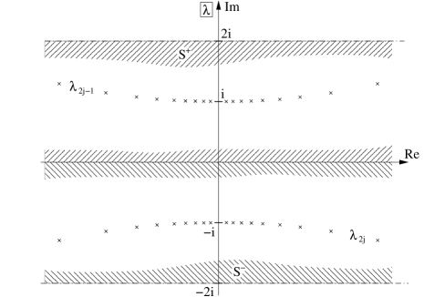
Figure 1: Schematic distribution of the upper and lower Bethe roots $\lambda_{2j-1}$ and $\lambda_{2j}$, respectively, in the strips ${\cal S}^{\pm}$.

Typical physical quantities at finite temperature can be written as sums over the Bethe roots of the dominant state. Such sums can be converted into contour integrals by means of appropriate auxiliary functions having their zeros at the Bethe roots. As compared to the spin-$\frac{1}{2}$ case the choice of the contours and auxiliary functions is more delicate for spin 1. In particular, it seems that the auxiliary functions and integration contours have to be chosen separately in ${\cal S}^{+}$ and ${\cal S}^{-}$. We shall consider the auxiliary functions

$$\mathfrak{f}(\lambda)=\frac{1}{\mathfrak{b}(\lambda-2{\rm i})}\,,\quad\overline{\mathfrak{f}}(\lambda)=\frac{1}{\overline{\mathfrak{b}}(\lambda+2{\rm i})}$$ (50)

(see appendix 7 for the definitions of $\mathfrak{b}$ and $\overline{\mathfrak{b}}$ in terms of $Q$-functions). As usually we also introduce the corresponding ‘capital functions’

$$\mathfrak{F}(\lambda)=1+\mathfrak{f}(\lambda)\,,\quad\overline{\mathfrak{F}}(\lambda)=1+\overline{\mathfrak{f}}(\lambda)\,.$$ (51)

They are meromorphic for finite Trotter number, and $\mathfrak{F}$ has in ${\cal S}^{+}$ exactly $N/2$ zeros located at the upper Bethe roots and only a single $N/2$-fold pole at ${\rm i}-{\rm i}u$. Similarly, $\overline{\mathfrak{F}}$ has in ${\cal S}^{-}$ exactly $N/2$ zeros located at the lower Bethe roots and only a single $N/2$-fold pole at $-{\rm i}+{\rm i}u$.

Using this information and the definitions of some additional useful auxiliary functions in terms of $Q$-functions (see appendix 7) we obtain the following NLIE,

$$\ln\frac{\mathfrak{f}(\lambda)}{\overline{\mathfrak{a}}_{\rm II}(\lambda)} =d_{f}(\lambda)+\ln\frac{\mathfrak{F}(\lambda)}{\overline{\mathfrak{B}}(\lambda)}$$

$$+\int_{{\cal C}^{+}}\frac{{\rm d}\mu}{2\pi{\rm i}}K(\lambda-\mu)\ln\mathfrak{F}(\mu)+\int_{\overline{\cal C}^{-}}\frac{{\rm d}\mu}{2\pi{\rm i}}K(\lambda-\mu)\ln\overline{\mathfrak{F}}(\mu)\,,\quad\lambda\in{\cal C}^{+}\,,$$ (52a)

$$\ln\frac{\overline{\mathfrak{f}}(\lambda)}{\mathfrak{a}_{\rm II}(\lambda)} =-d_{f}(\lambda)+\ln\frac{\overline{\mathfrak{F}}(\lambda)}{\mathfrak{B}(\lambda)}$$

$$-\int_{\overline{\cal C}^{+}}\frac{{\rm d}\mu}{2\pi{\rm i}}K(\lambda-\mu)\ln\mathfrak{F}(\mu)-\int_{{\cal C}^{-}}\frac{{\rm d}\mu}{2\pi{\rm i}}K(\lambda-\mu)\ln\overline{\mathfrak{F}}(\mu)\,,\quad\lambda\in{\cal C}^{-}\,.$$ (52b)

Here we have introduced the kernel

$$K(\lambda)=\frac{1}{\lambda-2{\rm i}}-\frac{1}{\lambda+2{\rm i}}$$ (53)

and the driving term

$$d_{f}(\lambda)=\frac{2h}{T}+\ln\frac{\phi_{+}(\lambda-3{\rm i})\phi_{-}(\lambda-{\rm i})\phi_{-}(\lambda+{\rm i})\phi_{+}(\lambda+3{\rm i})}{\phi_{-}(\lambda-3{\rm i})\phi_{+}(\lambda-{\rm i})\phi_{+}(\lambda+{\rm i})\phi_{-}(\lambda+3{\rm i})}\\[4.30554pt] \overset{N\rightarrow\infty}{\longrightarrow}\ \frac{2h}{T}+\frac{{\rm i}J}{T}\bigl{(}K(\lambda+{\rm i})-K(\lambda-{\rm i})\bigr{)}\,.$$ (54)

Note that the only explicit $N$-dependence is in the driving term $d_{f}$. And since this driving term has a simple Trotter limit, we conclude that the functions $\mathfrak{f}$ and $\overline{\mathfrak{f}}$ have a Trotter limit as well.

Figure 2: The contours ${\cal C}^{\pm}$ in the strips ${\cal S}^{\pm}$ encircle the upper and lower Bethe roots respectively and close at infinity.

The precise definition of the integration contours is slightly subtle. We illustrate it in figure 2. ${\cal C}^{+}$ is a simple closed contour inside ${\cal S}^{+}$ that encircles the upper Bethe roots. We may realize it as a large rectangle with upper edge slightly below $2{\rm i}$ and lower edge slightly above the real axis. Similarly ${\cal C}^{-}$ must enclose the lower Bethe roots inside ${\cal S}^{-}$ and may also be taken as a large rectangle, now with lower edge slightly above $-2{\rm i}$ and with upper edge slightly below the real axis. The bar in $\overline{\cal C}^{\pm}$ means that the contours do not encircle the singularities originating from the kernel $K(\lambda)$. This prescription may be seen as an ‘${\rm i}\varepsilon$-regularization’ of the kernel after the contour integral is decomposed into an integral over straight lines. Such type of regularization is needed because the kernel has poles at $\mu=\lambda\pm 2{\rm i}$ which must not lie on the contours. Having in mind the multiple integral representation in the next section we prefer to realize it in the way sketched in figure 3, where $\overline{\cal C}^{+}-2{\rm i}$ inside $\overline{\cal C}^{-}={\cal C}^{-}$ inside ${\cal C}^{+}-2{\rm i}$, and ‘inside’ means ‘infinitesimally narrower’.

At first sight, (52a) and (52b) do not seem to be enough to fix the unknown functions, as the number of equations is smaller than that of the functions. In order to understand that they actually fix the functions $\mathfrak{f}$ and $\overline{\mathfrak{f}}$, let us simulate one step in the iterative scheme. Assume that an approximate estimation of $\mathfrak{f},\overline{\mathfrak{f}}$ is already known. Then $\mathfrak{a}_{\rm II}$, $\overline{\mathfrak{a}}_{\rm II}$ are determined from $\mathfrak{f},\overline{\mathfrak{f}}$ by

$$\mathfrak{a}_{\rm II}(\lambda)=\frac{\frac{1}{\mathfrak{f}(\lambda+2{\rm i})}-\overline{\mathfrak{f}}(\lambda)}{\overline{\mathfrak{F}}(\lambda)}\,,\ \text{for $\lambda\in{\cal C}^{-}$,}\quad\overline{\mathfrak{a}}_{\rm II}(\lambda)=\frac{\frac{1}{\overline{\mathfrak{f}}(\lambda-2{\rm i})}-\mathfrak{f}(\lambda)}{\mathfrak{F}(\lambda)}\,,\ \text{for $\lambda\in{\cal C}^{+}$.}$$ (55)

Figure 3: For the regularization in the multiple integral representation the dashed lines show the relative positions of the contours ${\cal C}^{\pm}$, $\overline{\cal C}^{\pm}$.

Note that ${\overline{\mathfrak{B}}(\lambda)}/{\mathfrak{F}(\lambda)}$ and ${\mathfrak{B}(\lambda)}/{\overline{\mathfrak{F}}(\lambda)}$ are equal to $1+\overline{\mathfrak{a}}_{\rm II}(\lambda)$ and $1+\mathfrak{a}_{\rm II}(\lambda)$, respectively. They are thus determined by given $\mathfrak{f},\overline{\mathfrak{f}}$. Substituting them into the rhs of (52a) and (52b) (and $\mathfrak{a}_{\rm II},\overline{\mathfrak{a}}_{\rm II}$ into the lhs), we obtain the next-step approximation to $\mathfrak{f},\overline{\mathfrak{f}}$. Therefore equations (52) consistently fix $\mathfrak{f}$ and $\overline{\mathfrak{f}}$. The other functions are then determined from them.

Suppose that we have evaluated the auxiliary functions through (52). Then, for $|{\rm Im\,}\lambda|<1$, the largest eigenvalue $\Lambda^{[2]}(\lambda)$ is obtained as

$$\ln\Lambda^{[2]}(\lambda) =\ln\Lambda^{[2]}_{0}(\lambda)+\int_{{\cal C}^{-}}\frac{{\rm d}\mu}{2\pi{\rm i}}K(\lambda-\mu-3{\rm i})\ln\mathfrak{B}(\mu)+\int_{{\cal C}^{+}}\frac{{\rm d}\mu}{2\pi{\rm i}}K(\lambda-\mu+{\rm i})\ln\overline{\mathfrak{B}}(\mu)\,,$$

$$\ln\Lambda^{[2]}_{0}(\lambda) =\frac{2h}{T}+\ln\frac{\phi_{+}(\lambda-2{\rm i})\phi_{-}(\lambda+2{\rm i})}{\phi_{-}(\lambda-2{\rm i})\phi_{+}(\lambda+2{\rm i})}\ \overset{N\rightarrow\infty}{\longrightarrow}\ \frac{2h}{T}+\frac{4J}{T}\frac{1}{\lambda^{2}+4}\,.$$ (56)

The NLIE (52) are actually only one of many possible choices. We choose this one as we think that it has an advantage compared to others in the following sense. Although the equations themselves are literally correct, the integrations over contours suffer from poor numerical accuracy, especially in the low temperature regime. Therefore it is better to rewrite them in the form obtained in [30], where the integrations are defined on the straight lines. We will show in appendix 7 that (52) can be transformed into (58) below with the help of additional algebraic relations among the auxiliary functions. In the same appendix 7 we also provide subsidiary equations that determine the functions $\mathfrak{f}$, $\overline{\mathfrak{f}}$ on straight lines close to the real axis, which amounts to knowing $\mathfrak{b}$ and $\overline{\mathfrak{b}}$ on straight lines close to $\pm 2{\rm i}$ (see (50)).

Unlike in (52) we need to deal with $\mathfrak{b}(\lambda),\overline{\mathfrak{b}}(\lambda)$ and $y(\lambda)$, if we choose straight lines as integration contours. For convenience we introduce the shifted functions

$$\mathfrak{b}_{\epsilon}(\lambda)=\mathfrak{b}(\lambda-{\rm i}\epsilon)\,,\quad\overline{\mathfrak{b}}_{\epsilon}(\lambda)=\overline{\mathfrak{b}}(\lambda+{\rm i}\epsilon)\,,$$ (57)

and similar capital functions. Then the desired NLIE read

$$\begin{pmatrix}\log y(\lambda)\\ \log\mathfrak{b}_{\epsilon}(\lambda)\\ \log\overline{\mathfrak{b}}_{\epsilon}(\lambda)\end{pmatrix}=\begin{pmatrix}0\\ \Delta_{b}(\lambda)\\ \Delta_{\overline{b}}(\lambda)\end{pmatrix}+\widehat{\cal K}*\begin{pmatrix}\log Y(\lambda)\\ \log\mathfrak{B}_{\epsilon}(\lambda)\\ \log\overline{\mathfrak{B}}_{\epsilon}(\lambda)\end{pmatrix}\,,$$ (58)

where $(\widehat{\cal K}*g)_{i}$ denotes the matrix convolution $\sum_{j}\int_{-\infty}^{\infty}{\rm d}\mu\,\widehat{\cal K}_{i,j}(\lambda-\mu)g_{j}(\mu)$, and

$$\Delta_{b}(\lambda) =-\frac{h}{T}+d(u,\lambda-{\rm i}\epsilon)\,,\quad\Delta_{\overline{b}}(\lambda)=\frac{h}{T}+d(u,\lambda+{\rm i}\epsilon)\,,$$ (59a)

$$d(u,\lambda) =\frac{N}{2}\int_{-\infty}^{\infty}{\rm d}k\,{\rm e}^{-{\rm i}k\lambda}\frac{\sinh uk}{k\cosh k}\ \overset{N\rightarrow\infty}{\longrightarrow}\ -\frac{J}{T}\frac{\pi}{2\cosh\pi\lambda/2}\,.$$ (59b)

The integration constants ($\pm h/T$) are fixed by comparing the asymptotic values of both sides of (58) for $|\lambda|\rightarrow\infty$. The kernel matrix is given by

$$\widehat{\cal{\cal K}}(\lambda)=\begin{pmatrix}0&{\cal K}(\lambda+{\rm i}\epsilon)&{\cal K}(\lambda-{\rm i}\epsilon)\\ {\cal K}(\lambda-{\rm i}\epsilon)&{\cal F}(\lambda)&-{\cal F}(\lambda+2{\rm i}(1-\epsilon))\\ {\cal K}(\lambda+{\rm i}\epsilon)&-{\cal F}(\lambda-2{\rm i}(1-\epsilon))&{\cal F}(\lambda)\end{pmatrix}\,,$$ (60)

where

$${\cal K}(\lambda)=\frac{1}{4\cosh\pi\lambda/2}\,,\quad{\cal F}(\lambda)=\int_{-\infty}^{\infty}\frac{{\rm d}k}{2\pi}\,\frac{e^{-|k|-{\rm i}k\lambda}}{2\cosh k}\,.$$ (61)

The free energy then follows from (24) noticing that the dominant eigenvalue can be represented by integration over straight lines as

$$\ln\Lambda^{[2]}(\lambda)=\ln\Lambda^{[2]}_{0}(\lambda)-\frac{2h}{T}\\ +\int_{-\infty}^{\infty}{\rm d}\mu\;{\cal K}(\lambda-\mu+{\rm i}\varepsilon)\ln\mathfrak{B}_{\epsilon}(\mu)+\int_{-\infty}^{\infty}{\rm d}\mu\;{\cal K}(\lambda-\mu-{\rm i}\varepsilon)\ln\overline{\mathfrak{B}}_{\epsilon}(\mu)\,.$$ (62)

As the actual transformation from (52) to (58) is involved, we defer the details to appendix 7.

4 The multiple integral representation

In this section we present the main result of this work, which is a multiple integral formula for the matrix elements ${D^{[2]}}^{\alpha_{1},\dots,\alpha_{m}}_{\beta_{1},\dots,\beta_{m}}(\xi)$, $\alpha_{j},\beta_{k}=-,0,+$, of the inhomogeneous density matrix (27). Our formula generalizes the result of [21] to finite temperature and magnetic field and the result of [14] to spin 1. The details of the derivation can be found in appendix 7.

For any two sequences $(\alpha)=(\alpha_{n})_{n=1}^{m}$ and $(\beta)=(\beta_{n})_{n=1}^{m}$ of upper and lower matrix indices we shall obtain a different multiple integral. Let us introduce the notation $n_{\sigma}(x)$, $\sigma=-,0,+$, $(x)=(\alpha),(\beta)$, for the number of $\sigma$s in the sequence $(x)$, e.g. $n_{0}(\beta)$ is the number of zeros in $(\beta)$. Then

$$n_{+}(\alpha)+n_{0}(\alpha)+n_{-}(\alpha)=m\,,$$ (63a)

$$n_{+}(\beta)+n_{0}(\beta)+n_{-}(\beta)=m\,,$$ (63b)

$$n_{+}(\beta)-n_{-}(\beta)-n_{+}(\alpha)+n_{-}(\alpha)=0\,.$$ (63c)

Here the last equation is equivalent to $2n_{+}(\alpha)+n_{0}(\alpha)=2n_{+}(\beta)+n_{0}(\beta)$.

The dependence of the multiple integral on the indices $\alpha_{j}$, $\beta_{k}$ enters through a sequence $(z)=(z_{n})_{n=1}^{2m}$ encoding the positions of $-,0,+$ in $(\alpha)$ and $(\beta)$. For the construction of $(z)$ we order the density matrix indices as $\alpha_{m},\dots,\alpha_{1},\beta_{1},\dots,\beta_{m}$ and inspect them starting from the left. If $\alpha_{m}=-$ we do nothing, if $\alpha_{m}=0$ we define $z_{1}=m$, and if $\alpha_{m}=+$ we define $z_{1}=z_{2}=m$. We continue this procedure with $\alpha_{m-1}$ and so on. When we have reached $\alpha_{1}$ we have defined

$$p=2n_{+}(\alpha)+n_{0}(\alpha)$$ (64)

elements of the sequence $(z)$ in this way. If $\beta_{1}=-$ we define $z_{p+1}=z_{p+2}=1$, if $\beta_{1}=0$ we define $z_{p+1}=1$, and if $\beta_{1}=+$ we do nothing. We continue the same way with $\beta_{2}$, $\beta_{3}$ etc. until we end at $\beta_{m}$. The sequence $(z)$ thus constructed has $2n_{+}(\alpha)+n_{0}(\alpha)+n_{0}(\beta)+2n_{-}(\beta)=2m$ elements, and the pair $(z)$, $p$ is in one-to-one correspondence with the sequences $(\alpha)$ and $(\beta)$. As an example let us consider $(\alpha)=(+,-,0),\beta=(0,0,0)$. Then $z_{1}=3$, $z_{2}=z_{3}=z_{4}=1$, $z_{5}=2$, $z_{6}=3$, $p=3$.

Two types of functions occur under the multiple integral. One type is explicit and has its origin in the Yang-Baxter algebra. The functions

$$F_{\ell}(\lambda) =\prod_{k=1}^{m}(\lambda-\xi_{k}-{\rm i})\>\prod_{k=1}^{\ell-1}(\lambda-\xi_{k}-3{\rm i})\prod_{k=\ell+1}^{m}(\lambda-\xi_{k}+{\rm i})\,,$$ (65a)

$$\overline{F}_{\ell}(\lambda) =\prod_{k=1}^{m}(\lambda-\xi_{k}+{\rm i})\>\prod_{k=1}^{\ell-1}(\lambda-\xi_{k}+3{\rm i})\prod_{k=\ell+1}^{m}(\lambda-\xi_{k}-{\rm i})$$ (65b)

belong to this type. We think of them as ‘fused wave functions’.

The other type is related to the task of rewriting sums over Bethe roots as integrals over closed contours (see appendix 7). These functions may be defined as solutions of linear integral equations over closed contours. We have two pairs of such functions. The first one is defined by

$$G^{+}(\lambda,\xi)=K(\lambda-\xi-3{\rm i})-K(\lambda-\xi-{\rm i})$$

$$\mspace{18.0mu}-\int_{{\cal C}^{+}}\frac{{\rm d}\mu}{2\pi{\rm i}}\frac{\mathfrak{F}(\mu)}{\overline{\mathfrak{B}}(\mu)}G^{+}(\mu,\xi)K(\lambda-\mu)+\int_{\overline{\cal C}^{-}}\frac{{\rm d}\mu}{2\pi{\rm i}}\frac{\overline{\mathfrak{F}}(\mu)}{\mathfrak{B}(\mu)}G^{-}(\mu,\xi)K(\lambda-\mu-4{\rm i})\,,$$ (66a)

$$G^{-}(\lambda,\xi)=K(\lambda-\xi+{\rm i})-K(\lambda-\xi+3{\rm i})$$

$$\mspace{18.0mu}-\int_{\overline{\cal C}^{+}}\frac{{\rm d}\mu}{2\pi{\rm i}}\frac{\mathfrak{F}(\mu)}{\overline{\mathfrak{B}}(\mu)}G^{+}(\mu,\xi)K(\lambda-\mu+4{\rm i})+\int_{{\cal C}^{-}}\frac{{\rm d}\mu}{2\pi{\rm i}}\frac{\overline{\mathfrak{F}}(\mu)}{\mathfrak{B}(\mu)}G^{-}(\mu,\xi)K(\lambda-\mu)\,,$$ (66b)

where $\lambda\in{\cal C}^{+}$ for $G^{+}$ and $\lambda\in{\cal C}^{-}$ for $G^{-}$. The second pair of auxiliary functions needed in the definition of the multiple integral is

$$S^{+}(\lambda,\xi)=-{\rm e}(\lambda-\xi-5{\rm i})-{\rm e}(\lambda-\xi-{\rm i})-\frac{1}{Y(\xi)}\bigl{(}K(\lambda-\xi-3{\rm i})+K(\lambda-\xi-{\rm i})\bigr{)}$$

$$\mspace{18.0mu}-\int_{{\cal C}^{+}}\frac{{\rm d}\mu}{2\pi{\rm i}}\frac{\mathfrak{F}(\mu)}{\overline{\mathfrak{B}}(\mu)}S^{+}(\mu,\xi)K(\lambda-\mu)+\int_{\overline{\cal C}^{-}}\frac{{\rm d}\mu}{2\pi{\rm i}}\frac{\overline{\mathfrak{F}}(\mu)}{\mathfrak{B}(\mu)}S^{-}(\mu,\xi)K(\lambda-\mu-4{\rm i})\,,$$ (67a)

$$S^{-}(\lambda,\xi)=-{\rm e}(\lambda-\xi-{\rm i})-{\rm e}(\lambda-\xi+3{\rm i})-\frac{1}{Y(\xi)}\bigl{(}K(\lambda-\xi+{\rm i})+K(\lambda-\xi+3{\rm i})\bigr{)}$$

$$\mspace{18.0mu}-\int_{\overline{\cal C}^{+}}\frac{{\rm d}\mu}{2\pi{\rm i}}\frac{\mathfrak{F}(\mu)}{\overline{\mathfrak{B}}(\mu)}S^{+}(\mu,\xi)K(\lambda-\mu+4{\rm i})+\int_{{\cal C}^{-}}\frac{{\rm d}\mu}{2\pi{\rm i}}\frac{\overline{\mathfrak{F}}(\mu)}{\mathfrak{B}(\mu)}S^{-}(\mu,\xi)K(\lambda-\mu)\,,$$ (67b)

where, similar to the above case, $\lambda\in{\cal C}^{+}$ for $S^{+}$ and $\lambda\in{\cal C}^{-}$ for $S^{-}$ and where we have introduced the ‘bare energy function’

$${\rm e}(\lambda)=\frac{1}{\lambda}-\frac{1}{\lambda+2{\rm i}}\,.$$ (68)

The functions $G^{\pm}$ and $S^{\pm}$ enter the multiple integral through the determinant of a matrix with elements $\Theta_{j,k}^{(p)}$ defined by

$$\Theta_{j,2k-1}^{(p)} =\begin{cases}G^{+}(\omega_{j},\xi_{k})&j=1,\dots,p\\ G^{-}(\omega_{j},\xi_{k})&j=p+1,\dots,2m\,,\end{cases}$$ (69a)

$$\Theta_{j,2k}^{(p)} =\begin{cases}{\rm i}S^{+}(\omega_{j},\xi_{k})&j=1,\dots,p\\ {\rm i}S^{-}(\omega_{j},\xi_{k})&j=p+1,\dots,2m\,.\end{cases}$$ (69b)

Using all of the above defined notation we can write the non-vanishing matrix elements of the inhomogeneous spin-1 density matrix as

$${D^{[2]}}^{\alpha_{1},\dots,\alpha_{m}}_{\beta_{1},\dots,\beta_{m}}(\xi)=\frac{2^{-m-n_{+}(\alpha)-n_{-}(\beta)}}{\prod_{1\leq j<k\leq m}(\xi_{k}-\xi_{j})^{2}[(\xi_{k}-\xi_{j})^{2}+4]}\\[4.30554pt] \biggl{[}\prod_{j=1}^{p}\int_{\cal C}\frac{{\rm d}\omega_{j}}{2\pi{\rm i}}F_{z_{j}}(\omega_{j})\biggr{]}\biggl{[}\prod_{j=p+1}^{2m}\int_{\overline{\cal C}}\frac{{\rm d}\omega_{j}}{2\pi{\rm i}}\overline{F}_{z_{j}}(\omega_{j})\biggr{]}\frac{\det_{2m}\Theta^{(p)}_{j,k}}{\prod_{1\leq j<k\leq 2m}(\omega_{j}-\omega_{k}-2{\rm i})}\,.$$ (70)

This formula is the main result of our work. It represents the inhomogeneous density matrix of the integrable spin-1 chain as a single multiple integral. All dependence on the Trotter number has been absorbed into the auxiliary functions $G^{\pm}$ and $S^{\pm}$. Therefore the Trotter limit is trivial in this formulation.

Note that it is also easy to perform the homogenous limit. In complete analogy with the spin-$\frac{1}{2}$ case [24, 14] we obtain

$${D_{[1,m]}}^{\alpha_{1},\dots,\alpha_{m}}_{\beta_{1},\dots,\beta_{m}}(T,h)=2^{-m^{2}-n_{+}(\alpha)-n_{-}(\beta)}\\ \biggl{[}\prod_{j=1}^{p}\int_{\cal C}\frac{{\rm d}\omega_{j}}{2\pi{\rm i}}F_{z_{j}}(\omega_{j})\biggr{]}\biggl{[}\prod_{j=p+1}^{2m}\int_{\overline{\cal C}}\frac{{\rm d}\omega_{j}}{2\pi{\rm i}}\overline{F}_{z_{j}}(\omega_{j})\biggr{]}\frac{\det_{2m}\Xi^{(p)}_{j,k}}{\prod_{1\leq j<k\leq 2m}(\omega_{j}-\omega_{k}-2{\rm i})}$$ (71)

for the physical density matrix. Here we introduced the notation

$$\Xi_{j,2k-1}^{(p)} =\frac{\partial_{\xi}^{k-1}}{(k-1)!}\begin{cases}G^{+}(\omega_{j},\xi)|_{\xi=0}&j=1,\dots,p\\ G^{-}(\omega_{j},\xi)|_{\xi=0}&j=p+1,\dots,2m\,,\end{cases}$$ (72a)

$$\Xi_{j,2k}^{(p)} =\frac{{\rm i}\,\partial_{\xi}^{k-1}}{(k-1)!}\begin{cases}S^{+}(\omega_{j},\xi)|_{\xi=0}&j=1,\dots,p\\ S^{-}(\omega_{j},\xi)|_{\xi=0}&j=p+1,\dots,2m\,.\end{cases}$$ (72b)

5 One-point functions in factorized form

In this section we have a closer look at the one-point functions which are the most elementary correlation functions. Using the general multiple integral formula (70) we can write the non-zero one-point functions as

$$D^{+}_{+}(\xi) =\frac{{\rm i}}{4}\int_{\cal C}\frac{{\rm d}\omega_{1}}{2\pi{\rm i}}\int_{\cal C}\frac{{\rm d}\omega_{2}}{2\pi{\rm i}}\frac{(\omega_{1}-\xi-{\rm i})(\omega_{2}-\xi-{\rm i})}{\omega_{1}-\omega_{2}-2{\rm i}}\biggl{|}\begin{array}[]{cc}G^{+}(\omega_{1},\xi)&S^{+}(\omega_{1},\xi)\\ G^{+}(\omega_{2},\xi)&S^{+}(\omega_{2},\xi)\end{array}\biggr{|}\,,$$ (75)

$$D^{0}_{0}(\xi) =\frac{{\rm i}}{2}\int_{\cal C}\frac{{\rm d}\omega_{1}}{2\pi{\rm i}}\int_{\overline{\cal C}}\frac{{\rm d}\omega_{2}}{2\pi{\rm i}}\frac{(\omega_{1}-\xi-{\rm i})(\omega_{2}-\xi+{\rm i})}{\omega_{1}-\omega_{2}-2{\rm i}}\biggl{|}\begin{array}[]{cc}G^{+}(\omega_{1},\xi)&S^{+}(\omega_{1},\xi)\\ G^{-}(\omega_{2},\xi)&S^{-}(\omega_{2},\xi)\end{array}\biggr{|}\,,$$ (78)

$$D^{-}_{-}(\xi) =\frac{{\rm i}}{4}\int_{\overline{\cal C}}\frac{{\rm d}\omega_{1}}{2\pi{\rm i}}\int_{\overline{\cal C}}\frac{{\rm d}\omega_{2}}{2\pi{\rm i}}\frac{(\omega_{1}-\xi+{\rm i})(\omega_{2}-\xi+{\rm i})}{\omega_{1}-\omega_{2}-2{\rm i}}\biggl{|}\begin{array}[]{cc}G^{-}(\omega_{1},\xi)&S^{-}(\omega_{1},\xi)\\ G^{-}(\omega_{2},\xi)&S^{-}(\omega_{2},\xi)\end{array}\biggr{|}\,.$$ (81)

This is the double integral form of the one-point functions. Judging from our experience with the spin-$\frac{1}{2}$ case [7, 3] and with the spin-1 ground state correlation functions [21] we expect these integrals to factorize into sums over products of single integrals.

This is indeed the case. For $n=0,1$ we introduce the following functions represented by single integrals,

$$\sigma_{n}(\xi) =\int_{{\cal C}^{+}}\frac{{\rm d}\lambda}{2\pi{\rm i}}\frac{\mathfrak{F}(\lambda)}{\overline{\mathfrak{B}}(\lambda)}\lambda^{n}G^{+}(\lambda,\xi)-\int_{{\cal C}^{-}}\frac{{\rm d}\lambda}{2\pi{\rm i}}\frac{\overline{\mathfrak{F}}(\lambda)}{\mathfrak{B}(\lambda)}\lambda^{n}G^{-}(\lambda,\xi)\,,$$ (82a)

$$\delta_{n}(\xi) =\int_{{\cal C}^{+}}\frac{{\rm d}\lambda}{2\pi{\rm i}}\frac{\mathfrak{F}(\lambda)}{\overline{\mathfrak{B}}(\lambda)}\lambda^{n}S^{+}(\lambda,\xi)-\int_{{\cal C}^{-}}\frac{{\rm d}\lambda}{2\pi{\rm i}}\frac{\overline{\mathfrak{F}}(\lambda)}{\mathfrak{B}(\lambda)}\lambda^{n}S^{-}(\lambda,\xi)\,.$$ (82b)

Then, using tricks similar to those employed in [3], we obtain the ‘magnetization’

$$D^{+}_{+}(\xi)-D^{-}_{-}(\xi)=\sigma_{0}(\xi)$$ (83)

and the ‘probability for measuring zero for the $z$-component of the spin’,

$$D^{0}_{0}(\xi)=\frac{1}{3}-\frac{{\rm i}}{3}\left|\begin{array}[]{cc}\sigma_{0}(\xi)&\sigma_{1}(\xi)-2{\rm i}\\[8.61108pt] \delta_{0}(\xi)+1+\frac{2}{Y(\xi)}&\delta_{1}(\xi)+\xi\Bigl{(}1+\frac{2}{Y(\xi)}\Bigr{)}\end{array}\right|\,,$$ (84)

in factorized form. They determine all one-point functions because of the relation

$$D^{+}_{+}(\xi)+D^{0}_{0}(\xi)+D^{-}_{-}(\xi)=1\,.$$ (85)

Note that $\sigma_{0}$ and also the whole determinant in (84) must vanish for symmetry reasons if the magnetic field is switched off.

6 The zero temperature limit at vanishing magnetic field

All dependence on temperature of the multiple integral formula (70) is hidden in the functions $G^{\pm}$ and $S^{\pm}$. We obtain the ground state result for vanishing magnetic field by replacing these functions by their corresponding limits which have to be calculated from (66), (67).

The temperature enters these equations through the functions $\mathfrak{b}$, $\overline{\mathfrak{b}}$, $\mathfrak{f}$, $\overline{\mathfrak{f}}$ and $y$. How do they behave in the limit? We first look at the nonlinear integral equations (58). As $T\rightarrow 0$ for $h=0$, the driving terms in the equations for $\mathfrak{b}$ and $\overline{\mathfrak{b}}$ both go to minus infinity pointwise. It follows that $\mathfrak{b},\overline{\mathfrak{b}}\rightarrow 0$ on lines slightly below or slightly above the real axis. From the equation for $y$ we conclude that $y\rightarrow 1$ close to the real axis. Then by equation (B.16) also $y(\lambda\pm{\rm i})\rightarrow 1$ for $\lambda$ close to the real axis, and, using (B.15), we find that $\mathfrak{f},\overline{\mathfrak{f}}\rightarrow 0$. Thus,

$$\lim_{T\rightarrow 0+}\lim_{h\rightarrow 0}\frac{\overline{\mathfrak{F}}(\lambda)}{\mathfrak{B}(\lambda)}=1\,,\quad\lim_{T\rightarrow 0+}\lim_{h\rightarrow 0}\frac{\mathfrak{F}(\lambda)}{\overline{\mathfrak{B}}(\lambda)}=1$$ (86)

for $\lambda$ slightly below or above the real axis. The behaviour of these functions close to the lower edge of ${\cal C}^{-}$ and close to the upper edge of ${\cal C}^{+}$ then follows from (A.9b),

$$\lim_{T\rightarrow 0+}\lim_{h\rightarrow 0}\frac{\overline{\mathfrak{F}}(\lambda-2{\rm i})}{\mathfrak{B}(\lambda-2{\rm i})}=\frac{1}{2}\,,\quad\lim_{T\rightarrow 0+}\lim_{h\rightarrow 0}\frac{\mathfrak{F}(\lambda+2{\rm i})}{\overline{\mathfrak{B}}(\lambda+2{\rm i})}=\frac{1}{2}$$ (87)

for $\lambda$ slightly above or below the real axis.

Inserting (86) and (87) into (66) and (67) and using that $Y(\xi)\rightarrow 2$ we obtain a set of linear integral equations of convolution type that can be solved by means of Fourier transformation. Some care is required with the relative location of the contours, though. Referring to the notation

$$Z^{++}(\lambda,\xi)=\lim_{\varepsilon\rightarrow 0+}\lim_{T\rightarrow 0+}\lim_{h\rightarrow 0}Z^{+}(\lambda+2{\rm i}-{\rm i}\varepsilon,\xi)\,,$$ (88a)

$$Z^{+-}(\lambda,\xi)=\lim_{\varepsilon\rightarrow 0+}\lim_{T\rightarrow 0+}\lim_{h\rightarrow 0}Z^{+}(\lambda+{\rm i}\varepsilon,\xi)\,,$$ (88b)

$$Z^{-+}(\lambda,\xi)=\lim_{\varepsilon\rightarrow 0+}\lim_{T\rightarrow 0+}\lim_{h\rightarrow 0}Z^{-}(\lambda-{\rm i}\varepsilon,\xi)\,,$$ (88c)

$$Z^{--}(\lambda,\xi)=\lim_{\varepsilon\rightarrow 0+}\lim_{T\rightarrow 0+}\lim_{h\rightarrow 0}Z^{-}(\lambda-2{\rm i}+{\rm i}\varepsilon,\xi)\,,$$ (88d)

where $Z=G$ or $Z=S$, we obtain the following results

$$G^{++}(\lambda,\xi)=G^{--}(\lambda,\xi)=0\,,$$ (89a)

$$G^{-+}(\lambda,\xi)=-G^{+-}(\lambda,\xi)=\frac{{\rm i}\pi}{2\operatorname{ch}\bigl{(}\frac{\pi}{2}(\lambda-\xi)\bigr{)}}\,,$$ (89b)

$$S^{++}(\lambda,\xi)=S^{--}(\lambda,\xi)=\frac{{\rm i}\pi}{\operatorname{ch}\bigl{(}\frac{\pi}{2}(\lambda-\xi)\bigr{)}}\,,$$ (89c)

$$S^{-+}(\lambda,\xi)=\frac{\pi(\lambda-\xi-2{\rm i})}{4\operatorname{ch}\bigl{(}\frac{\pi}{2}(\lambda-\xi)\bigr{)}}\,,\quad S^{+-}(\lambda,\xi)=\frac{-\pi(\lambda-\xi+2{\rm i})}{4\operatorname{ch}\bigl{(}\frac{\pi}{2}(\lambda-\xi)\bigr{)}}\,.$$ (89d)

As a first consistency test we may insert these results into our formulae (82) for the one-point functions. We obtain $\sigma_{0}=0$ and $\delta_{0}=-2$. Then (83), (84) and (85) imply that $D^{+}_{+}(0)=D^{0}_{0}(0)=D^{-}_{-}(0)=1/3$ as it must be from symmetry considerations. This is, of course, in agreement with [21].

Still, it is not obvious how to relate, in general, the limit of our multiple integral to the multiple integral derived there directly for the ground state at vanishing field. Here we consider only the case of the one-point functions and defer any further discussion to future work. We have to calculate the limits of $G^{+}$ and $S^{+}$ in the lower strip ${\cal S}^{-}$ and the limits of $G^{-}$ and $S^{-}$ in the upper strip ${\cal S}^{+}$ on lines close to the real axis and close to $\pm 2{\rm i}$. These lines must be chosen in such a way that all poles of the kernels in (66), (67) are located outside the integration contours. Keeping this in mind we define

$$Z_{++}(\lambda,\xi)=\lim_{\varepsilon\rightarrow 0+}\lim_{T\rightarrow 0+}\lim_{h\rightarrow 0}Z^{+}(\lambda-{\rm i}\varepsilon,\xi)\,,$$ (90a)

$$Z_{+-}(\lambda,\xi)=\lim_{\varepsilon\rightarrow 0+}\lim_{T\rightarrow 0+}\lim_{h\rightarrow 0}Z^{+}(\lambda-2{\rm i}+{\rm i}\varepsilon,\xi)\,,$$ (90b)

$$Z_{-+}(\lambda,\xi)=\lim_{\varepsilon\rightarrow 0+}\lim_{T\rightarrow 0+}\lim_{h\rightarrow 0}Z^{-}(\lambda+2{\rm i}-{\rm i}\varepsilon,\xi)\,,$$ (90c)

$$Z_{--}(\lambda,\xi)=\lim_{\varepsilon\rightarrow 0+}\lim_{T\rightarrow 0+}\lim_{h\rightarrow 0}Z^{-}(\lambda+{\rm i}\varepsilon,\xi)\,,$$ (90d)

for $Z=G$ and $Z=S$. Inserting (89) into (66), (67) we obtain

$$G_{-+}(\lambda,\xi)=G_{+-}(\lambda,\xi)=0\,,$$ (91a)

$$S_{-+}(\lambda,\xi)=S_{+-}(\lambda,\xi)=0\,,$$ (91b)

$$G_{--}(\lambda,\xi)=-G_{++}(\lambda,\xi)=\frac{{\rm i}\pi}{2\operatorname{ch}\bigl{(}\frac{\pi}{2}(\lambda-\xi)\bigr{)}}\,,$$ (91c)

$$S_{--}(\lambda,\xi)=\frac{\pi(\lambda-\xi-2{\rm i})}{4\operatorname{ch}\bigl{(}\frac{\pi}{2}(\lambda-\xi)\bigr{)}}\,,\quad S_{++}(\lambda,\xi)=\frac{-\pi(\lambda-\xi+2{\rm i})}{4\operatorname{ch}\bigl{(}\frac{\pi}{2}(\lambda-\xi)\bigr{)}}\,.$$ (91d)

Inserting (89) and (91) into (75), in turn, we arrive at

$$D^{+}_{+}(0)= D^{-}_{-}(0)=$$

$$= \frac{{\rm i}}{4}\int_{-\infty}^{\infty}\frac{{\rm d}x_{1}}{\operatorname{ch}({\pi x_{1}})}\int_{-\infty}^{\infty}\frac{{\rm d}x_{2}}{\operatorname{ch}({\pi x_{2}})}\left[\frac{(x_{1}+\frac{{\rm i}}{2})(x_{2}-\frac{{\rm i}}{2})}{x_{1}-x_{2}+{\rm i}0}-\frac{(x_{1}+\frac{{\rm i}}{2})(x_{2}-\frac{{\rm i}}{2})}{x_{1}-x_{2}-{\rm i}0}\right]$$

$$= \frac{{\rm i}}{4}\int_{-\infty}^{\infty}\frac{{\rm d}x_{1}}{\operatorname{ch}({\pi x_{1}})}\int_{-\infty}^{\infty}\frac{{\rm d}x_{2}}{\operatorname{ch}({\pi x_{2}})}\left[\frac{(x_{1}+\frac{{\rm i}}{2})(x_{2}-\frac{{\rm i}}{2})}{x_{1}-x_{2}+{\rm i}0}-\frac{(x_{1}-\frac{{\rm i}}{2})(x_{2}+\frac{{\rm i}}{2})}{x_{1}-x_{2}-2{\rm i}}\right]$$

$$= \frac{\pi}{2}\int_{-\infty}^{\infty}{\rm d}x\;\frac{x^{2}+\frac{1}{4}}{\operatorname{ch}^{2}(\pi x)}=\frac{1}{3}\,,$$ (92)

to be compared with (4.9) and (4.13) of Kitanine [21]. Similarly, (4.12) of [21] for $D^{0}_{0}(0)$ is reproduced as well,

$$D^{0}_{0}(0)= \frac{{\rm i}}{2}\int_{-\infty}^{\infty}\frac{{\rm d}x_{1}}{\operatorname{ch}({\pi x_{1}})}\int_{-\infty}^{\infty}\frac{{\rm d}x_{2}}{\operatorname{ch}({\pi x_{2}})}\left[\frac{(x_{1}+\frac{{\rm i}}{2})(x_{2}+\frac{{\rm i}}{2})}{x_{1}-x_{2}-{\rm i}0}-\frac{(x_{1}+\frac{{\rm i}}{2})(x_{2}+\frac{{\rm i}}{2})}{x_{1}-x_{2}+{\rm i}0}\right]$$

$$= \frac{\pi}{2}\int_{-\infty}^{\infty}{\rm d}x\;\frac{\frac{1}{2}-2x^{2}}{\operatorname{ch}^{2}(\pi x)}=\frac{1}{3}\,.$$ (93)

7 Conclusion

We have managed to represent the inhomogeneous density matrix of the integrable isotropic spin-$1$ chain as a single multiple integral (70). Our formula admits of the Trotter limit, the homogeneous limit and the zero temperature and zero magnetic field limit, where it reproduces the known values of the one-point functions. The main difficulty in the derivation of (70) was not in the algebraic part, which can be treated in a similar way as in the ground state case, but in the analytic part. For finite temperature we can not work with root density functions. Instead, the integrals are obtained by replacing sums over Bethe roots by integrals over closed contours encircling the Bethe roots. In the spin-$1$ case the Bethe roots for the dominant state of the quantum transfer matrix come in widely separated pairs, so-called two-strings. In the Trotter limit they cluster close to $\pm{\rm i}$. Therefore, in order to avoid unwanted extra-terms, we were forced to introduce closed contours consisting of two separated loops, which brought about a considerable amount of technical complexity into the derivation as compared to the spin-$\frac{1}{2}$ case [12] (see appendix 7).

We believe that our result can be generalized to the critical anisotropic case, as it was done for the ground state at vanishing magnetic field in [10], and to arbitrary higher spins. Of particular interest for our own research will be the question if the correlation functions of the integrable higher spin chains factorize. We have obtained a first hint in this direction: we saw in section 5 that the integrals for the one-point functions factorize. This is still not what was called factorization of correlation functions in [4] and what was recently proved to hold for the spin-$\frac{1}{2}$ XXZ chain, namely, that all correlation functions (of a suitably regularized model) can be expressed in terms of a small number of special short-range correlations functions constituting the ‘physical part’ of the problem (for the physical part of the XXZ spin-$\frac{1}{2}$ correlation functions see [2]). Showing this for the higher-spin chains of fusion type as well will be a challenging project for future research.
Acknowledgment. We would like to thank T. Bhattacharyya, H. Boos, T. Deguchi, M. Jimbo, A. Klümper, T. Miwa and M. Takahashi for stimulating discussions. FG is grateful to Shizuoka University for hospitality. His work was supported by the DFG under grant number Go 825/5-1 and by the Volkswagen Foundation. AS gratefully acknowledges financial support by the DFG under grant number Se 1742/1-2. JS is supported by a Grant-in-Aid for Scientific Research No. 20540370.

Appendix A: Auxiliary functions for spin 1

As long as the Trotter number is finite the transfer matrix eigenvalues $\Lambda^{[1]}(\lambda)$ and $\Lambda^{[2]}(\lambda)$ as well as all the auxiliary functions used in this work can be expressed in terms of the $Q$-functions (41) and the functions $\phi_{\pm}$ defined in (37). In this appendix we collect the corresponding formula and also some of the relations between the auxiliary functions. The presentation largely follows [30].

It is sometimes more convenient to deal with polynomials rather than with rational functions. For this reason a different normalization of the elementary $R$-matrix was used in [30]. This leads to differently normalized transfer matrix eigenvalues. In order to simplify the comparison with [30] we define the functions

$$\Lambda_{1}(\lambda)=\phi_{-}(\lambda-3{\rm i})\phi_{+}(\lambda+3{\rm i})\Lambda^{[1]}(\lambda)\,,$$ (A.1a)

$$\Lambda_{2}(\lambda)=\phi_{-}(\lambda-4{\rm i})\phi_{+}(\lambda+2{\rm i})\phi_{-}(\lambda-2{\rm i})\phi_{+}(\lambda+4{\rm i})\Lambda^{[2]}(\lambda)\,.$$ (A.1b)

Then, following [30], we introduce

$$\lambda_{1}(\lambda)={\rm e}^{-\frac{2h}{T}}\phi_{-}(\lambda-4{\rm i})\phi_{+}(\lambda-2{\rm i})\phi_{-}(\lambda-2{\rm i})\phi_{+}(\lambda)\frac{q(\lambda+3{\rm i})}{q(\lambda-{\rm i})}\,,$$ (A.2a)

$$\lambda_{2}(\lambda)=\phi_{-}(\lambda-2{\rm i})\phi_{+}(\lambda)\phi_{-}(\lambda)\phi_{+}(\lambda+2{\rm i})\frac{q(\lambda-3{\rm i})q(\lambda+3{\rm i})}{q(\lambda-{\rm i})q(\lambda+{\rm i})}\,,$$ (A.2b)

$$\lambda_{3}(\lambda)={\rm e}^{\frac{2h}{T}}\phi_{-}(\lambda)\phi_{+}(\lambda+2{\rm i})\phi_{-}(\lambda+2{\rm i})\phi_{+}(\lambda+4{\rm i})\frac{q(\lambda-3{\rm i})}{q(\lambda+{\rm i})}\,.$$ (A.2c)

It follows that

$$\Lambda_{2}(\lambda)=\lambda_{1}(\lambda)+\lambda_{2}(\lambda)+\lambda_{3}(\lambda)\,.$$ (A.3)

The basic auxiliary functions for spin 1 are

$$\mathfrak{b}(\lambda)=\frac{\lambda_{1}(\lambda+{\rm i})+\lambda_{2}(\lambda+{\rm i})}{\lambda_{3}(\lambda+{\rm i})}\,,\quad\overline{\mathfrak{b}}(\lambda)=\frac{\lambda_{2}(\lambda-{\rm i})+\lambda_{3}(\lambda-{\rm i})}{\lambda_{1}(\lambda-{\rm i})}\,,$$ (A.4)

with corresponding capital functions

$$\mathfrak{B}(\lambda)=1+\mathfrak{b}(\lambda)\,,\quad\overline{\mathfrak{B}}(\lambda)=1+\overline{\mathfrak{b}}(\lambda)\,.$$ (A.5)

In [30] the nonlinear integral equations (58) were derived from a set of functional equations satisfied by the functions $\mathfrak{b},\overline{\mathfrak{b}},\mathfrak{B},\overline{\mathfrak{B}}$ together with

$$y(\lambda)=\frac{\Lambda_{2}(\lambda)}{\phi_{-}(\lambda-4{\rm i})\phi_{+}(\lambda-2{\rm i})\phi_{-}(\lambda+2{\rm i})\phi_{+}(\lambda+4{\rm i})}\,,\quad Y(\lambda)=1+y(\lambda)\,.$$ (A.6)

In appendix 7 we present an alternative derivation starting from the integral equations (52) and combining them with some of the algebraic relations exposed below.

In the derivation of the multiple integral representation for the density matrix elements we further encounter the functions

$$\mathfrak{a}(\lambda)=\frac{d(\lambda)}{a(\lambda)}\frac{q(\lambda+2{\rm i})}{q(\lambda-2{\rm i})}\,,\quad\mathfrak{A}(\lambda)=1+\mathfrak{a}(\lambda)\,,$$ (A.7a)

$$\overline{\mathfrak{a}}(\lambda)=\frac{1}{\mathfrak{a}(\lambda)}\,,\quad\overline{\mathfrak{A}}(\lambda)=1+\overline{\mathfrak{a}}(\lambda)$$ (A.7b)

familiar from the spin-$\frac{1}{2}$ case. We find it also convenient to give a separate name to the functions with shifted arguments,

$$\mathfrak{a}_{\rm II}(\lambda)=\mathfrak{a}(\lambda+2{\rm i})\,,\quad\overline{\mathfrak{a}}_{\rm II}(\lambda)=\overline{\mathfrak{a}}(\lambda-2{\rm i})\,.$$ (A.8)

The following relations among the functions are needed at several instances in this work. They follow directly from the above definitions,

$$\frac{\mathfrak{B}(\lambda)}{\overline{\mathfrak{F}}(\lambda)}=\mathfrak{A}(\lambda+2{\rm i})\,,\quad\frac{\overline{\mathfrak{B}}(\lambda)}{\mathfrak{F}(\lambda)}=\overline{\mathfrak{A}}(\lambda-2{\rm i})\,,$$ (A.9a)

$$\mathfrak{A}(\lambda+{\rm i})\overline{\mathfrak{A}}(\lambda-{\rm i})=1+y(\lambda)\,,$$ (A.9b)

$$\frac{\mathfrak{B}(\lambda-{\rm i})}{\mathfrak{A}(\lambda+{\rm i})\mathfrak{A}(\lambda-{\rm i})}=\frac{\Lambda^{[2]}(\lambda)}{\Lambda^{[1]}(\lambda+{\rm i})\Lambda^{[1]}(\lambda-{\rm i})}=\frac{1}{1+y^{-1}(\lambda)}\,,$$ (A.9c)

$$\mathfrak{b}(\lambda-{\rm i})\overline{\mathfrak{b}}(\lambda+{\rm i})=1+y(\lambda)=Y(\lambda)\,,$$ (A.9d)

$$\frac{\mathfrak{F}(\lambda)}{\overline{\mathfrak{F}}(\lambda)}=\frac{\overline{\mathfrak{B}}(\lambda)}{\mathfrak{B}(\lambda)}\frac{Y(\lambda+{\rm i})}{Y(\lambda-{\rm i})}\mathfrak{a}(\lambda)\,,$$ (A.9e)

$$\frac{\overline{\mathfrak{f}}(\lambda)}{\mathfrak{a}_{\rm II}(\lambda)}=\Bigl{(}\frac{\overline{\mathfrak{F}}(\lambda)}{\mathfrak{B}(\lambda)}\mathfrak{a}(\lambda)=\Bigr{)}\frac{\overline{\mathfrak{F}}(\lambda)}{y(\lambda+{\rm i})}\,,$$ (A.9f)

$$\frac{\mathfrak{f}(\lambda)}{\overline{\mathfrak{a}}_{\rm II}(\lambda)}=\Bigl{(}\frac{\mathfrak{F}(\lambda)}{\overline{\mathfrak{B}}(\lambda)}\overline{\mathfrak{a}}(\lambda)=\Bigr{)}\frac{\mathfrak{F}(\lambda)}{y(\lambda-{\rm i})}\,.$$ (A.9g)

Appendix B: NLIE with straight contour integrations

In this appendix we will show the steps that are necessary for transforming (52) into (58). We also present subsidiary equations which can be used for the numerical calculation of some of the auxiliary functions on lines away from the real axis.

First note that numerical calculations with fixed Trotter number $N$ suggest that

$$|\overline{\mathfrak{b}}(\lambda)|,\ |\mathfrak{f}(\lambda)|\ll 1\quad\text{for }{\rm Im\,}\lambda=\epsilon, |\mathfrak{b}(\lambda)|,\ |\overline{\mathfrak{f}}(\lambda)|\ll 1\quad\text{for }{\rm Im\,}\lambda=-\epsilon\,,$$ (B.1)

$$|\overline{\mathfrak{b}}(\lambda)|,\ |\mathfrak{f}(\lambda)|\gg 1\quad\text{for }{\rm Im\,}\lambda=2-\epsilon, |\mathfrak{b}(\lambda)|,\ |\overline{\mathfrak{f}}(\lambda)|\gg 1\quad\text{for }{\rm Im\,}\lambda=-2+\epsilon$$

in the low temperature regime. Therefore we rewrite, for example,

$$\int_{{\cal C}^{+}}\frac{{\rm d}\mu}{2\pi{\rm i}}K(\lambda-\mu)\ln\mathfrak{F}(\mu)\\ =\int_{-\infty+{\rm i}\epsilon}^{\infty+{\rm i}\epsilon}\frac{{\rm d}\mu}{2\pi{\rm i}}K(\lambda-\mu)\ln\mathfrak{F}(\mu)-\int_{-\infty-{\rm i}\epsilon}^{\infty-{\rm i}\epsilon}\frac{{\rm d}\mu}{2\pi{\rm i}}K(\lambda-\mu-2{\rm i})\ln\frac{\mathfrak{B}(\mu)}{\mathfrak{b}(\mu)}$$ (B.2)

for $\lambda$ located inside a narrow strip ${\mathcal{S}}_{0}$ including the real axis. To emphasize the relative location of $\lambda$ and $\mu$, we write the last integral as

$$-\int_{{\rm Im\,}\lambda>{\rm Im\,}\mu}\frac{{\rm d}\mu}{2\pi{\rm i}}K(\lambda-\mu-2{\rm i})\ln\frac{\mathfrak{B}(\mu)}{\mathfrak{b}(\mu)}\,.$$ (B.3)

We keep our assumption that $\lambda\in{\mathcal{S}}_{0}$ for a while. Thanks to (A.9f), (A.9g) and a similar transformation applied to the integrands, (52) is represented as

$$\ln y(\lambda-{\rm i})=-d_{f}(\lambda)+\ln\overline{\mathfrak{B}}(\lambda)$$

$$\phantom{ccc}+\int_{{\rm Im\,}\lambda>{\rm Im\,}\mu}\frac{{\rm d}\mu}{2\pi{\rm i}}K(\lambda-\mu-2{\rm i})\ln\frac{\mathfrak{B}(\mu)}{\mathfrak{b}(\mu)}-\int_{{\rm Im\,}\lambda<{\rm Im\,}\mu}\frac{{\rm d}\mu}{2\pi{\rm i}}K(\lambda-\mu+2{\rm i})\ln\frac{\overline{\mathfrak{B}}(\mu)}{\overline{\mathfrak{b}}(\mu)}$$

$$\phantom{ccc}+\int_{-\infty}^{\infty}\frac{{\rm d}\mu}{2\pi{\rm i}}K(\lambda-\mu+{\rm i}\epsilon)\ln\overline{\mathfrak{F}}(\mu-{\rm i}\epsilon)-\int_{-\infty}^{\infty}\frac{{\rm d}\mu}{2\pi{\rm i}}K(\lambda-\mu-{\rm i}\epsilon)\ln\mathfrak{F}(\mu+{\rm i}\epsilon)\,,$$ (B.4a)

$$\ln y(\lambda+{\rm i})=d_{f}(\lambda)+\ln\mathfrak{B}(\lambda)$$

$$\phantom{ccc}-\int_{{\rm Im\,}\lambda>{\rm Im\,}\mu}\frac{{\rm d}\mu}{2\pi{\rm i}}K(\lambda-\mu-2{\rm i})\ln\frac{\mathfrak{B}(\mu)}{\mathfrak{b}(\mu)}+\int_{{\rm Im\,}\lambda<{\rm Im\,}\mu}\frac{{\rm d}\mu}{2\pi{\rm i}}K(\lambda-\mu+2{\rm i})\ln\frac{\overline{\mathfrak{B}}(\mu)}{\overline{\mathfrak{b}}(\mu)}$$

$$\phantom{ccc}-\int_{-\infty}^{\infty}\frac{{\rm d}\mu}{2\pi{\rm i}}K(\lambda-\mu+{\rm i}\epsilon)\ln\overline{\mathfrak{F}}(\mu-{\rm i}\epsilon)+\int_{-\infty}^{\infty}\frac{{\rm d}\mu}{2\pi{\rm i}}K(\lambda-\mu-{\rm i}\epsilon)\ln\mathfrak{F}(\mu+{\rm i}\epsilon)\,.$$ (B.4b)

The integrands in the last two terms in (B.4a) and (B.4b) become proportional to the logarithm of $\mathfrak{F}(\lambda)/\overline{\mathfrak{F}}(\lambda)$ in $\epsilon\rightarrow 0$ limit. Since such ratio does not appear in (58), we would like to replace it using (A.9e). For this purpose, we first note a contour integral representation for $\ln\mathfrak{a}(\lambda)$,

$$\ln\mathfrak{a}(\lambda)=-d_{f}(\lambda)-\int_{{\cal C}^{+}}\frac{{\rm d}\mu}{2\pi{\rm i}}K(\lambda-\mu)\ln\mathfrak{F}(\mu)-\int_{{\cal C}^{-}}\frac{{\rm d}\mu}{2\pi{\rm i}}K(\lambda-\mu)\ln\overline{\mathfrak{F}}(\mu)\,.$$ (B.5)

Again we rewrite this using integration on straight lines and substitute the result into (A.9e). It is then immediately clear that

$$\ln \frac{\mathfrak{F}(\lambda)}{\overline{\mathfrak{F}}(\lambda)}=-d_{f}(\lambda)+\ln\frac{\overline{\mathfrak{B}}(\lambda)}{\mathfrak{B}(\lambda)}+\ln\frac{Y(\lambda+{\rm i})}{Y(\lambda-{\rm i})}$$

$$+\int_{{\rm Im\,}\lambda>{\rm Im\,}\mu}\frac{{\rm d}\mu}{2\pi{\rm i}}K(\lambda-\mu-2{\rm i})\ln\frac{\mathfrak{B}(\mu)}{\mathfrak{b}(\mu)}-\int_{{\rm Im\,}\lambda<{\rm Im\,}\mu}\frac{{\rm d}\mu}{2\pi{\rm i}}K(\lambda-\mu+2{\rm i})\ln\frac{\overline{\mathfrak{B}}(\mu)}{\overline{\mathfrak{b}}(\mu)}$$

$$+\int_{-\infty}^{\infty}\frac{{\rm d}\mu}{2\pi{\rm i}}K(\lambda-\mu+{\rm i}\epsilon)\ln\overline{\mathfrak{F}}(\mu-{\rm i}\epsilon)-\int_{-\infty}^{\infty}\frac{{\rm d}\mu}{2\pi{\rm i}}K(\lambda-\mu-{\rm i}\epsilon)\ln\mathfrak{F}(\mu+{\rm i}\epsilon)\,.$$ (B.6)

To proceed further, it is convenient to consider equations in Fourier space. For a smooth function $f(\lambda)$ we define

$$\hat{f}(k)=\int_{-\infty}^{\infty}\frac{{\rm d}\lambda}{2\pi}{\rm e}^{{\rm i}k\lambda}f(\lambda)\,,\quad\hat{{\rm dl}}f(k)=\int_{-\infty}^{\infty}\frac{{\rm d}\lambda}{2\pi}{\rm e}^{{\rm i}k\lambda}\Bigl{(}\frac{d}{d\lambda}\ln f(\lambda)\Bigr{)}\,.$$ (B.7)

We also introduce shifted functions

$$\mathfrak{b}_{\epsilon}(\lambda) =\mathfrak{b}(\lambda-{\rm i}\epsilon)\,, \overline{\mathfrak{b}}_{\epsilon}(\lambda) =\overline{\mathfrak{b}}(\lambda+{\rm i}\epsilon)\,,$$ (B.8a)

$$\mathfrak{f}_{\epsilon}(\lambda) =\mathfrak{f}(\lambda+{\rm i}\epsilon)\,, \overline{\mathfrak{f}}_{\epsilon}(\lambda) =\overline{\mathfrak{f}}(\lambda-{\rm i}\epsilon)\,,$$ (B.8b)

and similarly for the capital functions.

First we take the Fourier transformation of (A.9d) for $\lambda$ real. This leads to a direct relation between $\hat{{\rm dl}}\mathfrak{b}_{\epsilon}(k)$ and $\hat{{\rm dl}}\overline{\mathfrak{b}}_{\epsilon}(k)$,

$${\rm e}^{-\epsilon k}\hat{{\rm dl}}\overline{\mathfrak{b}}_{\epsilon}(k)=-{\rm e}^{-(2-\epsilon)k}\hat{{\rm dl}}\mathfrak{b}_{\epsilon}(k)+{\rm e}^{-k}\hat{{\rm dl}}Y(k)-{\rm i}N{\rm e}^{-k}\sinh uk\,.$$ (B.9)

Similarly, take the Fourier transformation of (7) and delete $\hat{{\rm dl}}\overline{\mathfrak{b}}_{\epsilon}(k)$ by means of (B.9). Then

$${\rm e}^{-\epsilon k}\hat{{\rm dl}}\mathfrak{F}_{\epsilon}(k)-{\rm e}^{\epsilon k}\hat{{\rm dl}}\overline{\mathfrak{F}}_{\epsilon}(k)=\frac{1}{1+K_{2}(k)}\Bigl{(}-\hat{{\rm dl}}\Delta_{f}(k)+{\rm e}^{\epsilon k}(K_{yb}(k)-1)\hat{{\rm dl}}\mathfrak{B}_{\epsilon}(k)$$

$$\phantom{cccc}-{\rm e}^{-\epsilon k}(K_{y{\bar{b}}}(k)-1)\hat{{\rm dl}}\overline{\mathfrak{B}}_{\epsilon}(k)-{\rm e}^{\epsilon k}(K_{yb}(k)+{\rm e}^{-2k}K_{y{\bar{b}}}(k))\hat{{\rm dl}}\mathfrak{b}_{\epsilon}(k)$$

$$\phantom{cccc}+({\rm e}^{-k}K_{y{\bar{b}}}(k)+{\rm e}^{k}-{\rm e}^{-k})\hat{{\rm dl}}Y(k)\Bigr{)}\,,$$ (B.10)

$$\hat{{\rm dl}}\Delta_{f}(k)={\rm i}N{\rm e}^{-2|k|-k}\sinh uk\,,$$

$$K_{2}(k)={\rm e}^{-2|k|}\,,\quad K_{yb}(k)={\rm e}^{-2(|k|+k)}\,,\quad K_{y\bar{b}}(k)={\rm e}^{-2(|k|-k)}\,.$$

Finally take the Fourier transformation of the logarithmic derivatives of both sides of (B.4a) and (B.4b). Note that $\hat{{\rm dl}}\mathfrak{F}_{\epsilon}(k)$ and $\hat{{\rm dl}}\overline{\mathfrak{F}}_{\epsilon}(k)$ only appear in the combination ${\rm e}^{-\epsilon k}\hat{{\rm dl}}\mathfrak{F}_{\epsilon}(k)-{\rm e}^{\epsilon k}\hat{{\rm dl}}\overline{\mathfrak{F}}_{\epsilon}(k)$. Therefore, by substituting (B.9) and (B.10), one obtains two equations containing $\hat{{\rm dl}}\mathfrak{b}_{\epsilon}$, $\hat{{\rm dl}}y$, $\hat{{\rm dl}}\mathfrak{B}_{\epsilon},\hat{{\rm dl}}\overline{\mathfrak{B}}_{\epsilon}$ and $\hat{{\rm dl}}Y$. They can be solved for $\hat{{\rm dl}}\mathfrak{b}_{\epsilon}$ and $\hat{{\rm dl}}y$ in terms of $\hat{{\rm dl}}\mathfrak{B}_{\epsilon},\hat{{\rm dl}}\overline{\mathfrak{B}}_{\epsilon}$ and $\hat{{\rm dl}}Y$, yielding

$$\hat{{\rm dl}}\mathfrak{b}_{\epsilon}(k) =-{\rm i}N\frac{{\rm e}^{-\epsilon k}\sinh uk}{2\cosh k}+\frac{\hat{{\rm dl}}\mathfrak{B}_{\epsilon}(k)}{1+{\rm e}^{2|k|}}-\frac{\hat{{\rm dl}}\overline{\mathfrak{B}}_{\epsilon}(k)}{1+{\rm e}^{2|k|}}{\rm e}^{2(1-\epsilon)k}+\frac{\hat{{\rm dl}}Y(k)}{2\cosh k}{\rm e}^{-\epsilon k}\,,$$ (B.11a)

$$\hat{{\rm dl}}y(k) =\frac{{\rm e}^{\epsilon k}\hat{{\rm dl}}\mathfrak{B}_{\epsilon}(k)+{\rm e}^{-\epsilon k}\hat{{\rm dl}}\overline{\mathfrak{B}}_{\epsilon}(k)}{2\cosh k}\,.$$ (B.11b)

If $\hat{{\rm dl}}\mathfrak{b}_{\epsilon}(k)$ is eliminated from (B.11a) by means of (B.9), an equation for $\hat{{\rm dl}}\overline{\mathfrak{b}}_{\epsilon}(k)$ is obtained,

$$\hat{{\rm dl}}\overline{\mathfrak{b}}_{\epsilon}(k)=-{\rm i}N\frac{{\rm e}^{\epsilon k}\sinh uk}{2\cosh k}+\frac{\hat{{\rm dl}}\overline{\mathfrak{B}}_{\epsilon}(k)}{1+{\rm e}^{2|k|}}-\frac{\hat{{\rm dl}}\mathfrak{B}_{\epsilon}(k)}{1+{\rm e}^{2|k|}}{\rm e}^{-2(1-\epsilon)k}+\frac{\hat{{\rm dl}}Y(k)}{2\cosh k}{\rm e}^{\epsilon k}\,.$$ (B.12)

Applying the inverse Fourier transformation and integrating once, we successfully recover the NLIE (58) with straight integration contours.

To evaluate physical quantities beyond $\Lambda^{[2]}$, we also need NLIE (defined with straight integration contours) for $\mathfrak{f}_{\epsilon}$ and $\overline{\mathfrak{f}}_{\epsilon}$. This can be understood as follows. The eigenvalues of physical quantities are parameterized by BAE roots. Thus, they can be naturally represented by loop integrals involving $\mathfrak{B}(\lambda),\overline{\mathfrak{B}}(\lambda),\mathfrak{F}(\lambda)$ or $\overline{\mathfrak{F}}(\lambda)$. We consider, for example,

$${\rm I}=\int_{{\cal C}^{-}}{\rm d}\mu\,\frac{P(\lambda,\mu)}{\mathfrak{B}(\mu)}\,,$$ (B.13)

where $P(\lambda,\mu)$ is some function. This integral can be represented as

$${\rm I}=-\int_{-\infty}^{\infty}{\rm d}\mu\,\frac{P(\lambda,\mu-{\rm i}\epsilon)}{1+\mathfrak{b}_{\epsilon}(\mu)}+\int_{-\infty}^{\infty}{\rm d}\mu\,\frac{P(\lambda,\mu-2{\rm i}+{\rm i}\epsilon)}{1+\frac{1}{\mathfrak{f}_{\epsilon}(\mu)}}\,.$$ (B.14)

We therefore need to evaluate $\mathfrak{f}_{\epsilon}(\lambda)$ and $\overline{\mathfrak{f}}_{\epsilon}(\lambda)$, when we adopt straight lines near the real axis as integration contours.

Indeed, it is not difficult to derive the following expressions for $\mathfrak{f}_{\epsilon}(\lambda)$ and $\overline{\mathfrak{f}}_{\epsilon}(\lambda)$,

$$\ln\mathfrak{f}_{\epsilon}(\lambda)= \Delta_{\overline{b}}(\lambda)+\int_{-\infty}^{\infty}{\rm d}\mu\,\widehat{\cal K}_{\bar{b}b}(\lambda-\mu)\ln\mathfrak{B}_{\epsilon}(\mu)$$

$$+\int_{-\infty}^{\infty}{\rm d}\mu\,\widehat{\cal K}_{\bar{b}\bar{b}}(\lambda-\mu)\ln\overline{\mathfrak{B}}_{\epsilon}(\mu)+\int_{-\infty}^{\infty}{\rm d}\mu\,\widehat{\cal K}_{fy}(\lambda-\mu)\ln Y_{-}(\mu)\,,$$ (B.15a)

$$\ln\overline{\mathfrak{f}}_{\epsilon}(\lambda)= \Delta_{b}(\lambda)+\int_{-\infty}^{\infty}{\rm d}\mu\,\widehat{\cal K}_{bb}(\lambda-\mu)\ln\mathfrak{B}_{\epsilon}(\mu)$$

$$+\int_{-\infty}^{\infty}{\rm d}\mu\,\widehat{\cal K}_{b\bar{b}}(\lambda-\mu)\ln\overline{\mathfrak{B}}_{\epsilon}(\mu)+\int_{-\infty}^{\infty}{\rm d}\mu\,\widehat{\cal K}_{\bar{f}y}(\lambda-\mu)\ln Y_{+}(\mu)\,.$$ (B.15b)

The integration kernel $\widehat{\cal K}_{ab}$ is the corresponding component in (60), except for $\widehat{\cal K}_{fy}$ and $\widehat{\cal K}_{\bar{f}y}$, defined explicitly by $\widehat{\cal K}_{fy}(\lambda)=-{\cal K}(\lambda-{\rm i}(1-\epsilon))$ and $\widehat{\cal K}_{\bar{f}y}(\lambda)=-{\cal K}(\lambda+{\rm i}(1-\epsilon))$.

The functions $Y_{\pm}(\lambda)$ denote shifted $Y$-functions, $Y_{\pm}(\lambda)=Y(\lambda\pm{\rm i})$. Unfortunately, they can not be determined from (58), because of the singularity of the kernel function. We thus need subsidiary equations,

$$\ln y_{+}(\lambda)=\ln\mathfrak{B}_{\epsilon}(\lambda+{\rm i}\epsilon)+\int_{-\infty}^{\infty}{\rm d} \mu\,\widehat{\cal K}_{yb}(\lambda-\mu+{\rm i})\ln\mathfrak{B}_{\epsilon}(\mu)$$

$$+\int_{-\infty}^{\infty}{\rm d}\mu\,\widehat{\cal K}_{y\bar{b}}(\lambda-\mu+{\rm i})\ln\overline{\mathfrak{B}}_{\epsilon}(\mu)\,,$$ (B.16a)

$$\ln y_{-}(\lambda)=\ln\overline{\mathfrak{B}}_{\epsilon}(\lambda-{\rm i}\epsilon)+\int_{-\infty}^{\infty}{\rm d} \mu\,\widehat{\cal K}_{yb}(\lambda-\mu-{\rm i})\ln\mathfrak{B}_{\epsilon}(\mu)$$

$$+\int_{-\infty}^{\infty}{\rm d}\mu\,\widehat{\cal K}_{y\bar{b}}(\lambda-\mu-{\rm i})\ln\overline{\mathfrak{B}}_{\epsilon}(\mu)\,.$$ (B.16b)

The functions $\mathfrak{b}(\lambda)$ and $\overline{\mathfrak{b}}(\lambda)$ are analytic in a narrow strip including the real axis. For this reason we can use (58) to estimate the first terms in the rhs of (B.16). Thus, (B.15) and (B.16), together with (58), fix $\mathfrak{f}(\lambda)$ and $\overline{\mathfrak{f}}(\lambda)$ through integrals defined on straight contours.

Appendix C: Derivation of the multiple integral representation

In this appendix we derive the multiple integral representation of section 4. Our strategy is to use as much as possible the results obtained in [12] for the spin-1/2 case.

C.1 Results for spin-1/2 auxiliary space

C.1.1 Spin projection conserving basis

The monodromy matrix $T^{[1]}$ preserves the pseudo spin projection

$$\eta^{z}=\sum_{j=1}^{N}(-1)^{j}S_{j}^{z}\,,\quad[T_{a}^{[1]}(\lambda),{\textstyle\frac{1}{2}}\sigma_{a}^{z}+\eta^{z}]=0\,.$$ (C.1)

It follows that

$${T^{[1]}}^{\alpha_{1}}_{\beta_{1}}(\zeta_{1})\dots T^{[1]}{}^{\alpha_{n}}_{\beta_{n}}(\zeta_{n})\eta^{z}=\Bigl{(}\eta^{z}+{\textstyle\frac{1}{2}}\sum_{j=1}^{n}(\alpha_{j}-\beta_{j})\Bigr{)}{T^{[1]}}^{\alpha_{1}}_{\beta_{1}}(\zeta_{1})\dots T^{[1]}{}^{\alpha_{n}}_{\beta_{n}}(\zeta_{n})\,.$$ (C.2)

Since the dominant state $|\Psi_{0}\rangle=B(\lambda_{1})\dots B(\lambda_{N})|0\rangle$ has pseudo spin projection zero, $\eta^{z}|\Psi_{0}\rangle=0$, we conclude that the matrix elements $\langle\Psi_{0}|{T^{[1]}}^{\alpha_{1}}_{\beta_{1}}(\zeta_{1})\dots T^{[1]}{}^{\alpha_{n}}_{\beta_{n}}(\zeta_{n})|\Psi_{0}\rangle$ all vanish, unless $\sum_{j=1}^{n}(\alpha_{j}-\beta_{j})=0$.

This means that we must have the same number of plus signs in the sequences $(\alpha_{j})$ and $(\beta_{k})$ of upper and lower indices. Let us introduce a basis on the space of local operators which is adapted to this fact. It is convenient to label the states in this basis by the positions of the plus signs in $(\alpha_{j})$ and minus signs in $(\beta_{k})$. For $\mathbf{x}=(x_{1},\dots,x_{n})$ with $x_{j}\in{\mathbb{Z}}_{n}=\{1,\dots,n\}$ and $\{x_{1},\dots,x_{p}\}$, $\{x_{p+1},\dots,x_{n}\}$ two sets of mutually distinct numbers, let

$$b_{p}(\mathbf{x})=\sigma_{x_{n}}^{-}\dots\sigma_{x_{p+1}}^{-}\sigma_{1}^{+}\dots\sigma_{n}^{+}\sigma_{x_{p}}^{-}\dots\sigma_{x_{1}}^{-}\,.$$ (C.3)

Then

$$b_{p}(\mathbf{x})={e_{1}}^{\alpha_{1}}_{\beta_{1}}\dots e_{n}^{\alpha_{n}}{}_{\beta_{n}}\quad\text{with}\quad\begin{array}[]{l}\alpha_{j}=\begin{cases}+&\text{if $j\in\{x_{1},\dots,x_{p}\}$}\\ -&\text{else}\end{cases}\\[12.91663pt] \beta_{j}=\begin{cases}+&\text{if $j\notin\{x_{p+1},\dots,x_{n}\}$}\\ -&\text{else.}\end{cases}\end{array}$$ (C.4)

Clearly

$$B_{n}=\bigl{\{}b_{p}(\mathbf{x})\big{|}n\geq x_{1}>\dots>x_{p}\geq 1\leq x_{p+1}<\dots<x_{n}\leq n;p=0,\dots,n\bigr{\}}$$ (C.5)

is a basis of the $\eta^{z}=0$ subspace of the space of local operators acting on $\bigl{(}{\mathbb{C}}^{2}\bigr{)}^{\otimes n}$.

C.1.2 Combinatorial formula for density matrix at finite Trotter number

Referring to the notation of the previous subsection we now fix an even $n=2m$ and a vector $\mathbf{x}$ that specifies a basis element in $B_{2m}$. We further define $\zeta=(\zeta_{1},\dots,\zeta_{2m})$ and

$$D^{[1]}(\mathbf{x}|\zeta)=\frac{\langle\Psi_{0}|\operatorname{tr}\{T^{[1]}(\zeta_{1})\otimes\dots\otimes T^{[1]}(\zeta_{2m})b_{p}^{t}(\mathbf{x})\}|\Psi_{0}\rangle}{\langle\Psi_{0}|\Psi_{0}\rangle\Lambda^{[1]}(\zeta_{1})\dots\Lambda^{[1]}(\zeta_{2m})}\,.$$ (C.6)

Density matrix elements of this form were considered in [12], where a multiple integral representation for the spin-1/2 XXZ chain at finite temperature was derived. Most of that calculation, up to the very last step, was purely algebraic and entirely based on the commutation relations between the elements of the monodromy matrix. This means it only depended on the structure of the $R$-matrix and, hence, can be taken over to the present case.

For this purpose let us first of all recall some of the notation of [12], but in a form already adapted to the rational limit. Let

$$F^{[1]}_{j}(\lambda) =\prod_{k=1}^{x_{j}-1}(\lambda-\zeta_{k}-2{\rm i})\prod_{k=x_{j}+1}^{2m}(\lambda-\zeta_{k})\,,\quad j=1,\dots,p\,,$$ (C.7a)

$$\overline{F}^{[1]}_{j}(\lambda) =\prod_{k=1}^{x_{j}-1}(\lambda-\zeta_{k}+2{\rm i})\prod_{k=x_{j}+1}^{2m}(\lambda-\zeta_{k})\,,\quad j=p+1,\dots,2m\,,$$ (C.7b)

and define a set of functions $w_{j}(\zeta)$, $j=1,\dots,N$, as the solutions of the linear system

$$\mathfrak{a}^{\prime}(\lambda_{j})w_{j}(\zeta)={\rm e}(\zeta-\lambda_{j})\mathfrak{a}(\zeta)-{\rm e}(\lambda_{j}-\zeta)+\sum_{k=1}^{N}K(\lambda_{j}-\lambda_{k})w_{k}(\zeta)\,,$$ (C.8)

where $\mathfrak{a}$ is the auxiliary function defined in (A.7a).

Then, from equation (63) of [12], we have the following combinatorial expression

$$D^{[1]}(\mathbf{x}|\zeta)=\sum_{(\{\varepsilon^{+}\},\{\varepsilon^{-}\})\in p_{2}({\mathbb{Z}}_{2m})}\quad\sum_{\ell_{\varepsilon_{1}^{+}},\dots,\ell_{\varepsilon_{2m-n}^{+}}=1}^{N}\quad\sum_{\begin{subarray}{c}(\{\delta^{+}\},\{\delta^{-}\})\in p_{2}({\mathbb{Z}}_{2m})\\ \operatorname{card}\{\delta^{-}\}=n\end{subarray}}\operatorname{sign}(PQ)\\[4.30554pt] \Biggl{[}\prod_{j=1}^{2m}\frac{1}{1+\mathfrak{a}(\zeta_{j})}\Biggr{]}\sum_{R\in{\mathfrak{S}}^{n}}\frac{\operatorname{sign}(R)\det\bigl{[}-w_{\ell_{\varepsilon_{j}^{+}}}(\zeta_{\delta_{k}^{+}})\bigr{]}}{\prod_{1\leq j<k\leq 2m}(\zeta_{k}-\zeta_{j})(\omega_{j}-\omega_{k}-2{\rm i})}\biggr{|}_{\omega_{\varepsilon_{j}^{+}}=\lambda_{\ell_{\varepsilon_{j}^{+}}},\>\omega_{\varepsilon_{j}^{-}}=\zeta_{\delta_{Rj}^{-}}}\\[4.30554pt] \Biggl{[}\prod_{\begin{subarray}{c}j=1\\ \varepsilon_{j}^{+}\leq p\end{subarray}}^{2m-n}F^{[1]}_{\varepsilon_{j}^{+}}(\lambda_{\ell_{\varepsilon_{j}^{+}}})\Biggr{]}\mspace{-3.0mu}\Biggl{[}\prod_{\begin{subarray}{c}j=1\\ \varepsilon_{j}^{+}>p\end{subarray}}^{2m-n}-\overline{F}^{[1]}_{\varepsilon_{j}^{+}}(\lambda_{\ell_{\varepsilon_{j}^{+}}})\Biggr{]}\mspace{-3.0mu}\Biggl{[}\prod_{\begin{subarray}{c}j=1\\ \varepsilon_{j}^{-}\leq p\end{subarray}}^{n}F^{[1]}_{\varepsilon_{j}^{-}}(\zeta_{\delta_{Rj}^{-}})\Biggr{]}\mspace{-3.0mu}\Biggl{[}\prod_{\begin{subarray}{c}j=1\\ \varepsilon_{j}^{-}>p\end{subarray}}^{n}\mathfrak{a}(\zeta_{\delta_{Rj}^{-}})\overline{F}^{[1]}_{\varepsilon_{j}^{-}}(\zeta_{\delta_{Rj}^{-}})\Biggr{]}.$$ (C.9)

For the sums we have adopted the notation from [12]. ${\mathbb{Z}}_{2m}=\{1,\dots,2m\}$, and $p_{2}({\mathbb{Z}}_{2m})$ is the set of all partitions of ${\mathbb{Z}}_{2m}$ into ordered pairs of disjoint subsets. E.g. the first sum is over all pairs $(\{\varepsilon^{+}\},\{\varepsilon^{-}\})$ with $\{\varepsilon^{+}\}\cup\{\varepsilon^{-}\}={\mathbb{Z}}_{2m}$ and $\{\varepsilon^{+}\}\cap\{\varepsilon^{-}\}=\emptyset$. Moreover, $n=\operatorname{card}\{\varepsilon^{-}\}$ by definition. We enumerate the elements in the sets $\{\varepsilon^{\pm}\}$ and $\{\delta^{\pm}\}$ in such a way that $\varepsilon_{j}^{\pm}<\varepsilon_{k}^{\pm}$ and $\delta_{j}^{\pm}<\delta_{k}^{\pm}$ if $j<k$. Then for every $(\{\varepsilon^{+}\},\{\varepsilon^{-}\})$ and $(\{\delta^{+}\},\{\delta^{-}\})$ the permutations $P,Q\in{\mathfrak{S}}^{2m}$ under the sum are fixed by

$$Pj=\begin{cases}\varepsilon_{j}^{-}&j=1,\dots,n\\ \varepsilon_{j-n}^{+}&j=n+1,\dots,2m\,,\end{cases}\quad Qj=\begin{cases}\delta_{j}^{-}&j=1,\dots,n\\ \delta_{j-n}^{+}&j=n+1,\dots,2m\,.\end{cases}$$ (C.10)

Note that the Bethe equations $\mathfrak{a}(\lambda_{j})=-1$ were used in the derivation of (C.9).

C.2 Fusion for density matrix elements

C.2.1 The narrow contour

We shall employ equation (C.9) in the derivation of a multiple integral representation for the density matrix elements of the spin-1 chain. We begin by fixing real inhomogeneity parameters $\xi_{j}$, $j=1,\dots,m$, and $\varepsilon>0$. For $j=1,\dots,m$ we choose $\delta_{j}\in\{1+\varepsilon,-1-\varepsilon\}$ arbitrarily and define

$$\zeta_{2j-1}=\xi_{j}+{\rm i}\delta_{j}\,,\quad\zeta_{2j}=\xi_{j}-{\rm i}\delta_{j}\,.$$ (C.11)

Using the fusion formulae (31) and (45) we can express the inhomogeneous density matrix (27) of the spin-1 chain as

$$D^{[2]}(\xi)=\lim_{\varepsilon\rightarrow 0+}\frac{S^{\otimes m}\langle\Psi_{0}|T^{[1]}(\zeta_{1})\otimes\dots\otimes T^{[1]}(\zeta_{2m})|\Psi_{0}\rangle(S^{t})^{\otimes m}}{\langle\Psi_{0}|\Psi_{0}\rangle\Lambda^{[2]}(\xi_{1})\dots\Lambda^{[2]}(\xi_{m})}\\[8.61108pt] =\sum_{\mathbf{x}\in B_{2m}}S^{\otimes m}b_{p}(\mathbf{x})(S^{t})^{\otimes m}\lim_{\varepsilon\rightarrow 0+}\frac{\langle\Psi_{0}|\operatorname{tr}\{T^{[1]}(\zeta_{1})\otimes\dots\otimes T^{[1]}(\zeta_{2m})b_{p}^{t}(\mathbf{x})\}|\Psi_{0}\rangle}{\langle\Psi_{0}|\Psi_{0}\rangle\Lambda^{[2]}(\xi_{1})\dots\Lambda^{[2]}(\xi_{m})}\\[4.30554pt] =\sum_{\mathbf{x}\in B_{2m}}S^{\otimes m}b_{p}(\mathbf{x})(S^{t})^{\otimes m}\biggl{[}\prod_{j=1}^{m}\frac{\Lambda^{[1]}(\xi_{j}-{\rm i})\Lambda^{[1]}(\xi_{j}+{\rm i})}{\Lambda^{[2]}(\xi_{j})}\biggr{]}\lim_{\varepsilon\rightarrow 0+}D^{[1]}(\mathbf{x}|\zeta)\,.$$ (C.12)

Let us denote the coefficient under the sum

$$D^{[2]}(\mathbf{x}|\xi)=\biggl{[}\prod_{j=1}^{m}\frac{\Lambda^{[1]}(\xi_{j}-{\rm i})\Lambda^{[1]}(\xi_{j}+{\rm i})}{\Lambda^{[2]}(\xi_{j})}\biggr{]}\lim_{\varepsilon\rightarrow 0+}D^{[1]}(\mathbf{x}|\zeta)\,.$$ (C.13)

Inserting equations (C.9) and (A.9c) on the right hand side we obtain

$$D^{[2]}(\mathbf{x}|\zeta)=\lim_{\varepsilon\rightarrow 0+}\sum_{(\{\varepsilon^{+}\},\{\varepsilon^{-}\})\in p_{2}({\mathbb{Z}}_{2m})}\quad\sum_{\ell_{\varepsilon_{1}^{+}},\dots,\ell_{\varepsilon_{2m-n}^{+}}=1}^{N}\quad\sum_{\begin{subarray}{c}(\{\delta^{+}\},\{\delta^{-}\})\in p_{2}({\mathbb{Z}}_{2m})\\ \operatorname{card}\{\delta^{-}\}=n\end{subarray}}\operatorname{sign}(PQ)\\[4.30554pt] \Biggl{[}\prod_{j=1}^{m}\frac{1}{\mathfrak{B}(\xi_{j}-{\rm i})}\Biggr{]}\sum_{R\in{\mathfrak{S}}^{n}}\frac{\operatorname{sign}(R)\det\bigl{[}-w_{\ell_{\varepsilon_{j}^{+}}}(\zeta_{\delta_{k}^{+}})\bigr{]}}{\prod_{1\leq j<k\leq 2m}(\zeta_{k}-\zeta_{j})(\omega_{j}-\omega_{k}-2{\rm i})}\biggr{|}_{\omega_{\varepsilon_{j}^{+}}=\lambda_{\ell_{\varepsilon_{j}^{+}}},\>\omega_{\varepsilon_{j}^{-}}=\zeta_{\delta_{Rj}^{-}}}\\[4.30554pt] \Biggl{[}\prod_{\begin{subarray}{c}j=1\\ \varepsilon_{j}^{+}\leq p\end{subarray}}^{2m-n}F^{[1]}_{\varepsilon_{j}^{+}}(\lambda_{\ell_{\varepsilon_{j}^{+}}})\Biggr{]}\Biggl{[}\prod_{\begin{subarray}{c}j=1\\ \varepsilon_{j}^{+}>p\end{subarray}}^{2m-n}-\overline{F}^{[1]}_{\varepsilon_{j}^{+}}(\lambda_{\ell_{\varepsilon_{j}^{+}}})\Biggr{]}\Biggl{[}\prod_{\begin{subarray}{c}j=1\\ \varepsilon_{j}^{-}\leq p\end{subarray}}^{n}F^{[1]}_{\varepsilon_{j}^{-}}(\zeta_{\delta_{Rj}^{-}})\Biggr{]}\Biggl{[}\prod_{\begin{subarray}{c}j=1\\ \varepsilon_{j}^{-}>p\end{subarray}}^{n}\mathfrak{a}(\zeta_{\delta_{Rj}^{-}})\overline{F}^{[1]}_{\varepsilon_{j}^{-}}(\zeta_{\delta_{Rj}^{-}})\Biggr{]}\,.$$ (C.14)

Here the limit in the explicit term is easy to calculate

$$\lim_{\varepsilon\rightarrow 0+}\prod_{1\leq j<k\leq 2m}(\zeta_{k}-\zeta_{j})=\lim_{\varepsilon\rightarrow 0+}\biggl{[}\prod_{j=1}^{m}(\zeta_{2j}-\zeta_{2j-1})\biggr{]}\\[4.30554pt] \times\prod_{1\leq j<k\leq m}(\zeta_{2k}-\zeta_{2j-1})(\zeta_{2k}-\zeta_{2j})(\zeta_{2k-1}-\zeta_{2j-1})(\zeta_{2k-1}-\zeta_{2j})\\[4.30554pt] =\biggl{[}\prod_{j=1}^{m}-2{\rm i}\operatorname{sign}\delta_{j}\biggr{]}\prod_{1\leq j<k\leq m}(\xi_{k}-\xi_{j})^{2}[(\xi_{k}-\xi_{j})^{2}+4]\,.$$ (C.15)

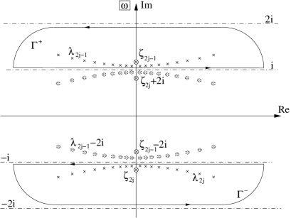
Figure 4: The contours $\Gamma^{\pm}$ only contain Bethe roots $\{\lambda_{k}\}=\{\lambda_{2j}\}\cup\{\lambda_{2j-1}\}$ and the corresponding inhomogeneities $\{\zeta_{k}\}=\{\zeta_{2j}\}\cup\{\zeta_{2j-1}\}$. The Bethe roots and inhomogeneities shifted by the amount of $2{\rm i}$ are located outside.

The combinatorial sum can be converted into a multiple integral by the same token as in equation (65) of [12]. We introduce a function

$$\chi(\lambda,\zeta)={\rm e}(\zeta-\lambda)\mathfrak{a}(\zeta)-{\rm e}(\lambda-\zeta)+\sum_{k=1}^{N}K(\lambda-\lambda_{k})w_{k}(\zeta)\,.$$ (C.16)

Then

$$\mspace{-9.0mu}\chi(\lambda-2{\rm i},\zeta) =\frac{1}{\lambda-\zeta}-\frac{\mathfrak{A}(\zeta)}{\lambda-\zeta-2{\rm i}}+\frac{\mathfrak{a}(\zeta)}{\lambda-\zeta-4{\rm i}}+\sum_{k=1}^{N}\biggl{[}\frac{w_{k}(\zeta)}{\lambda-\lambda_{k}-4{\rm i}}-\frac{w_{k}(\zeta)}{\lambda-\lambda_{k}}\biggr{]}\,,$$ (C.17a)

$$\mspace{-9.0mu}\chi(\lambda+2{\rm i},\zeta) =\frac{\mathfrak{a}(\zeta)}{\lambda-\zeta}-\frac{\mathfrak{A}(\zeta)}{\lambda-\zeta+2{\rm i}}+\frac{1}{\lambda-\zeta+4{\rm i}}+\sum_{k=1}^{N}\biggl{[}\frac{w_{k}(\zeta)}{\lambda-\lambda_{k}}-\frac{w_{k}(\zeta)}{\lambda-\lambda_{k}+4{\rm i}}\biggr{]}.$$ (C.17b)

Let ${\cal R}=\{z\in{\mathbb{C}}|1<|{\rm Im\,}z|<2\}$. Then ${\cal R}$ contains all Bethe roots. The two functions $\chi(\lambda\mp 2{\rm i},\zeta_{j})$ are meromorphic in ${\cal R}$. Their only poles inside ${\cal R}$ are all simple and are located at the Bethe roots and at $\zeta_{j}$. The corresponding residua are

$$\operatorname{res}_{\lambda=\lambda_{k}}\chi(\lambda-2{\rm i},\zeta_{j})=-w_{k}(\zeta_{j})\,,\quad\operatorname{res}_{\lambda=\zeta_{j}}\chi(\lambda-2{\rm i},\zeta_{j})=1\,,$$ (C.18a)

$$\operatorname{res}_{\lambda=\lambda_{k}}\chi(\lambda+2{\rm i},\zeta_{j})=w_{k}(\zeta_{j})\,,\quad\operatorname{res}_{\lambda=\zeta_{j}}\chi(\lambda+2{\rm i},\zeta_{j})=\mathfrak{a}(\zeta_{j})\,.$$ (C.18b)

Define two simple contours $\Gamma^{\pm}$, such that (i) $\Gamma^{+}$ is inside the upper strip of ${\cal R}$ and $\Gamma^{-}$ is inside the lower strip of ${\cal R}$, and (ii) all Bethe roots and all $\zeta_{j}$, $j=1,\dots,2m$, are inside $\Gamma=\Gamma^{+}+\Gamma^{-}$ (see figure 4). Decompose $\Gamma$ in such a way that $\Gamma={\cal B}+{\cal I}$, where $\cal B$ contains only Bethe roots and $\cal I$ contains only inhomogeneity parameters. Then we are very much in the same situation as in [12], and using the functions $\chi(\lambda\pm 2{\rm i},\zeta_{j})$ we can transform the right hand side of (C.14) into a multiple integral over $\Gamma$. As we shall see the notation

$$g_{j}(\omega|\zeta)=\begin{cases}\chi(\omega-2{\rm i},\zeta)&j\leq p\\ \chi(\omega+2{\rm i},\zeta)&j>p\end{cases}$$ (C.19)

will prove useful in that exercise. Using also (C.15) we obtain

$$D^{[2]}(\mathbf{x}|\zeta)\biggl{[}\prod_{j=1}^{m}-2{\rm i}\mathfrak{B}(\xi_{j}-{\rm i})\operatorname{sign}\delta_{j}\biggr{]}\prod_{1\leq j<k\leq m}(\xi_{k}-\xi_{j})^{2}[(\xi_{k}-\xi_{j})^{2}+4]\\ =\lim_{\varepsilon\rightarrow 0+}\sum_{(\{\varepsilon^{+}\},\{\varepsilon^{-}\})\in p_{2}({\mathbb{Z}}_{2m})}\>\biggl{[}\prod_{j=1}^{n}\int_{\cal I}\frac{{\rm d}\omega_{\varepsilon_{j}^{-}}}{2\pi{\rm i}}\biggr{]}\sum_{\ell_{\varepsilon_{1}^{+}},\dots,\ell_{\varepsilon_{2m-n}^{+}}=1}^{N}\quad\sum_{\begin{subarray}{c}(\{\delta^{+}\},\{\delta^{-}\})\in p_{2}({\mathbb{Z}}_{2m})\\ \operatorname{card}\{\delta^{-}\}=n\end{subarray}}\operatorname{sign}(PQ)\\[4.30554pt] \underbrace{\sum_{R\in{\mathfrak{S}}^{n}}\operatorname{sign}(R)\>g_{\varepsilon_{1}^{-}}(\omega_{\varepsilon_{1}^{-}},\zeta_{\delta_{Rj}^{-}})\dots g_{\varepsilon_{n}^{-}}(\omega_{\varepsilon_{n}^{-}},\zeta_{\delta_{Rn}^{-}})}_{\det[g_{\varepsilon_{j}^{-}}(\omega_{\varepsilon_{j}^{-}},\zeta_{\delta_{Rk}^{-}})]}\frac{\det\bigl{[}w_{\ell_{\varepsilon_{j}^{+}}}(\zeta_{\delta_{k}^{+}})\bigr{]}}{\prod_{1\leq j<k\leq 2m}(\omega_{j}-\omega_{k}-2{\rm i})}\biggr{|}_{\omega_{\varepsilon_{j}^{+}}=\lambda_{\ell_{\varepsilon_{j}^{+}}}}\\[4.30554pt] \Biggl{[}\prod_{\begin{subarray}{c}j=1\\ \varepsilon_{j}^{+}\leq p\end{subarray}}^{2m-n}-F^{[1]}_{\varepsilon_{j}^{+}}(\lambda_{\ell_{\varepsilon_{j}^{+}}})\Biggr{]}\Biggl{[}\prod_{\begin{subarray}{c}j=1\\ \varepsilon_{j}^{+}>p\end{subarray}}^{2m-n}\overline{F}^{[1]}_{\varepsilon_{j}^{+}}(\lambda_{\ell_{\varepsilon_{j}^{+}}})\Biggr{]}\Biggl{[}\prod_{\begin{subarray}{c}j=1\\ \varepsilon_{j}^{-}\leq p\end{subarray}}^{n}F^{[1]}_{\varepsilon_{j}^{-}}(\omega_{\varepsilon_{j}^{-}})\Biggr{]}\Biggl{[}\prod_{\begin{subarray}{c}j=1\\ \varepsilon_{j}^{-}>p\end{subarray}}^{n}\overline{F}^{[1]}_{\varepsilon_{j}^{-}}(\omega_{\varepsilon_{j}^{-}})\Biggr{]}\\[4.30554pt] =\lim_{\varepsilon\rightarrow 0+}\underbrace{\sum_{(\{\varepsilon^{+}\},\{\varepsilon^{-}\})\in p_{2}({\mathbb{Z}}_{2m})}\>\biggl{[}\prod_{j=1}^{2m-n}\int_{\cal B}\frac{{\rm d}\omega_{\varepsilon_{j}^{+}}}{2\pi{\rm i}}\biggr{]}\biggl{[}\prod_{j=1}^{n}\int_{\cal I}\frac{{\rm d}\omega_{\varepsilon_{j}^{-}}}{2\pi{\rm i}}\biggr{]}}_{=\prod_{j=1}^{2m}\int_{\Gamma}\frac{{\rm d}\omega_{j}}{2\pi{\rm i}}}\frac{1}{\prod_{1\leq j<k\leq 2m}(\omega_{j}-\omega_{k}-2{\rm i})}\\[4.30554pt] \underbrace{\sum_{\begin{subarray}{c}(\{\delta^{+}\},\{\delta^{-}\})\in p_{2}({\mathbb{Z}}_{2m})\\ \operatorname{card}\{\delta^{-}\}=n\end{subarray}}\operatorname{sign}(PQ)\det[g_{\varepsilon_{j}^{+}}(\omega_{\varepsilon_{j}^{+}},\zeta_{\delta_{Rk}^{+}})]\det[g_{\varepsilon_{j}^{-}}(\omega_{\varepsilon_{j}^{-}},\zeta_{\delta_{Rk}^{-}})]}_{=\det[g_{j}(\omega_{j},\zeta_{k})]}\\[4.30554pt] \Biggl{[}\prod_{\begin{subarray}{c}j=1\\ \varepsilon_{j}^{+}\leq p\end{subarray}}^{2m-n}F^{[1]}_{\varepsilon_{j}^{+}}(\omega_{\varepsilon_{j}^{+}})\Biggr{]}\Biggl{[}\prod_{\begin{subarray}{c}j=1\\ \varepsilon_{j}^{+}>p\end{subarray}}^{2m-n}\overline{F}^{[1]}_{\varepsilon_{j}^{+}}(\omega_{\varepsilon_{j}^{+}})\Biggr{]}\Biggl{[}\prod_{\begin{subarray}{c}j=1\\ \varepsilon_{j}^{-}\leq p\end{subarray}}^{n}F^{[1]}_{\varepsilon_{j}^{-}}(\omega_{\varepsilon_{j}^{-}})\Biggr{]}\Biggl{[}\prod_{\begin{subarray}{c}j=1\\ \varepsilon_{j}^{-}>p\end{subarray}}^{n}\overline{F}^{[1]}_{\varepsilon_{j}^{-}}(\omega_{\varepsilon_{j}^{-}})\Biggr{]}\\[4.30554pt] =\lim_{\varepsilon\rightarrow 0+}\biggl{[}\prod_{j=1}^{p}\int_{\Gamma}\frac{{\rm d}\omega_{j}}{2\pi{\rm i}}F^{[1]}_{j}(\omega_{j})\biggr{]}\biggl{[}\prod_{j=p+1}^{2m}\int_{\Gamma}\frac{{\rm d}\omega_{j}}{2\pi{\rm i}}\overline{F}^{[1]}_{j}(\omega_{j})\biggr{]}\frac{\det[g_{j}(\omega_{j},\zeta_{k})]}{\prod_{1\leq j<k\leq 2m}(\omega_{j}-\omega_{k}-2{\rm i})}\,.$$ (C.20)

Note that we used the Laplace expansion formula for determinants in the third equation.

To summarize up to this point, we have derived the equation

$$D^{[2]}(\mathbf{x}|\zeta)=\lim_{\varepsilon\rightarrow 0+}\prod_{1\leq j<k\leq m}\frac{1}{(\xi_{k}-\xi_{j})^{2}[(\xi_{k}-\xi_{j})^{2}+4]}\\[4.30554pt] \biggl{[}\prod_{j=1}^{p}\int_{\Gamma}\frac{{\rm d}\omega_{j}}{2\pi{\rm i}}F^{[1]}_{j}(\omega_{j})\biggr{]}\biggl{[}\prod_{j=p+1}^{2m}\int_{\Gamma}\frac{{\rm d}\omega_{j}}{2\pi{\rm i}}\overline{F}^{[1]}_{j}(\omega_{j})\biggr{]}\frac{\det[g_{j}(\omega_{j},\zeta_{k})]\prod_{j=1}^{m}\frac{{\rm i}\operatorname{sign}\delta_{j}}{2\mathfrak{B}(\xi_{j}-{\rm i})}}{\prod_{1\leq j<k\leq 2m}(\omega_{j}-\omega_{k}-2{\rm i})}\,.$$ (C.21)

Here the factor $\prod_{j=1}^{m}\operatorname{sign}\delta_{j}$ can be used to reorder the columns in the determinant. Defining the alternating pattern

$$\nu_{2k-1}=\xi_{k}+{\rm i}(1+\varepsilon)\,,\quad\nu_{2k}=\xi_{k}-{\rm i}(1+\varepsilon)$$ (C.22)

and

$$\chi^{(p,\varepsilon)}_{jk}=\begin{cases}\chi(\lambda_{j}-2{\rm i},\nu_{k})&j=1,\dots,p\\[4.30554pt] \chi(\lambda_{j}+2{\rm i},\nu_{k})&j=p+1,\dots,2m\,,\end{cases}$$ (C.23)

we find that

$$\det[g_{j}(\omega_{j},\zeta_{k})]\prod_{j=1}^{m}\operatorname{sign}\delta_{j}=\det\chi^{(p,\varepsilon)}_{jk}\,.$$ (C.24)

Note that the limit $\varepsilon\rightarrow 0+$ is not obvious at this stage, because in the limit the poles of $g$ at the inhomogeneity parameters unavoidably cross the narrow contour $\Gamma$. Below we shall widen the contour, while carefully taking account of the additional terms generated during this process. As we shall see, all additional terms are of order $\varepsilon$ and vanish in the limit.

C.2.2 Fusion of wave functions

Before coming to this point we have to recall that for the spin-1 density matrix elements we do not exactly need $D^{[2]}(\mathbf{x}|\zeta)$, but certain combinations of these coefficients. This leeds to ‘fusion of the wave functions’ $F^{[1]}$, $\overline{F}^{[1]}$, to be described in this subsection.

Let us consider a specific matrix element

$${D^{[2]}}^{\alpha_{1},\dots,\alpha_{m}}_{\beta_{1},\dots,\beta_{m}}(\xi)=\frac{\langle\Psi_{0}|{T^{[2]}}^{\alpha_{1}}_{\beta_{1}}(\xi_{1})\dots T^{[2]}{}^{\alpha_{m}}_{\beta_{m}}(\xi_{m})|\Psi_{0}\rangle}{\langle\Psi_{0}|\Psi_{0}\rangle\Lambda^{[2]}(\xi_{1})\dots\Lambda^{[2]}(\xi_{m})}$$ (C.25)

of the spin-1 density matrix. Since the local space is spin-1, the indices take three different values, $\alpha_{j},\beta_{k}=+,0,-$. The right hand side of (C.25) can be written as a linear combination of coefficients $D^{[2]}(\mathbf{x}|\xi)$ which can be identified by means of (47).

To begin with let us assume that ${T^{[2]}}^{+}_{+}(\xi_{\ell})={T^{[1]}}^{+}_{+}(\xi_{\ell}-{\rm i}){T^{[1]}}^{+}_{+}(\xi_{\ell}+{\rm i})$ is contained in the sequence of monodromy matrix elements on the right hand side of (C.25). Then we must have $x_{j}=2\ell$ and $x_{j+1}=2\ell-1$ for some $j\in\{1,\dots,p-1\}$ in all coefficients $D^{[2]}(\mathbf{x}|\xi)$ contained in the linear combination for that specific density matrix element. Also $\delta_{\ell}=-1-\varepsilon$, and a factor

$$\prod_{k=1}^{2\ell-1} (\omega_{j}-\zeta_{k}-2{\rm i})\prod_{k=2\ell+1}^{2m}(\omega_{j}-\zeta_{k})\prod_{k=1}^{2\ell-2}(\omega_{j+1}-\zeta_{k}-2{\rm i})\prod_{k=2\ell}^{2m}(\omega_{j+1}-\zeta_{k})$$

$$=\bigl{[}(\omega_{j}-\xi_{\ell}-{\rm i})(\omega_{j+1}-\xi_{\ell}-{\rm i})-{\rm i}\varepsilon(\omega_{j}-\omega_{j+1}-2{\rm i})+\varepsilon(2+\varepsilon)\bigr{]}$$

$$\qquad\times\prod_{n=j}^{j+1}\>\prod_{k=1}^{\ell-1}\bigl{[}(\omega_{n}-\xi_{k}-3{\rm i})(\omega_{n}-\xi_{k}-{\rm i})+\varepsilon(2+\varepsilon)\bigr{]}$$

$$\mspace{180.0mu}\times\prod_{k=\ell+1}^{m}\bigl{[}(\omega_{n}-\xi_{k}-{\rm i})(\omega_{n}-\xi_{k}+{\rm i})+\varepsilon(2+\varepsilon)\bigr{]}$$

$$=F_{\ell}(\omega_{j})F_{\ell}(\omega_{j+1})+{\cal O}(\varepsilon)$$ (C.26)

appears. Here we used the ‘spin-1 wave function’ $F_{\ell}$ defined in (65).

In a similar way we may consider all the matrix elements of $T^{[2]}$ using for simplification the right hand side of (47). E.g. if ${T^{[2]}}^{+}_{0}(\xi_{\ell})=\sqrt{2}{T^{[1]}}^{+}_{+}(\xi_{\ell}+{\rm i}){T^{[1]}}^{+}_{-}(\xi_{\ell}-{\rm i})$ is contained in the sequence of monodromy matrix elements on the right hand side of (C.25), then $\delta_{\ell}=1+\varepsilon$, and we have $x_{j}=2\ell$, $x_{j+1}=2\ell-1$ for some $j\in\{1,\dots,p-1\}$ and $x_{i}=2\ell$ for some $i\in\{p+1,\dots,2m\}$. Thus, there is a factor

$$\sqrt{2}\bigl{[}(\omega_{j}-\xi_{\ell}-{\rm i})(\omega_{j+1}-\xi_{\ell}-{\rm i})+{\rm i}(2+\varepsilon)(\omega_{j}-\omega_{j+1}-2{\rm i})+\varepsilon(2+\varepsilon)\bigr{]}$$

$$\qquad\times\prod_{n=j}^{j+1}\>\prod_{k=1}^{\ell-1}\bigl{[}(\omega_{n}-\xi_{k}-3{\rm i})(\omega_{n}-\xi_{k}-{\rm i})+\varepsilon(2+\varepsilon)\bigr{]}$$

$$\mspace{180.0mu}\times\prod_{k=\ell+1}^{m}\bigl{[}(\omega_{n}-\xi_{k}-{\rm i})(\omega_{n}-\xi_{k}+{\rm i})+\varepsilon(2+\varepsilon)\bigr{]}$$

$$\qquad\times(\omega_{i}-\xi_{\ell}+{\rm i}-{\rm i}\varepsilon)\prod_{k=1}^{\ell-1}\bigl{[}(\omega_{i}-\xi_{k}+3{\rm i})(\omega_{i}-\xi_{k}+{\rm i})+\varepsilon(2+\varepsilon)\bigr{]}$$

$$\mspace{180.0mu}\times\prod_{k=\ell+1}^{m}\bigl{[}(\omega_{i}-\xi_{k}-{\rm i})(\omega_{i}-\xi_{k}+{\rm i})+\varepsilon(2+\varepsilon)\bigr{]}$$

$$\equiv\sqrt{2}\,F_{\ell}(\omega_{j})F_{\ell}(\omega_{j+1})\overline{F}_{\ell}(\omega_{i})+{\cal O}(\varepsilon)$$ (C.27)

under the integral. Again $F_{\ell}$ and $\overline{F}_{\ell}$ are taken from (65). We use the notation ‘$\equiv$’ for ‘equal under the multiple integral’ (C.21). The crucial point here is that the term proportional to $(2+\varepsilon)(\omega_{j}-\omega_{j+1}-2{\rm i})$ does not contribute under the integral (C.21) for symmetry considerations. This is because it multiplies a function which is symmetric in $\omega_{j}$ and $\omega_{j+1}$ in (C.2.2) and the only other terms under the integral depending on $\omega_{j}$ and $\omega_{j+1}$ are $\det[g_{j}(\omega_{j},\zeta_{k})]$ and $\prod_{1\leq j<k\leq 2m}(\omega_{j}-\omega_{k}-2{\rm i})$. But

$$\frac{(\omega_{j}-\omega_{j+1}-2{\rm i})\det[g_{j}(\omega_{j},\zeta_{k})]}{\prod_{1\leq j<k\leq 2m}(\omega_{j}-\omega_{k}-2{\rm i})}$$

is antisymmetric in $\omega_{j}$ and $\omega_{j+1}$.

Another example is the matrix element ${T^{[2]}}^{0}_{0}(\xi_{\ell})={T^{[1]}}^{-}_{+}(\xi_{\ell}-{\rm i}){T^{[1]}}^{+}_{-}(\xi_{\ell}+{\rm i})+{T^{[1]}}^{-}_{-}(\xi_{\ell}-{\rm i}){T^{[1]}}^{+}_{+}(\xi_{\ell}+{\rm i})$ for which $\delta_{\ell}=-1-\varepsilon$. It is the only matrix element which we have to express by a sum of two products of monodromy matrix elements with spin-$\frac{1}{2}$ auxiliary space, and it contributes a factor

$$\prod_{k=1}^{2\ell-1} (\omega_{j}-\zeta_{k}-2{\rm i})\prod_{k=2\ell+1}^{2m}(\omega_{j}-\zeta_{k})$$

$$\times\biggl{[}\prod_{k=1}^{2\ell-1}(\omega_{i}-\zeta_{k}+2{\rm i})\prod_{k=2\ell+1}^{2m}(\omega_{i}-\zeta_{k})+\prod_{k=1}^{2\ell-2}(\omega_{i}-\zeta_{k}+2{\rm i})\prod_{k=2\ell}^{2m}(\omega_{i}-\zeta_{k})\biggr{]}$$

$$=2F_{\ell}(\omega_{j})\overline{F}_{\ell}(\omega_{i})+{\cal O}(\varepsilon)\,,$$ (C.28)

where $j\in\{1,\dots,p\}$ and $i\in\{p+1,\dots,2m\}$.

Matrix element	Factor under the integral
${T^{[2]}}^{+}_{+}(\xi_{\ell})$	$F_{\ell}(\omega_{j})F_{\ell}(\omega_{j+1})+{\cal O}(\varepsilon)$
${T^{[2]}}^{+}_{0}(\xi_{\ell})$	$\sqrt{2}\,F_{\ell}(\omega_{j})F_{\ell}(\omega_{j+1})\overline{F}_{\ell}(\omega_{i})+{\cal O}(\varepsilon)$
${T^{[2]}}^{+}_{-}(\xi_{\ell})$	$F_{\ell}(\omega_{j})F_{\ell}(\omega_{j+1})\overline{F}_{\ell}(\omega_{i})\overline{F}_{\ell}(\omega_{i+1})+{\cal O}(\varepsilon)$
${T^{[2]}}^{0}_{+}(\xi_{\ell})$	$\sqrt{2}\,F_{\ell}(\omega_{j})+{\cal O}(\varepsilon)$
${T^{[2]}}^{0}_{0}(\xi_{\ell})$	$2F_{\ell}(\omega_{j})\overline{F}_{\ell}(\omega_{i})+{\cal O}(\varepsilon)$
${T^{[2]}}^{0}_{-}(\xi_{\ell})$	$\sqrt{2}\,F_{\ell}(\omega_{j})\overline{F}_{\ell}(\omega_{i})\overline{F}_{\ell}(\omega_{i+1})+{\cal O}(\varepsilon)$
${T^{[2]}}^{-}_{+}(\xi_{\ell})$	$1$
${T^{[2]}}^{-}_{0}(\xi_{\ell})$	$\sqrt{2}\;\overline{F}_{\ell}(\omega_{i})+{\cal O}(\varepsilon)$
${T^{[2]}}^{-}_{-}(\xi_{\ell})$	$\overline{F}_{\ell}(\omega_{i})\overline{F}_{\ell}(\omega_{i+1})+{\cal O}(\varepsilon)$

Table 1: The polynomials under the integral.

Proceeding case by case in a similar way we obtain the result exposed in tabular 1. In the tabular it is always implied that $j,j+1\in\{1,\dots,p\}$ and $i,i+1\in\{p+1,\dots,2m\}$. Inspecting the tabular we see that, up to corrections of the order of $\varepsilon$, the ‘wave function’ under the integral is composed in the following way: For every zero in the sequences $(\alpha_{j})$ and $(\beta_{k})$ we obtain a factor of $\sqrt{2}$, amounting to a total factor of $2^{(n_{0}(\alpha)+n_{0}(\beta))/2}=2^{m-n_{+}(\alpha)-n_{-}(\beta)}$. For every plus in $(\alpha_{j})$ a factor $F_{\ell}(\omega_{j})F_{\ell}(\omega_{j+1})$ appears and for every zero a factor $F_{\ell}(\omega_{j})$. From the sequence $(\beta_{k})$ we obtain a factor $\overline{F}_{\ell}(\omega_{i})$ for every zero and a factor $\overline{F}_{\ell}(\omega_{i})\overline{F}_{\ell}(\omega_{i+1})$ for every minus sign. This makes a total number of $2n_{+}(\alpha)+n_{0}(\alpha)+n_{0}(\beta)+2n_{-}(\beta)=2m$ factors, and $p=2n_{+}(\alpha)+n_{0}(\alpha)$. With the factors we obtain a sequence $(z_{j})_{j=1}^{2m}$, $z_{j}\in\{1,\dots,m\}$ by arranging them in the order of ascending $\omega_{j}$: $F_{z_{1}}(\omega_{1})\dots F_{z_{p}}(\omega_{p})\overline{F}_{z_{p+1}}\dots\overline{F}_{z_{2m}}(\omega_{2m})$.

Thus, we have obtained the representation

$${D^{[2]}}^{\alpha_{1},\dots,\alpha_{m}}_{\beta_{1},\dots,\beta_{m}}(\xi)=\frac{2^{-n_{+}(\alpha)-n_{-}(\beta)}\prod_{j=1}^{m}\frac{{\rm i}}{\mathfrak{B}(\xi_{j}-{\rm i})}}{\prod_{1\leq j<k\leq m}(\xi_{k}-\xi_{j})^{2}[(\xi_{k}-\xi_{j})^{2}+4]}\\[4.30554pt] \lim_{\varepsilon\rightarrow 0+}\biggl{[}\prod_{j=1}^{2m}\int_{\Gamma}\frac{{\rm d}\omega_{j}}{2\pi{\rm i}}\biggr{]}\frac{\det\chi^{(p,\varepsilon)}_{jk}}{\prod_{1\leq j<k\leq 2m}(\omega_{j}-\omega_{k}-2{\rm i})}\\[4.30554pt] \bigl{[}F_{z_{1}}(\omega_{1})\dots F_{z_{p}}(\omega_{p})\overline{F}_{z_{p+1}}(\omega_{p+1})\dots\overline{F}_{z_{2m}}(\omega_{2m})+{\cal O}(\varepsilon)\bigr{]}$$ (C.29)

for the spin-1 density matrix elements. What remains to do is to calculate the limit $\varepsilon\rightarrow 0$. For this purpose we have to deform the integration contours first.

C.2.3 Widening the contours

Next we would like to show that

$$\biggl{[}\prod_{j=1}^{2m}\int_{\Gamma}\frac{{\rm d}\omega_{j}}{2\pi{\rm i}}\biggr{]}\frac{\det\chi^{(p,\varepsilon)}_{jk}}{\prod_{1\leq j<k\leq 2m}(\omega_{j}-\omega_{k}-2{\rm i})}\\[2.15277pt] \bigl{[}F_{z_{1}}(\omega_{1})\dots F_{z_{p}}(\omega_{p})\overline{F}_{z_{p+1}}(\omega_{p+1})\dots\overline{F}_{z_{2m}}(\omega_{2m})+{\cal O}(\varepsilon)\bigr{]}\\[4.30554pt] \mspace{-120.0mu}=\biggl{[}\prod_{j=1}^{p}\int_{\cal C}\frac{{\rm d}\omega_{j}}{2\pi{\rm i}}\biggr{]}\biggl{[}\prod_{j=p+1}^{2m}\int_{\overline{\cal C}}\frac{{\rm d}\omega_{j}}{2\pi{\rm i}}\biggr{]}\frac{\det\chi^{(p,\varepsilon)}_{jk}}{\prod_{1\leq j<k\leq 2m}(\omega_{j}-\omega_{k}-2{\rm i})}\\[2.15277pt] \bigl{[}F_{z_{1}}(\omega_{1})\dots F_{z_{p}}(\omega_{p})\overline{F}_{z_{p+1}}(\omega_{p+1})\dots\overline{F}_{z_{2m}}(\omega_{2m})+{\cal O}(\varepsilon)\bigr{]}+{\cal O}(\varepsilon)\,.$$ (C.30)

We recall that the simple closed contours $\cal C$, $\overline{\cal C}$ are defined in such a way that

$${\cal C}={\cal C}^{+}+{\cal C}^{-}\,,\quad\overline{\cal C}=\overline{\cal C}^{+}+\overline{\cal C}^{-}$$

$${\cal C}^{\pm}\,,\overline{\cal C}^{\pm}\subset{\cal S}^{\pm}$$

$${\cal C}^{-}=\overline{\cal C}^{-}\,,\quad{\cal C}^{-}\ \text{inside}\ {\cal C}^{+}-2{\rm i}\,,\quad\overline{\cal C}^{+}-2{\rm i}\ \text{inside}\ {\cal C}^{-}$$

$$\Gamma\ \text{inside}\ {\cal C}\,,\overline{\cal C}\,.$$ (C.31)

For ${\cal C}^{\pm}$, $\overline{\cal C}^{\pm}$ we may take large rectangles inside ${\cal S}^{\pm}$ which are slightly narrower than 2 in imaginary direction. The third line in (C.2.3) is a closed contour analogon of the regularization by infinitesimal shifts of the contours in [21]. The Bethe roots of the dominant state come in complex conjugated pairs, so-called 2-strings. For their enumeration we shall employ the same convention as in [21]. Those in the upper half plane will be labeled by odd integers and those in the lower half plane by even integers. By definition the contours ${\cal C}$ and $\overline{\cal C}$ encircle not only all Bethe roots $\lambda_{j}$ and all inhomogeneities $\nu_{j}$ but also the down-shifted upper Bethe roots $\lambda_{2j-1}-2{\rm i}$ and the up-shifted lower Bethe roots $\lambda_{2j}+2{\rm i}$ as well as the down-shifted upper inhomogeneities $\nu_{2j-1}-2{\rm i}$ and the up-shifted lower inhomogeneities $\nu_{2j}+2{\rm i}$.

In preparation of the proof of (C.30) we introduce the notation

$$f(\omega_{1},\dots,\omega_{2m})=\frac{F_{z_{1}}(\omega_{1})\dots F_{z_{p}}(\omega_{p})\overline{F}_{z_{p+1}}(\omega_{p+1})\dots\overline{F}_{z_{2m}}(\omega_{2m})+{\cal O}(\varepsilon)}{\prod_{1\leq j<k\leq 2m}(\omega_{j}-\omega_{k}-2{\rm i})}\,,$$ (C.32)

where the polynomial, including the ${\cal O}(\varepsilon)$ contribution, is the same as under the integrals in (C.30). Then the integral on the right hand side of (C.30) can be written as

$$\sum_{Q\in{\mathfrak{S}}^{2m}}\operatorname{sign}(Q)\int_{{\cal C}}\frac{{\rm d}\omega_{1}}{2\pi{\rm i}}\chi(\omega_{1}-2{\rm i},\nu_{Q1})\dots\int_{{\cal C}}\frac{{\rm d}\omega_{p}}{2\pi{\rm i}}\chi(\omega_{p}-2{\rm i},\nu_{Qp})\\ \int_{\overline{\cal C}}\frac{{\rm d}\omega_{2m}}{2\pi{\rm i}}\chi(\omega_{2m}+2{\rm i},\nu_{Q(2m)})\dots\int_{\overline{\cal C}}\frac{{\rm d}\omega_{p+1}}{2\pi{\rm i}}\chi(\omega_{p+1}+2{\rm i},\nu_{Q(p+1)})\>f(\omega_{1},\dots,\omega_{2m})\,.$$ (C.33)

We shall show that, if we successively replace the integrals in this expression by integrals over $\Gamma$, the total error will be of the order $\varepsilon$.

(a) For the rightmost integral we note that $f$ considered as a function of $\omega_{p+1}$ is holomorphic inside $\overline{\cal C}$. There is a factor $(\omega_{1}-\omega_{p+1}-2{\rm i})\dots(\omega_{p}-\omega_{p+1}-2{\rm i})(\omega_{p+1}-\omega_{p+2}-2{\rm i})\dots(\omega_{p+1}-\omega_{2m}-2{\rm i})$ in the denominator, but with our choice of contours $\omega_{j}-2{\rm i}$ is outside $\overline{\cal C}$ for $\omega_{j}\in{\cal C}$, $j=1,\dots,p$, and the same is true for $\omega_{j}+2{\rm i}$ for $\omega_{j}\in\overline{\cal C}$, $j=p+2,\dots,2m$. The function $\chi(\omega_{p+1}+2{\rm i},\nu_{Q(p+1)})$ has outside $\Gamma$ but inside $\overline{\cal C}$ at most a single pole occurring at $\nu_{Q(p+1)}-2{\rm i}$ if $Q(p+1)$ is odd. Then there is $\ell\in{\mathbb{Z}}_{m}$ such that $\nu_{Q(p+1)}-2{\rm i}=\xi_{\ell}-{\rm i}+{\rm i}\varepsilon$ and, if we contract the contour from $\overline{\cal C}$ to $\Gamma$, the pole contributes a term having a factor $\overline{F}_{z_{p+1}}(\xi_{\ell}-{\rm i}+{\rm i}\varepsilon)={\cal O}(\varepsilon)$ in the numerator. Hence, the numerator of this term is ${\cal O}(\varepsilon)$. In the denominator we have factors of $\omega_{j}-\nu_{Q(p+1)}=\omega_{j}-\xi_{\ell}-{\rm i}-{\rm i}\varepsilon$ for $j=1,\dots,p$ or $\nu_{Q(p+1)}-\omega_{j}-4{\rm i}=\xi_{\ell}-\omega_{j}-3{\rm i}+{\rm i}\varepsilon$ for $j=p+2,\dots,2m$. It follows that the absolute value of the denominator is bounded from below if the $\omega_{j}$ are on ${\cal C}$ for $j=1,\dots,p$ or on $\overline{\cal C}$ for $j=p+2,\dots,2m$. Hence, the additional term that may be generated by contracting the contour from $\overline{\cal C}$ to $\Gamma$ will at most contribute to order $\varepsilon$, even after performing the summation and the remaining integrations in (C.33). We symbolize this by writing

$$\int_{\overline{\cal C}}\frac{{\rm d}\omega_{p+1}}{2\pi{\rm i}}\chi(\omega_{p+1}+2{\rm i},\nu_{Q(p+1)})f(\omega_{1},\dots,\omega_{2m})\equiv_{\varepsilon}\\ \int_{\Gamma}\frac{{\rm d}\omega_{p+1}}{2\pi{\rm i}}\chi(\omega_{p+1}+2{\rm i},\nu_{Q(p+1)})f(\omega_{1},\dots,\omega_{2m})\,.$$ (C.34)

(b) In order to proceed by induction we define

$$I_{0}=f(\omega_{1},\dots,\omega_{2m})\,,$$ (C.35a)

$$I_{n}=\int_{\Gamma}\frac{{\rm d}\omega_{p+n}}{2\pi{\rm i}}\chi(\omega_{p+n}+2{\rm i},\nu_{Q(p+n)})I_{n-1}\,,\quad n=1,\dots,2m-p\,.$$ (C.35b)

We want to show that

$$\int_{\overline{\cal C}}\frac{{\rm d}\omega_{p+n}}{2\pi{\rm i}}\chi(\omega_{p+n}+2{\rm i},\nu_{Q(p+n)})I_{n-1}\equiv_{\varepsilon}I_{n}\,.$$ (C.36)

We have already shown that this is valid for $n=1$. To proceed further we have to know the structure of $I_{n}$.

(c) As a preparatory step let us consider the left hand side (C.36) for $n=2$. Then

$$I_{1}=\sum_{k_{p+1}=1}^{N}f(\omega_{1},\dots,\omega_{p},\lambda_{k_{p+1}},\omega_{p+2},\dots,\omega_{2m})w_{k_{p+1}}(\nu_{Q(p+1)})\\ +f(\omega_{1},\dots,\omega_{p},\nu_{Q(p+1)},\omega_{p+2},\dots,\omega_{2m})\mathfrak{a}(\nu_{Q(p+1)})\,.$$ (C.37)

Here we have used that $f$ is holomorphic as a function of $\omega_{p+1}$ for $\omega_{p+1}$ on and inside $\Gamma$. We insert $I_{1}$ into the left hand side of (C.36) for $n=2$ and contract the integration contour from $\overline{\cal C}$ to $\Gamma$. Due to our special choice of the contours ${\cal C}$, $\overline{\cal C}$ the poles at $\omega_{p+2}=\omega_{j}-2{\rm i}$, $j=1,\dots,p$ and at $\omega_{p+2}=\omega_{j}+2{\rm i}$, $j=p+3,\dots,2m$, remain outside the contour during the process of deformation. The only pole of $\chi(\omega_{p+2}+2{\rm i},\nu_{Q(p+2)})$ which may be crossed is, in case that $Q(p+2)$ is odd, a simple pole at $\nu_{Q(p+2)}-2{\rm i}$. The situation is the same as in case (a) above. And as above we can see that such a term gives only an order-$\varepsilon$ contribution, even after performing the sum and the remaining integrals: $\nu_{Q(p+2)}=\xi_{\ell}+{\rm i}+{\rm i}\varepsilon\ \Rightarrow\ \overline{F}_{z_{p+2}}(\nu_{Q(p+2)}-2{\rm i})={\cal O}(\varepsilon)$ and in the denominator we may have $\omega_{j}-\nu_{Q(p+2)}=\omega_{j}-\xi_{\ell}-{\rm i}-{\rm i}\varepsilon$ for $j=1,\dots,p$ or $\nu_{Q(p+2)}-\omega_{j}-4{\rm i}=\xi_{\ell}-\omega_{j}-3{\rm i}+{\rm i}\varepsilon$ for $j=p+3,\dots,2m$, as before, or $\lambda_{k_{p+1}}-\nu_{Q(p+2)}$ or $\nu_{Q(p+1)}-\nu_{Q(p+2)}$. The latter terms are of no danger, since we assume that the $\xi_{j}$ are mutually distinct and distinct from all Bethe roots. Thus, we see that the same argument as above works.

However, we now have singularities of $I_{1}$ which are crossed in the course of the deformation of the contour. They give additional contributions. The summand with $k_{p+1}=j$ has a term $\lambda_{j}-\omega_{p+2}-2{\rm i}$ in the denominator, giving rise to a simple pole in $\omega_{p+2}$ at $\lambda_{j}-2{\rm i}$, if $j$ is odd. When contracting the contour of the $\omega_{p+2}$-integral this pole causes a contribution (see (C.16), (C.8)) proportional to

$$\chi(\lambda_{j},\nu_{Q(p+2)})w_{j}(\nu_{Q(p+1)})=\mathfrak{a}^{\prime}(\lambda_{j})w_{j}(\nu_{Q(p+2)})w_{j}(\nu_{Q(p+1)})$$ (C.38)

which is symmetric in $p+1$, $p+2$. Such a term vanishes under the sum over all permutations in (C.33). Another additional contribution comes from the second term in (C.37), which has a factor $\nu_{Q(p+1)}-\omega_{p+2}-2{\rm i}$ in the denominator. So we have a pole at $\nu_{Q(p+1)}-2{\rm i}$. It will give only ${\cal O}(\varepsilon)$-corrections when we integrate over $\omega_{p+2}$, as we have already seen.

(d) In the general case the argument is very similar. $I_{n-1}$ is obtained by iterating the integrations over $\Gamma$. In every integration the $I_{j-1}$ under the integral is holomorphic on and inside $\Gamma$ by construction. Hence, we obtain a sum over the pole contributions of $\chi(\omega_{p+j}+2{\rm i},\nu_{Q(p+j)})$. This means that $I_{n-1}$ is a sum over terms of the form

$$t(\omega_{p+n})=f(\omega_{1},\dots,\omega_{p},x_{p+1},\dots,x_{p+n-1},\omega_{p+n},\dots,\omega_{2m})\>y_{p+1}\dots y_{p+n-1}\,,$$ (C.39)

where $x_{j}$ is either a Bethe root or $\nu_{Qj}$. If $x_{j}$ is a Bethe root, say $\lambda_{\ell}$, then the corresponding factor $y_{j}=w_{\ell}(\nu_{Qj})$, if $x_{j}=\nu_{Qj}$, then $y_{j}=\mathfrak{a}(\nu_{Qj})$. Let us consider

$$\int_{\overline{\cal C}}\frac{{\rm d}\omega_{p+n}}{2\pi{\rm i}}\chi(\omega_{p+n}+2{\rm i},\nu_{Q(p+n)})t(\omega_{p+n})\,.$$ (C.40)

If we shrink the contour to $\Gamma$, we obtain at most one pole contribution from $\chi$ which is at $\nu_{Q(p+n)}-2{\rm i}$ if $Q(p+n)$ is odd. This contribution is ${\cal O}(\varepsilon)$ by the same argument as above. Also for the contributions stemming from $t$ we can argue as above. Note that we do not have to consider double poles (or poles of even higher order), since, if $x_{j}$ and $x_{k}$ are the same Bethe root, $\lambda_{\ell}$ say, then $t(\omega_{p+n})$ has a factor $w_{\ell}(\nu_{Qj})w_{\ell}(\nu_{Qk})$, which vanishes under the antisymmetrizing sum in (C.33). Thus, we have accomplished the proof of (C.36).

(e) It follows from (C.36) that we can replace all the $\overline{\cal C}$-integrals in (C.33) by $\Gamma$-integrals. The total error will be only of order $\varepsilon$. To finish the proof of (C.30) we have to proceed with the contours ${\cal C}$. Let us set

$$J_{p+1}=I_{2m-p}\,,$$ (C.41a)

$$J_{n}=\int_{\Gamma}\frac{{\rm d}\omega_{n}}{2\pi{\rm i}}\chi(\omega_{n}-2{\rm i},\nu_{Qn})J_{n+1}\,,\quad n=p,\dots,1\,.$$ (C.41b)

We want to show that

$$\int_{{\cal C}}\frac{{\rm d}\omega_{n}}{2\pi{\rm i}}\chi(\omega_{n}-2{\rm i},\nu_{Qn})J_{n+1}\equiv_{\varepsilon}J_{n}\,.$$ (C.42)

The proof is very similar as before.

(f) Let us start with $n=p$. Then $J_{p+1}=I_{2m-p}$ is a sum over terms of the form

$$s(\omega_{p})=f(\omega_{1},\dots,\omega_{p},x_{p+1},\dots,x_{2m})y_{p+1}\dots y_{2m}\,,$$ (C.43)

as follows from (C.39). If we shrink the contour in

$$\int_{{\cal C}}\frac{{\rm d}\omega_{p}}{2\pi{\rm i}}\chi(\omega_{p}-2{\rm i},\nu_{Qp})s(\omega_{p})$$ (C.44)

to $\Gamma$, we obtain at most a single pole contribution from $\chi$ stemming from a pole at $\nu_{Qp}+2{\rm i}$ in case that $Qp$ is even. Then $\nu_{Qp}+2{\rm i}=\xi_{\ell}+{\rm i}-{\rm i}\varepsilon$ for some $\ell\in{\mathbb{Z}}_{m}$. But now $F_{z_{p}}(\xi_{\ell}+{\rm i}-{\rm i}\varepsilon)={\cal O}(\varepsilon)$, and the numerator in the generated term is ${\cal O}(\varepsilon)$. The denominator contains terms $\omega_{j}-(\nu_{Qp}+2{\rm i})-2{\rm i}=\omega_{j}-\xi_{\ell}-3{\rm i}+{\rm i}\varepsilon$ which are bounded from below in the absolute value for $\omega_{j}\in{\cal C}$, $j=1,\dots,p-1$. Hence, the whole term is of order $\varepsilon$, even after integration and summation, and can safely be forgotten. As for the singularities of $s(\omega_{p})$ we have again two types. If $x_{j}$ is a Bethe root, say $\lambda_{\ell}$, then a term $\omega_{p}-\lambda_{\ell}-2{\rm i}$ occurs in the denominator. It comes together with a factor $w_{\ell}(\nu_{Qj})$. When calculating the residue at $\lambda_{\ell}+2{\rm i}$, which is non-zero only if $\ell$ is even, we obtain something proportional to

$$\chi(\lambda_{\ell},\nu_{Qp})w_{\ell}(\nu_{Qj})=\mathfrak{a}^{\prime}(\lambda_{\ell})w_{\ell}(\nu_{Qp})w_{\ell}(\nu_{Qj})$$ (C.45)

which yields a term that vanishes under the sum in (C.33) due to symmetry reasons. Double poles can be excluded by the same argument as above. Finally we may have $x_{j}=\nu_{Qj}$. Then a factor $\omega_{p}-\nu_{Qj}-2{\rm i}$ is present in the denominator resulting again at most in an ${\cal O}(\varepsilon)$-contribution.

(g) Iterating the above arguments we obtain (C.42), and the proof of (C.30) is complete. With (C.30) we can now perform the limit $\varepsilon\rightarrow 0+$, because it is trivial at the right hand side of the equation. With the definition

$$\chi^{(p)}_{jk}=\lim_{\varepsilon\rightarrow 0+}\chi^{(p,\varepsilon)}_{jk}$$ (C.46)

we obtain

$$\lim_{\varepsilon\rightarrow 0+}\biggl{[}\prod_{j=1}^{2m}\int_{\Gamma}\frac{{\rm d}\omega_{j}}{2\pi{\rm i}}\biggr{]}\frac{\det\chi^{(p,\varepsilon)}_{jk}}{\prod_{1\leq j<k\leq 2m}(\omega_{j}-\omega_{k}-2{\rm i})}\\[2.15277pt] \bigl{[}F_{z_{1}}(\omega_{1})\dots F_{z_{p}}(\omega_{p})\overline{F}_{z_{p+1}}(\omega_{p+1})\dots\overline{F}_{z_{2m}}(\omega_{2m})+{\cal O}(\varepsilon)\bigr{]}\\[4.30554pt] \mspace{-120.0mu}=\biggl{[}\prod_{j=1}^{p}\int_{\cal C}\frac{{\rm d}\omega_{j}}{2\pi{\rm i}}F_{z_{j}}(\omega_{j})\biggr{]}\biggl{[}\prod_{j=p+1}^{2m}\int_{\overline{\cal C}}\frac{{\rm d}\omega_{j}}{2\pi{\rm i}}\overline{F}_{z_{j}}(\omega_{j})\biggr{]}\frac{\det\chi^{(p)}_{jk}}{\prod_{1\leq j<k\leq 2m}(\omega_{j}-\omega_{k}-2{\rm i})}\,.$$ (C.47)

With this we have derived the multiple integral representation

$${D^{[2]}}^{\alpha_{1},\dots,\alpha_{m}}_{\beta_{1},\dots,\beta_{m}}(\xi)=\frac{2^{-n_{+}(\alpha)-n_{-}(\beta)}}{\prod_{1\leq j<k\leq m}(\xi_{k}-\xi_{j})^{2}[(\xi_{k}-\xi_{j})^{2}+4]}\\[4.30554pt] \biggl{[}\prod_{j=1}^{p}\int_{\cal C}\frac{{\rm d}\omega_{j}}{2\pi{\rm i}}F_{z_{j}}(\omega_{j})\biggr{]}\biggl{[}\prod_{j=p+1}^{2m}\int_{\overline{\cal C}}\frac{{\rm d}\omega_{j}}{2\pi{\rm i}}\overline{F}_{z_{j}}(\omega_{j})\biggr{]}\frac{\det\chi^{(p)}_{jk}\>\prod_{j=1}^{m}\frac{{\rm i}}{\mathfrak{B}(\xi_{j}-{\rm i})}}{\prod_{1\leq j<k\leq 2m}(\omega_{j}-\omega_{k}-2{\rm i})}$$ (C.48)

for the inhomogeneous density matrix of the isotropic spin-1 chain.

C.3 The linear integral equations

In this subsection we shall derive a pair of coupled integral equations for the functions $\chi(\lambda\pm 2{\rm i},\nu)$. For this purpose we first of all note that the function $\chi$ has been defined in (C.16) in such a way that

$$\chi(\lambda_{j},\nu)=\mathfrak{a}^{\prime}(\lambda_{j})w_{j}(\nu)\,,\quad j=1,\dots,N$$ (C.49)

(see (C.8)). We shall use some of the functions that appear in the formulation of the thermodynamics of the model [30] and that are collected in appendix 7. In first place we need the functions $\mathfrak{A}$ and $\overline{\mathfrak{A}}$ (see (A.7a)). It follows from their definition and from the fact that $\Lambda^{[1]}$ has no zeros in ${\cal S}^{+}\cup{\cal S}^{-}$ that the only zeros of $\mathfrak{A}(\lambda+2{\rm i})$ in ${\cal S}^{-}$ are simple zeros at $\lambda_{2j-1}-2{\rm i}$, while the only poles in ${\cal S}^{-}$ are simple poles at $\lambda_{2j}$. Similarly, the only zeros of $\overline{\mathfrak{A}}(\lambda-2{\rm i})$ in ${\cal S}^{+}$ are simple zeros at $\lambda_{2j}+2{\rm i}$ and its only poles in ${\cal S}^{+}$ are simple and located at $\lambda_{2j-1}$.

Hence, using (C.17b), (C.49), we conclude that the only singularities of the function $\chi(\lambda+2{\rm i},\xi^{+})/\mathfrak{A}(\lambda+2{\rm i})$ inside ${\cal S}^{-}$ are

1. a simple pole at $\lambda=\xi^{-}$ with residue $-1$,

2. simple poles at $\lambda=\lambda_{2k-1}-2{\rm i}$ with residua $w_{2k-1}(\xi^{+})$.

Similarly, all singularities of $\chi(\lambda-2{\rm i},\xi^{+})/\overline{\mathfrak{A}}(\lambda-2{\rm i})$ inside ${\cal S}^{+}$ are (see (C.17a) and (C.49))

1. a simple pole at $\lambda=\xi^{+}$ with residue $1/\overline{\mathfrak{A}}(\xi^{-})$,

2. simple poles at $\lambda=\lambda_{2k}+2{\rm i}$ with residua $-w_{2k}(\xi^{+})$.

With this it follows by means of (C.17) that

$$\chi(\lambda-2{\rm i},\xi^{+})=\frac{\mathfrak{A}(\xi^{+})}{\lambda-\xi^{+}-4{\rm i}}-\frac{\mathfrak{B}(\xi^{-})}{\mathfrak{A}(\xi^{-})}\frac{1}{\lambda-\xi^{+}-2{\rm i}}-\frac{\mathfrak{a}(\xi^{-})}{\mathfrak{A}(\xi^{-})}\frac{1}{\lambda-\xi^{-}}$$

$$\mspace{18.0mu}-\int_{{\cal C}^{+}}\frac{{\rm d}\mu}{2\pi{\rm i}}\frac{\chi(\mu-2{\rm i},\xi^{+})}{\overline{\mathfrak{A}}(\mu-2{\rm i})}K(\lambda-\mu)+\int_{\overline{\cal C}^{-}}\frac{{\rm d}\mu}{2\pi{\rm i}}\frac{\chi(\mu+2{\rm i},\xi^{+})}{\mathfrak{A}(\mu+2{\rm i})}K(\lambda-\mu-4{\rm i})\,,$$ (C.50a)

$$\chi(\lambda+2{\rm i},\xi^{+})=\frac{\mathfrak{A}(\xi^{+})}{\lambda-\xi^{+}}-\frac{\mathfrak{B}(\xi^{-})}{\mathfrak{A}(\xi^{-})}\frac{1}{\lambda-\xi^{-}}-\frac{\mathfrak{a}(\xi^{-})}{\mathfrak{A}(\xi^{-})}\frac{1}{\lambda-\xi^{-}+4{\rm i}}$$

$$\mspace{18.0mu}-\int_{\overline{\cal C}^{+}}\frac{{\rm d}\mu}{2\pi{\rm i}}\frac{\chi(\mu-2{\rm i},\xi^{+})}{\overline{\mathfrak{A}}(\mu-2{\rm i})}K(\lambda-\mu+4{\rm i})+\int_{{\cal C}^{-}}\frac{{\rm d}\mu}{2\pi{\rm i}}\frac{\chi(\mu+2{\rm i},\xi^{+})}{\mathfrak{A}(\mu+2{\rm i})}K(\lambda-\mu)$$ (C.50b)

for $\lambda\in{\cal C}^{+}$ in the first equation and $\lambda\in{\cal C}^{-}$ in the second equation.

If now $\nu=\xi^{-}$ we have to repeat almost the same considerations. The function $\chi(\lambda+2{\rm i},\xi^{-})/\mathfrak{A}(\lambda+2{\rm i})$ has the following singularities inside ${\cal S}^{-}$:

1. an simple pole at $\lambda=\xi^{-}$ with residue $\mathfrak{a}(\xi^{-})/\mathfrak{A}(\xi^{+})$,

2. simple poles at $\lambda=\lambda_{2k-1}-2{\rm i}$ with residues $w_{2k-1}(\xi^{-})$.

Furthermore, all singularities of $\chi(\lambda-2{\rm i},\xi^{-})/\overline{\mathfrak{A}}(\lambda-2{\rm i})$ inside ${\cal S}^{+}$ are

1. a simple pole at $\xi^{+}$ with residue $-\mathfrak{a}(\xi^{-})$,

2. simple poles at $\lambda=\lambda_{2k}+2{\rm i}$ with residua $-w_{2k}(\xi^{-})$.

Thus, we obtain

$$\chi(\lambda-2{\rm i},\xi^{-})=-\frac{\mathfrak{a}(\xi^{-})}{\mathfrak{A}(\xi^{+})}\frac{1}{\lambda-\xi^{+}-4{\rm i}}-\frac{\mathfrak{B}(\xi^{-})}{\mathfrak{A}(\xi^{+})}\frac{1}{\lambda-\xi^{+}}+\frac{\mathfrak{A}(\xi^{-})}{\lambda-\xi^{-}}$$

$$\mspace{18.0mu}-\int_{{\cal C}^{+}}\frac{{\rm d}\mu}{2\pi{\rm i}}\frac{\chi(\mu-2{\rm i},\xi^{-})}{\overline{\mathfrak{A}}(\mu-2{\rm i})}K(\lambda-\mu)+\int_{\overline{\cal C}^{-}}\frac{{\rm d}\mu}{2\pi{\rm i}}\frac{\chi(\mu+2{\rm i},\xi^{-})}{\mathfrak{A}(\mu+2{\rm i})}K(\lambda-\mu-4{\rm i})\,,$$ (C.51a)

$$\chi(\lambda+2{\rm i},\xi^{-})=-\frac{\mathfrak{a}(\xi^{-})}{\mathfrak{A}(\xi^{+})}\frac{1}{\lambda-\xi^{+}}-\frac{\mathfrak{B}(\xi^{-})}{\mathfrak{A}(\xi^{+})}\frac{1}{\lambda-\xi^{-}+2{\rm i}}+\frac{\mathfrak{A}(\xi^{-})}{\lambda-\xi^{-}+4{\rm i}}$$

$$\mspace{18.0mu}-\int_{\overline{\cal C}^{+}}\frac{{\rm d}\mu}{2\pi{\rm i}}\frac{\chi(\mu-2{\rm i},\xi^{-})}{\overline{\mathfrak{A}}(\mu-2{\rm i})}K(\lambda-\mu+4{\rm i})+\int_{{\cal C}^{-}}\frac{{\rm d}\mu}{2\pi{\rm i}}\frac{\chi(\mu+2{\rm i},\xi^{-})}{\mathfrak{A}(\mu+2{\rm i})}K(\lambda-\mu)\,,$$ (C.51b)

where $\lambda\in{\cal C}^{+}$ in the first equation and $\lambda\in{\cal C}^{-}$ in the second equation.

After taking the Trotter limit $N\rightarrow\infty$ the driving terms in the integral equations above are singular at $\xi=0$. The singularity can be removed by taking appropriate linear combinations. We define

$$\begin{pmatrix}G^{\pm}(\lambda,\xi)\\ S^{\pm}(\lambda,\xi)\end{pmatrix}=\begin{pmatrix}\mathfrak{A}(\xi^{-})/\mathfrak{B}(\xi^{-})&\mathfrak{A}(\xi^{+})/\mathfrak{B}(\xi^{-})\\ -1/\mathfrak{A}(\xi^{+})&1/\mathfrak{A}(\xi^{-})\end{pmatrix}\begin{pmatrix}\chi(\lambda\mp 2{\rm i},\xi^{+})\\ \chi(\lambda\mp 2{\rm i},\xi^{-})\end{pmatrix}\,.$$ (C.52)

Then, using also (A.9a)-(A.9c), we arrive at equations (66), (67) of the main body of the text.

In order to express the determinant under the integral in (C.48) in terms of the functions $G^{\pm}$, $S^{\pm}$ we use the matrix $\Theta^{(p)}$ defined in (69). Because the determinant of the matrix in (C.52) is $2/\mathfrak{B}(\xi^{-})$, we obtain

$$\det\Theta_{j,k}^{(p)}=\biggl{[}\prod_{j=1}^{m}\frac{2{\rm i}}{\mathfrak{B}(\xi_{j}-{\rm i})}\biggr{]}\det\chi_{jk}^{(p)}\,.$$ (C.53)

Inserting this into (C.48) we arrive at the multiple integral representation (70).

References

[1]
H. M. Babujian, Exact solution of the one-dimensional isotropic
Heisenberg chain with arbitrary spins S, Phys. Lett. A 90
(1982) 479.
[2]
H. Boos and F. Göhmann, On the physical part of the factorized
correlation functions of the XXZ chain, J. Phys. A 42 (2009)
315001.
[3]
H. Boos, F. Göhmann, A. Klümper and J. Suzuki, Factorization of
multiple integrals representing the density matrix of a finite segment of the
Heisenberg spin chain, J. Stat. Mech. (2006) P04001.
[4]
—, Factorization of the finite temperature correlation functions of the
XXZ chain in a magnetic field, J. Phys. A 40 (2007) 10699.
[5]
H. Boos, M. Jimbo, T. Miwa, F. Smirnov and Y. Takeyama, Hidden
Grassmann structure in the XXZ model, Comm. Math. Phys. 272
(2007) 263.
[6]
—, Hidden Grassmann structure in the XXZ model II: creation
operators, Comm. Math. Phys. 286 (2009) 875.
[7]
H. E. Boos and V. E. Korepin, Quantum spin chains and Riemann zeta
function with odd arguments, J. Phys. A 34 (2001) 5311.
[8]
A. H. Bougourzi and R. A. Weston, N-point correlation functions of the
spin-1 XXZ model, Nucl. Phys. B 417 (1994) 439.
[9]
J. Damerau, F. Göhmann, N. P. Hasenclever and A. Klümper, Density
matrices for finite segments of Heisenberg chains of arbitrary length, J.
Phys. A 40 (2007) 4439.
[10]
T. Deguchi and C. Matsui, Correlation functions of the integrable
higher-spin XXX and XXZ spin chains through the fusion method, Nucl.
Phys. B 831 (2010) 359.
[11]
F. H. L. Essler, H. Frahm, F. Göhmann, A. Klümper and V. E. Korepin,
The One-Dimensional Hubbard Model (Cambridge University Press,
2005).
[12]
F. Göhmann, N. P. Hasenclever and A. Seel, The finite temperature
density matrix and two-point correlations in the antiferromagnetic XXZ
chain, J. Stat. Mech. (2005) P10015.
[13]
F. Göhmann, A. Klümper and A. Seel, Integral representations for
correlation functions of the XXZ chain at finite temperature, J. Phys. A
37 (2004) 7625.
[14]
—, Integral representation of the density matrix of the XXZ chain at
finite temperature, J. Phys. A 38 (2005) 1833.
[15]
F. Göhmann and J. Suzuki, Quantum spin chains at finite temperature,
preprint, arXiv:1002.3194 (2010). Contributed to the Festschrift volume in
honour of the 60th birthday of Prof. T. Miwa.
[16]
M. Idzumi, Level-2 irreducible representations of U(q)(sl(2)), vertex
operators, and their correlations, Int. J. Mod. Phys. A 9 (1994)
4449.
[17]
M. Jimbo, K. Miki, T. Miwa and A. Nakayashiki, Correlation functions of
the XXZ model for , Phys. Lett. A 168 (1992) 256.
[18]
M. Jimbo and T. Miwa, Quantum KZ equation with and
correlation functions of the XXZ model in the gapless regime, J. Phys. A
29 (1996) 2923.
[19]
M. Jimbo, T. Miwa and F. Smirnov, Hidden Grassmann structure in the
XXZ model III: introducing Matsubara direction, J. Phys. A 42
(2009) 304018.
[20]
—, On one-point functions of descendants in Sine-Gordon model,
preprint, arXiv:0912.0934 (2009).
[21]
N. Kitanine, Correlation functions of the higher spin XXX chains, J.
Phys. A 34 (2001) 8151.
[22]
N. Kitanine, K. Kozlowski, J. M. Maillet, N. A. Slavnov and V. Terras, On
correlation functions of integrable models associated with the six-vertex
-matrix, J. Stat. Mech. (2007) P01022.
[23]
—, Algebraic Bethe ansatz approach to the asymptotic behavior of
correlation functions, J. Stat. Mech. (2009) P04003.
[24]
N. Kitanine, J. M. Maillet and V. Terras, Correlation functions of the
XXZ Heisenberg spin- chain in a magnetic field, Nucl. Phys.
B 567 (2000) 554.
[25]
A. Klümper, Thermodynamics of the anisotropic spin-1/2 Heisenberg
chain and related quantum chains, Z. Phys. B 91 (1993) 507.
[26]
P. P. Kulish, N. Yu. Reshetikhin and E. K. Sklyanin, Yang-Baxter
equation and representation theory: I, Lett. Math. Phys. 5 (1981)
393.
[27]
P. P. Kulish and E. K. Sklyanin, Quantum spectral transform method –
recent developments, in Lecture Notes in Physics 151, 61–119
(Springer Verlag, Berlin, 1982).
[28]
A. Seel, T. Bhattacharyya, F. Göhmann and A. Klümper, A note on the
spin-1/2 XXZ chain concerning its relation to the Bose gas, J. Stat.
Mech. (2007) P08030.
[29]
A. Seel, F. Göhmann and A. Klümper, From multiple integrals to
Fredholm determinants, Prog. Theor. Phys. Suppl. 176 (2008) 375.
[30]
J. Suzuki, Spinons in magnetic chains of arbitrary spins at finite
temperatures, J. Phys. A 32 (1999) 2341.
[31]
M. Suzuki, Transfer-matrix method and Monte Carlo simulation in quantum
spin systems, Phys. Rev. B 31 (1985) 2957.
[32]
M. Suzuki and M. Inoue, The ST-transformation approach to analytic
solutions of quantum systems. I. General formulations and basic limit
theorems, Prog. Theor. Phys. 78 (1987) 787.
[33]
L. A. Takhtajan, The picture of low-lying excitations in the isotropic
Heisenberg chain of arbitrary spins, Phys. Lett. A 87 (1982) 479.
[34]
A. B. Zamolodchikov and A. V. Fateev, A model factorized -matrix and
an integrable spin- Heisenberg chain, Yad. Fiz. 32 (1980) 581.