Fractional Boltzmann equation for resonance radiation transport in plasma

Abstract

The fractional Boltzmann equation for resonance radiation transport in plasma is proposed. We start from the standard Boltzmann equation, averaging over frequencies leads to appearance of fractional derivative. This fact is in accordance with the conception of latent variables leading to hereditary and non-local dynamics (in particular, fractional dynamics). The presence of the fractional material derivative in the equation is concordant with heavy tailed distribution of photon path lengths and with spatiotemporal coupling peculiar to the process. We discuss some methods of solution of the obtained equation and demonstrate numerical results in some simple cases.

,

1 Introduction

The standard (Markovian) transport model based on the Boltzmann equation can not describe some non-equilibrium processes called anomalous that take place in turbulent plasma, interstellar magnetic fields, disordered semiconductors, and other complex structures (see Bouchaud & Georges (1990); Metzler & Klafter (2000)). Causes of anomality lie in non-uniformly scaled (fractal) spatial heterogeneities, in which particle trajectories take cluster form. Furthermore, particles can be located in some domains of small sizes (traps) for a long time. Estimations show that path length and waiting time distributions are often characterized by heavy tails of the power law type. This behavior allows to introduce time and space derivatives of fractional orders. Distinction of path length distribution from exponential is interpreted as a consequence of media fractality, and analogous property of waiting time distribution as a presence of memory.

During last decades, essential progress in description of the asymptotical behavior of such processes is achieved by passage from the standard diffusion equations to the equations with fractional derivatives (see, for example, Metzler & Klafter (2000), Samko et al. (1993), Hilfer (2000), Podlubny (1999), West et al. (2002), Nigmatullin (2006), Sibatov & Uchaikin (2009), Uchaikin et al. (2008), Datsko & Gafiychuk (2010)). The diffusion equation describes only asymptotical part of the solution of the Boltzmann equation. For more complete description the passage to fractional derivatives should be performed not from the diffusion equation but on the previous stage, i. e. from the Boltzmann equation.

Nonnenmacher & Nonnenmacher (1989) proposed fractional generalization of the bilinear Boltzmann equation in the form

$$\frac{\partial f(\mathbf{r},\mathbf{v},t)}{\partial t}=\ _{0}\textsf{D}^{1-\nu}_{t}\left[\frac{}{}\textsf{C}(f,f)+S(\mathbf{r},\mathbf{v},t)\right.$$

$$\left.-\mathbf{v}\frac{\partial f(\mathbf{r},\mathbf{v},t)}{\partial\mathbf{r}}-\frac{\mathbf{F}}{m}\frac{\partial f(\mathbf{r},\mathbf{v},t)}{\partial\mathbf{v}}\right],$$ (1)

where $f(\mathbf{r},\mathbf{v},t)$ is the one-particle distribution function, $\textsf{C}(f,f)$ is the collision integral, and ${}_{0}\textsf{D}^{1-\nu}_{t}$ is the Riemann-Liouville partial derivative of fractional order $1-\nu$, $0<\nu<1$. The derivation of this equation stated in Nonnenmacher & Nonnenmacher (1989) is rather formal. It is based on the analogy between corresponding standard diffusion equation and its fractional generalization. Nevertheless, it leads to valid asymptotic equations whose solutions are consistent with Monte Carlo simulation. However, one should clearly understand what the equation describes. Authors Nonnenmacher & Nonnenmacher (1989) have not paid sufficient attention to this issue. The fractional equation describes hereditary kinetics with memory kernel of power law type which is usually caused by waiting times in local domains with power law asymptotes in distribution function. The process does not assume spatial-temporal coupling: the waiting times are considered to be independent of random free path lengths distributed according to exponential law. Moreover, the detailed consideration concerned only one-dimensional process.

The linear Boltzmann equation describing the anomalous transport of neutrons within processes of scattering, fission, and absorption, was generalized to fractional form by Kadem & Baleanu (2010) and its solution was considered under more realistic conditions.

We are going to consider fractional generalized kinetics in connection with radiation transport in plasmas. The standard Boltzmann equation has found very important applications in studying transport of particles in plasma. It is known (see Pereira et al. (2004), Berberan-Santos et al. (2006), Pereira et al. (2007)) that a stochastic behavior of atomic resonance radiation migration in plasma is of superdiffusive type. Pereira et al. (2004) have shown that photon trajectories for Doppler, Lorentz, and Voight line shapes under the assumption about complete frequency redistribution are Lévy flights. Superdiffusivity is a consequence of the heavy-tailed nature of path length distribution

$$P(\xi)=\mathrm{Prob}\{R>\xi\}\propto\xi^{-\nu}.$$

The lighter the tail of the line shape function, the less heavy the tail of path length pdf. Berberan-Santos et al. (2006) concluded that this tail is always heavy ($\nu\leq 1$).

Finiteness of photon velocities assumes that the process is Lévy walks, not Lévy flights. Lévy walks give a proper dynamical description of the superdiffusive behavior. The temporal and spatial variables of Lévy walks are strongly correlated. Zolotarev et al. (1999), Zaburdaev & Chukbar (2002), Sokolov & Metzler (2003), Chukbar & Zaburdaev (2003), Uchaikin & Sibatov (2004), Uchaikin & Sibatov (2009)) proposed equations for Lévy walks, but these equations are obtained in diffusion approximation and authors concentrate on the one-dimensional case.

In the present paper, we derive the fractional Boltzmann equation for propagation of resonance radiation in plasma. We start from the standard Boltzmann equation, which suppose exponential distribution of path lengths of photon with a given frequency $\omega$. Averaging over the random frequency leads to power law distribution of path length (see Pereira et al. (2004)) and to appearance of fractional derivative in the equation. This fact is in accordance with the conception of latent variables leading to fractional dynamics (see Uchaikin (2008)). It is interesting that equation contains three-dimensional material derivative generalizing the one-dimensional case introduced in Sokolov & Metzler (2003). Finally, we discuss methods of solution of the obtained equation and present results in some simple cases.

2 Peculiarities of the process

The process under consideration looks as follows. Initial photon with frequency $\omega^{\prime}$ and velocity $c$ entering the gas goes a random free path $R$ distributed according to the exponential law

$$\mathrm{Prob}\{R>\xi|\omega\}=\exp(-\sigma(\omega)\xi).$$

Then, it interacts with an atom which absorbs the photon passing to excitement state. After a random time $T$, the atom re-radiates a photon with a frequency $\omega$ being close to the initial $\omega$ but not coinciding with them. The irradiated photon continues its way as before.

Therefore, the first special feature of the process is a finite speed of light. The second one is the random delay of the photon re-emission. And the third, most important feature of resonance excitation transport in a spectrum line is the fact that frequency dependence of absorption factor $\sigma(\omega)$ repeats a shape of the very radiation spectral line $w(\omega)$. This leads to a specific situation: most of irradiated photons have very short free paths and they are absorbed again, practically at once, so that only small fraction of photons having frequencies in tails of spectrum (far from the center of the line) can go far from re-emission points. We observe L$\grave{e}$vy walk.

The resonance radiation transport theory develops in two directions – in light-engineering and in astrophysics. In the first of them, the finiteness of speed of light is neglected, that is, one accepts $c=\infty$. The main equation in this case is the Biberman-Holstein equation. The second direction concerns astrophysical scales, so that the traveling times are much larger then the excitation times and the latter can be neglected. Here we concentrate our attention on this last problem.

3 Integral transport equation

For the sake of convenience, they usually identify radiated and absorbed photons, in other words, they say that an atom absorbing a photon radiates ”the same photon” with frequency and direction changed after an interaction with the atom, or shorter, the photon is scattered on the atom. This process is described by the linear Boltzmann equation

$$\left(\frac{\partial}{\partial t}+c\mathbf{\Omega}\nabla\right)\Phi(\mathbf{r},\mathbf{\Omega},\omega,t)+c\sigma(\omega)\Phi(\mathbf{r},\mathbf{\Omega},\omega,t)$$

$$=\int\int d\mathbf{\Omega}^{\prime}d\omega^{\prime}w(\omega\leftarrow\omega^{\prime})W(\mathbf{\Omega}\leftarrow\mathbf{\Omega}^{\prime})c\sigma(\omega^{\prime})\Phi(\mathbf{r},\mathbf{\Omega}^{\prime},\omega^{\prime},t)$$

$$+\Phi_{0}(\mathbf{r},\mathbf{\Omega},\omega)\frac{}{}\delta(t),$$ (2)

which can be transformed to a pure integral form:

$$\Phi(\mathbf{r},\mathbf{\Omega},\omega,t)=\Phi_{0}(\mathbf{r},\mathbf{\Omega},\omega,t)$$

$$+\int\limits_{0}^{\infty}d\xi\ e^{-\sigma(\omega)\xi}\int\int d\mathbf{\Omega}^{\prime}d\omega^{\prime}\ w(\omega\leftarrow\omega^{\prime})W(\mathbf{\Omega}\leftarrow\mathbf{\Omega}^{\prime})$$

$$\times\sigma(\omega^{\prime})\Phi(\mathbf{r}-\mathbf{\Omega}\ \xi,\mathbf{\Omega^{\prime}},\omega^{\prime},t-\xi/c).$$

Here $\Phi(\mathbf{r},\mathbf{\Omega},\omega,t)d\mathbf{r}d\mathbf{\Omega}d\omega$ is the mean number of photons at the moment $t$ in volume $d\mathbf{r}=dxdydz$ flying into solid angle $d\mathbf{\Omega}$ with frequencies in $[\omega,\omega+d\omega)$ Further, we use the standard assumptions.

• Assumption 1. The complete frequency redistribution takes place:

  $$w(\omega\leftarrow\omega^{\prime})=w(\omega)$$

• Assumption 2. The local thermodynamic equilibrium is valid:

  $$\sigma(\omega)=Cw(\omega)$$

Passing to the photon collision density

$$F(\mathbf{r},\mathbf{\Omega},\omega,t)\equiv c\sigma(\omega)\Phi(\mathbf{r},\mathbf{\Omega},\omega,t),$$

we arrive at

$$F(\mathbf{r},\mathbf{\Omega},\omega,t)=F_{0}(\mathbf{r},\mathbf{\Omega},\omega,t)+$$

$$+\int\limits_{0}^{\infty}d\xi\ w(\omega)\sigma(\omega)e^{-\sigma(\omega)\xi}\int d\mathbf{\Omega}^{\prime}\int d\omega^{\prime}\ W(\mathbf{\Omega}\leftarrow\mathbf{\Omega}^{\prime})\times$$

$$\times F(\mathbf{r}-\mathbf{\Omega}\ \xi,\mathbf{\Omega^{\prime}},\omega^{\prime},t-\xi/c)$$

Integrating over frequency

$$F(\mathbf{r},\mathbf{\Omega},t)=\int\limits_{0}^{\infty}F(\mathbf{r},\mathbf{\Omega},\omega,t)d\omega,$$

we obtain the following integral equation

$$F(\mathbf{r},\mathbf{\Omega},t)-F_{0}(\mathbf{r},\mathbf{\Omega},t)=$$

$$=\int\limits_{0}^{\infty}d\xi\ p(\xi)\int d\mathbf{\Omega}^{\prime}W(\mathbf{\Omega}\leftarrow\mathbf{\Omega}^{\prime})\ F(\mathbf{r}-\mathbf{\Omega}\ \xi,\mathbf{\Omega^{\prime}},t-\xi/c),$$

where the kernel is given by

$$p(\xi)=\left\langle\sigma(\omega)e^{-\sigma(\omega)\xi}\right\rangle=\int\limits_{0}^{\infty}w(\omega)\sigma(\omega)e^{-\sigma(\omega)\xi}d\omega.$$

Characteristic feature of resonance radiation propagation is the fact that absorption spectrum (as an approximation of thermodynamic equilibrium and total redistribution of frequency) is proportional to the spectrum of radiation

$$\sigma(\omega)=Cw(\omega)$$

Calculations lead us to the following asymptotic properties of the path length distribution

$$P(\xi)=\left\langle e^{-\sigma(\omega)\xi}\right\rangle\sim\frac{\xi^{-\nu}}{\gamma\Gamma(1-\nu)},$$

$$p(\xi)=-P^{\prime}(\xi)=\left\langle\sigma e^{-\sigma(\omega)\xi}\right\rangle\sim\frac{\xi^{-\nu-1}}{\gamma\Gamma(1-\nu)}.$$

To satisfy this condition, we choose the distribution in the form of ”fractional exponents”:

$$p(\xi)=\gamma\xi^{\nu-1}E_{\nu,\nu}(-\gamma\xi^{\nu}),$$ (3)

where $E_{\alpha,\beta}(x)$ is the two-parameter Mittag-Leffler function (see, for example Uchaikin et al. (2008)).

4 Fractional Boltzmann equation

Generalized Boltzmann equation for the case of path length distribution (3) is obtained in the form

$$\left(\frac{\partial}{\partial t}+c\mathbf{\Omega}\nabla\right)^{\nu}\Phi(\mathbf{r},\mathbf{\Omega},t)+\mu\Phi(\mathbf{r},\mathbf{\Omega},t)=$$

$$=\mu\int W(\mathbf{\Omega}\leftarrow\mathbf{\Omega}^{\prime})\Phi(\mathbf{r},\mathbf{\Omega}^{\prime},t)d\mathbf{\Omega}^{\prime}+$$

$$+\left(\frac{\partial}{\partial t}+c\mathbf{\Omega}\nabla\right)^{\nu-1}\left[\Phi_{0}(\mathbf{r},\mathbf{\Omega})\frac{}{}\delta(t)\right],$$ (4)

where $\mu=c\gamma$ and the operator

$$\left(\frac{\partial}{\partial t}+c\mathbf{\Omega}\nabla\right)^{\nu}\Phi(\mathbf{r},\mathbf{\Omega},t)=$$

$$=\frac{1}{\Gamma(1-\nu)}\left(\frac{\partial}{\partial t}+c\mathbf{\Omega}\nabla\right)\int\limits_{0}^{t}\frac{\Phi(\mathbf{r}-c\mathbf{\Omega}(t-\tau),\mathbf{\Omega},\tau)}{(t-\tau)^{\nu}}d\tau$$ (5)

is the fractional generalization of the material derivative.

Ordinary material derivative is determined as

$$\left(\frac{\partial}{\partial t}+\mathbf{c}\frac{\partial}{\partial\mathbf{r}}\right)f(\mathbf{r},t)=\lim\limits_{h\downarrow 0}\frac{f(\mathbf{r},t)-f(\mathbf{r}-\mathbf{c}h,t-h)}{h}.$$

The operator

$$A=-\left(\frac{\partial}{\partial t}+\mathbf{c}\frac{\partial}{\partial\mathbf{r}}\right)$$

is the infinitesimal operator generating the semigroup of operators

$$T_{h}f(\mathbf{r},t)=f(\mathbf{r}-\mathbf{c}h,t-h)$$

Consequently, we have for $(-A)^{\alpha}$

$$(-A)^{\alpha}f(\mathbf{r},t)=\left(\frac{\partial}{\partial t}+\mathbf{c}\frac{\partial}{\partial\mathbf{r}}\right)^{\alpha}f(\mathbf{r},t)=$$

$$=\lim\limits_{h\downarrow 0}\ \frac{\alpha}{\Gamma(1-\alpha)}\int\limits_{h}^{\infty}s^{-\alpha-1}\left[f(\mathbf{r},t)-f(\mathbf{r}-\mathbf{c}s,t-s)\frac{}{}\right]ds$$

By integrating by parts, the last operator can be reduced to the form

$$\left(\frac{\partial}{\partial t}+\mathbf{c}\frac{\partial}{\partial\mathbf{r}}\right)^{\alpha}f(\mathbf{r},t)=$$

$$=\frac{1}{\Gamma(1-\alpha)}\left(\frac{\partial}{\partial t}+\mathbf{c}\frac{\partial}{\partial\mathbf{r}}\right)\int\limits_{-\infty}^{t}\frac{f(\mathbf{r}-\mathbf{c}(t-\tau),\tau)}{(t-\tau)^{\alpha}}d\tau$$

If we consider the case of a space-homogeneous distribution of particles $\Phi(\mathbf{r},\mathbf{\Omega},t)\equiv\Phi(\mathbf{\Omega},t)$ this operator becomes the fractional Rieman-Liouville derivative of order $\nu$

$$\left(\frac{\partial}{\partial t}+c\mathbf{\Omega}\nabla\right)^{\nu}\Phi(\mathbf{r},\mathbf{\Omega},t)\mapsto\ _{0}\textsf{D}^{\nu}_{t}\Phi(\mathbf{\Omega},t).$$

In a stationary problem, when the function $\Phi(\mathbf{r},\mathbf{\Omega})$ does not depend on time,

$$\left(\frac{\partial}{\partial t}+c\mathbf{\Omega}\nabla\right)^{\nu}\Phi(\mathbf{r},\mathbf{\Omega})\mapsto\ c(\mathbf{\Omega}\nabla)^{\nu}\Phi(\mathbf{r},\mathbf{\Omega},t),$$

this operator represents fractional generalization of the directional derivative.

5 Solutions of fractional Boltzmann equation

5.1 Analytical results

In one-dimensional case, when photons can fly only along of $x$-axis, the fractional generalization of the Boltzmann equation is of the form

$$\left(\frac{\partial}{\partial t}+c\Omega_{x}\frac{\partial}{\partial x}\right)^{\nu}\Phi(x,\Omega_{x},t)+\mu\Phi(x,\Omega_{x},t)=$$

$$=\mu J(x,\Omega_{x},t)+\left(\frac{\partial}{\partial t}+c\Omega_{x}\frac{\partial}{\partial x}\right)^{\nu-1}S(x,\Omega_{x},t).$$

Using expressions for the collision integral

$$J(x,\Omega_{x},t)=\frac{1}{2}\left[\Phi_{+}(x,t)+\Phi_{-}(x,t)\right]\ [\delta(\Omega_{x}-1)+\delta(\Omega_{x}+1)]$$

and for the one-dimensionally ”isotropic” instantaneous source

$$S(x,\Omega_{x},t)=\frac{1}{2}\ [\delta(\Omega_{x}-1)+\delta(\Omega_{x}+1)]\delta(x)\delta(t)$$

we obtain the following equations:

$$\left(\frac{\partial}{\partial t}+c\frac{\partial}{\partial x}\right)^{\nu}\Phi_{+}(x,t)=$$

$$=\frac{\mu}{2}[\Phi_{-}(x,t)-\Phi_{+}(x,t)]+\frac{t^{-\nu}}{2\Gamma(1-\nu)}\ \delta(x-ct)$$

$$\left(\frac{\partial}{\partial t}-c\frac{\partial}{\partial x}\right)^{\nu}\Phi_{-}(x,t)=$$

$$=\frac{\mu}{2}[\Phi_{+}(x,t)-\Phi_{-}(x,t)]+\frac{t^{-\nu}}{2\Gamma(1-\nu)}\ \delta(x+ct)$$

$$\Phi(x,t)=\Phi_{+}(x,t)+\Phi_{-}(x,t)$$

From last equations one follows

$$\left[\left(\frac{\partial}{\partial t}-c\frac{\partial}{\partial x}\right)^{\nu}+\left(\frac{\partial}{\partial t}+c\frac{\partial}{\partial x}\right)^{\nu}+\frac{2}{\mu}\left(\frac{\partial^{2}}{\partial t^{2}}-c^{2}\frac{\partial^{2}}{\partial x^{2}}\right)^{\nu}\right]\Phi(x,t)=$$

$$=\frac{t^{-\nu}}{2\Gamma(1-\nu)}\ [\delta(x-ct)+\delta(x+ct)]-$$

$$-\frac{\nu\ t}{\mu\ [\Gamma(1-\nu)]^{2}}\left(\frac{c^{2}t^{2}-x^{2}}{4c^{2}}\right)^{-1-\nu}.$$ (6)

In the asymptotics of large times the last equation passes into the following one

$$\left[\left(\frac{\partial}{\partial t}-c\frac{\partial}{\partial x}\right)^{\nu}+\left(\frac{\partial}{\partial t}+c\frac{\partial}{\partial x}\right)^{\nu}\right]\Phi(x,t)=$$

$$=\frac{t^{-\nu}}{2\Gamma(1-\nu)}\ [\delta(x-ct)+\delta(x+ct)],$$

solution of which is expressed in terms of elementary functions (see Uchaikin & Sibatov (2009))

$$\Phi(x,t)=\frac{2\sin\pi\nu}{\pi}\times$$

$$\times\frac{\left(1-x^{2}/c^{2}t^{2}\right)^{\nu-1}}{(1-x/ct)^{2\nu}+(1+x/ct)^{2\nu}+2\left(1-x^{2}/c^{2}t^{2}\right)^{\nu}\cos\pi\nu}.$$

Quantitative analysis of distributions can be performed using the method of moments. Due to finiteness of photon velocity, its position is bounded random variable and according to Cramer’s criterion distribution of excitations is unambiguously determined by the moments of this distribution. Moments can be found from a characteristic function.

For the one-dimensional case, the Fourier-Laplace transformation of the equation (6) leads to the following expression

$$\widetilde{\Phi}(k,\lambda)=\frac{(\lambda-ick)^{\nu-1}+(\lambda+ick)^{\nu-1}+\displaystyle\frac{2\lambda}{\mu}\left(\lambda^{2}+c^{2}k^{2}\right)^{\nu}}{(\lambda-ick)^{\nu}+(\lambda+ick)^{\nu}+\displaystyle\frac{2\lambda}{\mu}\left(\lambda^{2}+c^{2}k^{2}\right)^{\nu}}.$$

In the asymptotics of small $k$ and $\lambda$ corresponding to the diffusion limit, we obtain

$$\widetilde{\Phi}(k,\lambda)\sim\frac{(\lambda-ick)^{\nu-1}+(\lambda+ick)^{\nu-1}}{(\lambda-ick)^{\nu}+(\lambda+ick)^{\nu}}.$$

Moments are determined by the relation

$$\tilde{m}_{n}(\lambda)=(-i)^{n}\frac{\partial^{n}\Phi(k,\lambda)}{\partial k^{n}}.$$

In isotropic case, Fourier-Laplace transformation of (4) leads to the following asymptotical form for $\widetilde{\Phi}(\mathbf{k},t)$

$$\widetilde{\Phi}(\mathbf{k},t)\sim\frac{\int\left(\lambda-ic\mathbf{\Omega}\hskip 1.42262pt\mathbf{k}\right)^{\nu-1}d\mathbf{\Omega}}{\int\left(\lambda-ic\mathbf{\Omega}\hskip 1.42262pt\mathbf{k}\right)^{\nu}d\mathbf{\Omega}}.$$

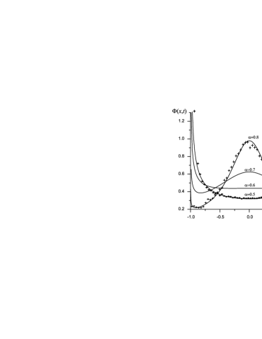
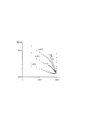
5.2 Numerical results

Here, a computational algorithm for the process is described, realized in the Monte Carlo code and used for computing the resonance radiation and excitation distribution in plasma. An important advantage of the method is simplicity of taking into account boundary conditions and inhomogeneity of the medium.

This method represents randomized scheme of realization of generation expansion. It can be considered as statistical simulation of transport process characterized by known distributions of independent random parameters determining a random trajectory. Set of large number of independent trajectories allows to estimate statistically a process quality interesting for us.

Figure 1: Comparison of analytical solutions with the results of Monte Carlo simulation for isotropically one-dimensional case as functions of dimensionless variable $x/ct$.

Figure 2: Results of Monte Carlo simulation for isotropic 3D case.

There is the typical sequence of operations for simulation of photon trajectory.

–

A position of excited atom at the initial time moment is chosen. PDF of its radius-vector $\mathbf{R}_{0}$ is determined by given initial distribution of excitations $N(\mathbf{r},0)$ through the relation ${p_{\mathbf{R}}=N(\mathbf{r},0)/\int N(\mathbf{r},0)d\mathbf{r}}$.

–

The random time till the moment of photon emission by the atom is generated according to the exponential distribution $p_{T}(t)=\gamma e^{-\gamma t}$.

–

The frequency of emitted photon is distributed with the pdf $w(\omega)$.

–

A direction $\mathbf{\Omega}$ of photon emission is generated. This direction is characterized by random variables $\cos\Theta$ and $\Psi$, which are uniformly distributed (in isotropic case) in $[-1,1]$ and $[0,2\pi)$, respectively.

–

A photon path length $R$ is simulated in infinite homogeneous medium, $p_{R}(\xi)=\sigma(\omega)e^{-\sigma(\omega)\xi}$. If the whole segment $[\mathbf{R}_{0},\mathbf{R}_{0}+\mathbf{\Omega}R]$ keeps within the volume occupied by plasma, its second end is taken as the position of another excited atom. This atom absorbs the photon. If this segment traverses absorbing or transparent boundary, the trajectory comes to the end.

–

For new excited atom, waiting time till the moment of photon emission is simulated. And so on, described operations are repeated before the end of trajectory.

From physical point of view, the fractional operator in the Boltzmann equation means that anomalously long free paths arising from time to time tear the trajectory into more or less localised clusters which look separated at any scale.

Solutions obtained by Monte Carlo simulations are presented in Fig. 1, 2 (points). One-dimensional solutions listed in the previous subsection agree with the numerical results.

6 Conclusion

The fractional generalization of the Boltzmann equation taking into account spatiotemporal coupling peculiar to resonance radiation transport is proposed. This coupling is provided by heavy tailed distribution of photon path lengths which arises after averaging over frequencies and by finiteness of photon velocity. Heavy tails of path length distribution leads to appearance of fractional derivative in the kinetic equation, but due to coupling, this fractional operator represents not simple fractional Laplacian. It is a fractional analogue of the material derivative that is agree with results obtained by Sokolov & Metzler (2003) for one-dimensional Lévy walks.

References

- Pereira et al. (2007) Alves-Pereira, A. R., Nunes-Pereira, E. J., Martinho, J. M. G., Berberan-Santos, M. N. (2007). Photonic superdiffusive motion in resonance radiation trapping. Partial frequency redistribution effects. Journal of Chemical Physics, 126, 154505.
- Berberan-Santos et al. (2006) Berberan-Santos, M. N., Nunes-Pereira, E. J., Martinho, J. M. G. (2006). Photonic superdiffusive motion in resonance radiation trapping. Journal of Chemical Physics, 125, 174308.
- Bouchaud & Georges (1990) Bouchaud, J. P., Georges, A. (1990). Anomalous diffusion in disordered media: statistical mechanisms, models and physical applications. Physics Reports, 195, 127–293.
- Chukbar & Zaburdaev (2003) Chukbar, K. V., Zaburdaev, V. Yu. (2003). Comment on ”Towards deterministic equations for Lévy walks: The fractional material derivative”. Physical Review E, 68, 033101.
- Datsko & Gafiychuk (2010) Datsko, B. Y., Gafiychuk, V. V. (2010). Mathematical modeling of fractional reaction-diffusion systems with different order time derivatives. Journal of Mathematical Sciences, 165, 392–402.
- Hilfer (2000) Hilfer, R. (2000). Applications of Fractional Calculus in Phisics. World Scientific.
- Kadem & Baleanu (2010) Kadem, A., Baleanu, D. (2010). Fractional radiative transfer equation within Chebyshev spectral approach. Computers & Mathematics with Applications, 59, 1865–1873.
- Metzler & Klafter (2000) Metzler, R., Klafter, J. (2000). The random walk’s guide to anomalous diffusion: a fractional dynamics approach. Physics Reports, 339, 1–77.
- Molisch & Oehry (1998) Molisch, A. F., Oehry, B. P. (1998). Radiation Trapping in Atomic Vapours. Clarendon Press, Oxford.
- Nigmatullin (2006) Nigmatullin, R. R. (2006). The realization of the generalized transfer equation in a medium with fractal geometry. Physica Status Solidi (b), 133, 425–430.
- Nonnenmacher & Nonnenmacher (1989) Nonnenmacher, T. F., Nonnenmacher, D. J. F. (1989). Towards the formulation of a nonlinear fractional extended irreversible thermodynamics. Acta Physica Hungarica, 66, 145–154.
- Pereira et al. (2004) Pereira, E., Martinho, J. M. G., Berberan-Santos, M. N. (2004). Photon trajectories in incoherent atomic radiation trapping as Lévy flights. Physical Review Letters, 93, 120201.
- Podlubny (1999) Podlubny, I. (1999). Fractional Differential Equations. Academic Press.
- Samko et al. (1993) Samko, S. G., Kilbas, A. A., Marichev, O. I. (1993). Fractional Integrals and Derivatives – Theory and Application. Gordon and Breach, New York.
- Sibatov & Uchaikin (2009) Sibatov, R. T., Uchaikin, V. V. (2009). Fractional differential approach to dispersive transport in semiconductors. Physics Uspekhi, 52, 1019–1043.
- Sokolov & Metzler (2003) Sokolov, I. M., Metzler, R. (2003). Towards deterministic equations for Lévy walks: The fractional material derivative. Physical Review E, 67, 010101 (R).
- Uchaikin & Zolotarev (1999) Uchaikin, V. V., Zolotarev, V. M. (1999). Chance and Stability, Stable Distributions and their Applications. VSP, Utrecht, The Netherlands.
- Uchaikin & Sibatov (2004) Uchaikin, V. V., Sibatov, R. T. (2004). One-dimensional fractal walk at a finite free motion velocity. Technical Physics Letters, 30, 316- 318.
- Uchaikin et al. (2008) Uchaikin, V. V., Cahoy, D. O., Sibatov, R. T. (2008). Fractional processes: from Poisson to branching one. International Journal of Bifurcation and Chaos, 18, 2717–2725.
- Uchaikin (2008) Uchaikin, V. V. (2008). Method of Fractional Derivatives. Artishok, Ulyanovsk (in Russian).
- Uchaikin & Sibatov (2009) Uchaikin, V. V., Sibatov, R. T. (2009). Statistical model of fluorescence blinking. Journal of Experimental and Theoretical Physics, 109, 537- 546.
- West et al. (2002) West, B. J., Bologna, M., Grigolini, P. (2002). Physics of Fractal Operators. Springer-Verlag, New York.
- Zaburdaev & Chukbar (2002) Zaburdaev, V. Yu., Chukbar, K. V. (2002). Accelerated superdiffusion and finite velocity of Lévy walks. Journal of Experimental and Theoretical Physics, 121, 299–307.
- Zolotarev et al. (1999) Zolotarev, V. M., Uchaikin, V. V., Saenko, V. V. (1999). Superdiffusion and stable laws. Journal of Experimental and Theoretical Physics, 88, 780–787.