Complexes and exactness of certain Artin groups.

Abstract.

In his work on the Novikov conjecture, Yu introduced Property $A$ as a readily verified criterion implying coarse embeddability. Studied subsequently as a property in its own right, Property $A$ for a discrete group is known to be equivalent to exactness of the reduced group $C^{*}$-algebra and to the amenability of the action of the group on its Stone-Cech compactification. In this paper we study exactness for groups acting on a finite dimensional $\operatorname{CAT}(0)$ cube complex. We apply our methods to show that Artin groups of type FC are exact. While many discrete groups are known to be exact the question of whether every Artin group is exact remains open.

1. Introduction

A discrete metric space $X$ has Property $A$ if there exists a sequence of families of finitely supported probability measures $f_{n,x}\in\ell^{1}(X)$, indexed by $x\in X$, and a sequence of constants $S_{n}>0$, such that:

• For every $n$ and $x$ the function $f_{n,x}$ is supported in $B_{S_{n}}(x)$.

• For every $R>0$, we have

  $$\left\|f_{n,x}-f_{n,x^{\prime}}\right\|\to 0$$

  uniformly on the set $\{(x,x^{\prime}):d(x,x^{\prime})\leq R\}$ as $n\to\infty$.

A discrete group has Property $A$ if its underlying proper metric space does (this is independent of the choice of proper metric). In this case the definition is recognized as a non-equivariant form of the Reiter condition for amenability.

For groups it transpires that Property $A$ is equivalent to a wide variety of other conditions including exactness of the reduced group $C^{*}$-algebra, $C^{*}$-exactness of the group itself (defined in terms of crossed products) and amenability of the action of the group on its Stone-Cech compactification [11, 14]. The class of groups possessing Property $A$ is large and diverse – for example, it contains every amenable group, every linear group and every hyperbolic group, and is closed under many natural operations [10, 12, 8]. In this article we shall for groups use the terms Property $A$ and exactness interchangeably.

In previous work, in collaboration with J. Brodzki, S. Campbell and N. Wright, we showed that a finite dimensional $\operatorname{CAT}(0)$ cube complex has Property $A$ [3]. For the proof we constructed an explicit family of weight functions which, when suitably normalised, become the functions $f_{n,x}$ in the definition above. As a consequence a group acting (metrically) properly on a finite dimensional $\operatorname{CAT}(0)$ cube complex is exact. In particular all finitely generated right-angled Artin groups are exact. Since an infinitely generated Artin group is the ascending union of its finitely generated parabolic subgroups any countable right angled Artin group is exact.

In this paper we carry out an extended study of the weight functions, as defined on a suitable compact space combinatorially defined in terms of the hyperplanes and half spaces of the complex. Our analysis of their topological and measure theoretic properties leads to a new inheritance property for exact groups. Indeed, while true that a group acting on a locally finite Property $A$ space with exact stabilisers is exact, the analogous statement for general non-locally finite spaces is false. In order to guarantee inheritence in the more general context one needs to assert control over coarse stabilisers – point stabilisers are not sufficient. In our setting, following an idea of Ozawa [14], extension of the weight functions to a compact space affords the required additional control. We obtain the following result:

Theorem A.

A countable discrete group acting on a finite dimensional $\operatorname{CAT}(0)$ cube complex is exact if and only if each vertex stabilizer of the action is exact.

As an application, we offer the following result in which we do not assume the Artin group is finitely generated.

Theorem B.

An Artin group of type FC is exact.

We note that Altobelli characterised the Artin groups of type FC as the smallest class of Artin groups containing the Artin groups of finite type which is closed under amalgamations along parabolic subgroups [1]. Thus, this theorem could alternately be obtained by appealing to the stability theorem for graph products of exact groups first established in [9]. (See also [8] for a more modern discussion.) However the class of groups acting on $\operatorname{CAT}(0)$ cube complexes is considerably richer than the class of groups acting on trees and we expect Theorem A to have many other applications.

The paper is organised as follows. In Section 2 we recall the definition and basic properties of a $\operatorname{CAT}(0)$ cube complex, with an emphasis on the combinatorics of vertices, hyperplanes and half spaces. We describe a compact space in which the vertex set of the complex embeds, and give an explicit description of the points of this space. In Section 3 we recall the definition of the weight functions from [3] and analyse their topological and measure theoretic properties. In Section 4, adapting slightly the method of Ozawa [14], we establish Theorem A. Section 5 contains relevant background on Artin groups, and a discussion of Theorem B.

2. Cubical complexes

A $\operatorname{CAT}(0)$ cube complex is a cell complex in which each cell is a Euclidean cube of side length $1$ and the attaching maps are isometries; the complex is equipped in the usual way with a geodesic metric which is required to satisfy the $\operatorname{CAT}(0)$ condition of non-positive curvature. It follows that a $\operatorname{CAT}(0)$ cube complex is simply connected, even contractible, as a topological space.

The midpoint of each edge of a $\operatorname{CAT}(0)$ cube complex defines a hyperplane – the union of all geodesics passing through the midpoint at right angles to the underlying edge, the angle being measured in the local Euclidean metric on each cube. Each hyperplane is a totally geodesic codimension one subspace which is locally separating, and therefore globally separating since the complex is simply connected.

In this paper we shall be concerned exclusively with the combinatorics of the vertices, hyperplanes and half spaces of a $\operatorname{CAT}(0)$ cube complex. We shall now outline the facts we require – we refer to [6], and the standard references [2, 15] for additional details.

Let $X$ be a $\operatorname{CAT}(0)$ cube complex. Slightly abusing notation, we shall denote the set of vertices of the complex by $X$ as well. Each hyperplane decomposes the vertex set into two subsets, the two half spaces determined by the hyperplane. There is a priori no reason to prefer one of these half spaces over the other and we shall adopt the following convention: fix a base vertex, and for each hyperplane $H$ denote by $H^{+}$ the half space containing the base vertex; the complementary half space is denoted $H^{-}$. A hyperplane $H$ separates two vertices if one belongs to $H^{+}$ and the other to $H^{-}$.

Let $x$ and $y$ be vertices in $X$. The interval between $x$ and $y$ is the intersection of the half spaces containing both $x$ and $y$; it is a finite set which we shall denote $[x,y]$. It follows directly from the definition that a vertex belongs to $[x,y]$ exactly when there are no hyperplanes which separate it from both $x$ and $y$. A useful alternate description of the interval is the following: $[x,y]$ consists of those vertices in $X$ which lie on an edge geodesic joining $x$ and $y$. Observe that $[x,x]=\{\,x\,\}$. Given three vertices $x,y,z$ the intersection $[x,y]\cap[y,z]\cap[z,x]$ is comprised of a single vertex; we denote this vertex by $m(x,y,z)$ and refer to it as the median of $x$, $y$, $z$.

Let now $\mathcal{H}$ denote the set of hyperplanes in $X$. Each vertex $x$ determines a function $\mathcal{H}\to\{\,\pm 1\,\}$ according to the rule

$$x(H)=\begin{cases}+1,&x\in H^{+}\\ -1,&x\in H^{-}.\end{cases}$$

Observe that $x(H)=-1$ precisely when $H$ separates $x$ and the fixed base vertex. While the notation appears clumsy, it is chosen for convenience in the following statement: for every vertex $x$ and hyperplane $H$ we see that $x$ belongs to the half space $H^{x(H)}$. (Here, we are implicitly writing $H^{+1}$ for $H^{+}$, and similarly for $H^{-}$.) We denote by $\{\,\pm 1\,\}^{\mathcal{H}}$ the Hamming cube on $\mathcal{H}$, that is, the set of functions $\mathcal{H}\to\{\,\pm 1\,\}$ equipped with the infinite product topology. We obtain by the above a map

$$X\to\{\,\pm 1\,\}^{\mathcal{H}}\,.$$

Any two (distinct) vertices are separated by at least one hyperplane and if $H$ separates $x$ and $y$ then $x(H)\neq y(H)$. Thus, this map is injective. We identify $X$ with its image, the subset of original vertices.

An element $z$ of the Hamming cube is an admissible vertex if for every two hyperplanes $H$ and $K$ there exists an original vertex $x$ for which both $x(H)=z(H)$ and $x(K)=z(K)$. Equivalently, $z$ is admissible if for every $H$ and $K$ the half spaces $H^{z(H)}$ and $K^{z(K)}$ have non-empty intersection. Clearly, an original vertex is admissible. Admissible vertices that are not original vertices are ideal vertices.

We pause briefly to consider an example.

Example.

The Euclidean plane equipped with its usual integer lattice squaring is a $\operatorname{CAT}(0)$ cube complex of dimension two. The vertices are the integer lattice points. The hyperplanes are the horizontal and vertical lines intersecting the axes at half-integer points:

$$H_{n}\quad \colon\quad y=n+\tfrac{1}{2}$$

$$K_{n}\quad \colon\quad x=n+\tfrac{1}{2},$$

for an integer $n$. Fix $(0,0)$ as the base vertex.

The lattice point $(p,q)$ in the first quadrant defines an original vertex by

$$(p,q)(H_{n})=\begin{cases}-1,&\text{when $0\leq n<q$}\\ +1,&\text{else},\end{cases}\qquad(p,q)(K_{n})=\begin{cases}-1,&\text{when $0\leq n<p$}\\ +1,&\text{else}.\end{cases}$$

There are also ideal vertices. For example, we may orient all horizontal lines to point upwards and all vertical lines to point to the right defining an admissable vertex $(+\infty,+\infty)$ by

$$(+\infty,+\infty)(H_{n})=\begin{cases}+1,&\text{when $n<0$}\\ -1,&\text{else},\end{cases}\qquad(+\infty,+\infty)(K_{n})=\begin{cases}+1,&\text{when $n<0$}\\ -1,&\text{else}.\end{cases}$$

We shall think of this vertex as “the top right corner” of the plane. The full set of ideal vertices comprises four corner points, and four lines – one each at the East, West, North and South of the plane – as illustrated in Figure 1 below.

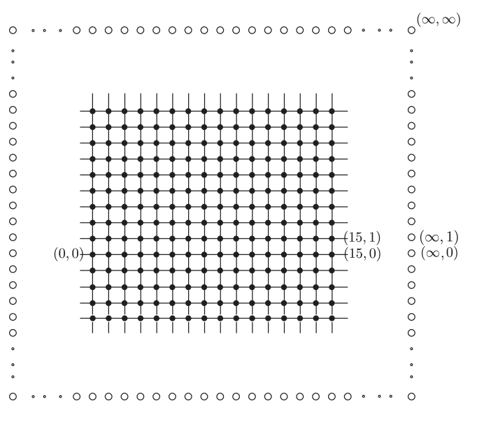
Figure 1. The Euclidean plane with admissable vertices attached

2.1 Lemma.

An element $z$ of the Hamming cube is an admissible vertex if and only if for every $n\geq 2$ and every collection of $n$ hyperplanes $H_{1},\dots,H_{n}$ there exists an original vertex $x$ satisfying $x(H_{i})=z(H_{i})$, for each $i=1,\dots,n$.

Proof.

We are concerned with the forward implication, which we prove by induction on $n$. The case $n=2$ is covered by the definition of an admissible vertex. Let $n>2$ and let $H_{1},\dots,H_{n}$ be $n$ hyperplanes. By the induction hypothesis we have an original vertex $x_{1}$ agreeing with $z$ on $H_{1},\dots,H_{n-1}$, another original vertex $x_{2}$ agreeing with $z$ on $H_{2},\dots,H_{n}$, and a third original vertex $x_{3}$ agreeing with $z$ on $H_{1}$ and $H_{n}$. The median $m(x_{1},x_{2},x_{3})$ has the desired property. ∎

2.2 Proposition.

The closure $\overline{X}$ of the set of original vertices is the set of admissible vertices.

Proof.

Lemma 2.1 shows that every basic open neighborhood of an admissible vertex contains an original vertex. Thus, every admissible vertex is in the closure of the original vertices.

Conversely, suppose $z$ belongs to the closure of the original vertices, and let $H$ and $K$ be hyperplanes. The requirements $x(H)=z(H)$ and $x(K)=z(K)$ define an open neighborhood of $z$ in the infinite product, so must contain an original vertex. Hence $z$ is admissable. ∎

We extend the above terminology regarding hyperplanes and half spaces to $\overline{X}$ in the obvious way. For example, an admissible vertex $z$ belongs to the half space $H^{+}$ if $z(H)=+1$; it belongs to $H^{-}$ if $z(H)=-1$. Thus, we extend the half spaces to include ideal vertices. Having extended the notion of half space to the set of admissable vertices we define intervals exactly as before, as intersections of half spaces. In later sections we shall work onlywith intervals $[x,z]$ in which $x$ is an original vertex, whereas $z$ may be either an original or an ideal vertex.

A pair of admissible vertices $z$ and $w$ are separated by the hyperplane $H$ when $z(H)\neq w(H)$. While only finitely many hyperplanes may separate a pair of original vertices, a pair of vertices at least one of which is ideal may be separated by infinitely many hyperplanes. For example, in Figure 1 the ideal vertices $(\infty,0)$ and $(\infty,1)$ are separated by a single hyperplane, whereas the ideal vertices $(\infty,0)$ and $(\infty,\infty)$ are separated by infinitely many horizontal hyperplanes.

A pair of admissable vertices $z$ and $w$ are adjacent across the hyperplane $H$ if they differ only on $H$. An admissable vertex $z$ is adjacent to the hyperplane $H$ if there is an admissable vertex $w$ such that $z$ is adjacent to $w$ across $H$.

2.3 Proposition.

Let $x$, $y$ and $z$ be admissible vertices. The element of the Hamming cube defined by

$$m(H)=\begin{cases}+1,&\text{at least two of\/ $x(H)$, $y(H)$, $z(H)=1$}\\ -1,&\text{at least two of\/ $x(H)$, $y(H)$, $z(H)=-1$}\end{cases}$$

is an admissible vertex. It is the unique admissible vertex belonging to all three of the intervals $[x,y]$, $[y,z]$ and $[x,z]$.

Proof.

We first check that $m$ is admissible. Suppose hyperplanes $H$ and $K$ are given. At least two of the vertices $x$, $y$, $z$ must agree with $m$ on $H$ and at least two must agree with $m$ on $K$, so at least one agrees with $m$ on both $H$ and $K$. Since that vertex is itself admissable there is an original vertex which agrees with $m$ on both $H$ and $K$.

We next check that $m$ belongs to the interval $[x,y]$. Indeed, if $H$ separates $m$ from both $x$ and $y$ then $x(H)=y(H)\neq m(H)$, contradicting the definition of $m$. The other intervals are treated similarly.

Finally, we verify uniqueness. Suppose $m^{\prime}$ is an admissible vertex belonging to each of the intervals $[x,y]$, $[y,z]$ and $[x,z]$. Given a hyperplane $H$ at least two of the vertices $x$, $y$ and $z$ belong to a common half space of $H$. Thus, $m^{\prime}$ agrees with at least two of the vertices $x$, $y$ and $z$ on $H$ so that $m^{\prime}$ agrees with $m$ on $H$ as well. As the hyperplane $H$ was arbitrary, we conclude that $m^{\prime}=m$. ∎

The proposition extends the notion of median to admissible vertices: the admissible vertex $m$ described in the statement is the median of the three admissable vertices $x$, $y$ and $z$; as with medians of original vertices we write $m=m(x,y,z)$.

We close this section with some elementary remarks concerning the topological space $\overline{X}$. Each half space is a clopen set. The collection of finite intersections of half spaces comprises a basis for the topology on $\overline{X}$. For an admissible vertex $z$, the singleton $\{\,z\,\}$ is closed; if $z$ is an ideal vertex $\{\,z\,\}$ is not open. For original vertices the situation is more complicated.

2.4 Proposition.

Let $x$ be an original vertex. The following are equivalent:

• $\{\,x\,\}$ is open in $\overline{X}$;

• $\{\,x\,\}$ is open in $X$ with respect to the subspace topology;

• $x$ is a finite vertex.

Here, an original vertex is said to be finite if there are only finitely many hyperplanes adjacent to it. It follows that, in the case of a non-locally finite complex, $X$ itself has non-trivial topology as a subspace of $\overline{X}$ – that is, the subspace topology on $X$ is not discrete.

Proof.

Elementary topology shows that (1) implies (2), and (2) implies (3). If $x$ is a finite vertex, and $H_{1},\dots,H_{n}$ are the (finitely many) hyperplanes adjacent to $x$ then we claim that

(2.1) $$\{\,x\,\}=H_{1}^{x(H_{1})}\cap\dots\cap H_{n}^{x(H_{n})},$$

which is a basic open set for the topology on $\overline{X}$. To verify (2.1) we must, according to our conventions, show that no admissible vertex other than $x$ can belong to the displayed intersection of half spaces. It is an elementary fact that the intersection can contain no original vertex other than $x$. Thus, we must show that the intersection can contain no ideal vertex. Suppose that $z$ is an ideal vertex which agrees with $x$ on the given hyperplanes. Necessarily, $z$ differs from $x$ on some other hyperplane $K$. By Lemma 2.1 there is an original vertex $y$ which agrees with $z$ on the hyperplanes $H_{1},\dots,H_{n}$, and also on $K$. Thus, $y$ is an original vertex that agrees with $x$ on $H_{1},\dots,H_{n}$ but differs from it on $K$, a contradiction. ∎

While $\overline{X}$ is a compact space containing $X$ as a dense subspace, it is not in general a compactification of $X$ in the classical sense – when $X$ is not locally finite it need not be an open subset of $\overline{X}$. We shall not require this fact below, and its verification is left to the reader. (But, compare to the discussion surrounding Propositions 3.4 and 3.6.)

2.5 Proposition.

The compact space $\overline{X}$ contains $X$ as a dense subspace. An action of a discrete group on $X$ by cellular automorphisms extends to an action on $\overline{X}$ by homeomorphisms.

Proof.

Open sets in $\overline{X}$ are unions of finite intersections of half spaces all of which contain original vertices by Lemma 2.1, so $X$ is dense in $\overline{X}$ as required. An automorphism of $X$ preserves the half space structure and therefore extends to a homeomorphism of $\overline{X}$. ∎

3. Weight functions

Let $X$ be the vertex set of a finite dimensional $\operatorname{CAT}(0)$ cube complex. In previous work we constructed weight functions on $X$ – we used these to show that $X$ has Property $A$, when viewed as a metric space with either of its natural metrics [3]. We shall use the previously constructed weight functions in the present context as well, and now recall their definition.

Fix an ambient dimension $N$ greater than or equal to the dimension of the complex. For every $z\in\overline{X}$ and every vertex $a\in[x,z]\cap X$ the deficiency of $a$ (relative to the interval $[x,z]$) is

(3.1) $$\delta_{[x,z]}(a)=N-k,$$

where $k$ is the number of hyperplanes cutting edges adjacent to $a$ and which separate $a$ (and hence also $x$) from $z$. By hypothesis $0\leq\delta_{[x,z]}(a)\leq N$. Now for every vertex $x\in X$ and every $z\in\overline{X}$ we define the weight function $\phi^{n}_{x,z}$ according to the formula

(3.2) $$\phi^{n}_{x,z}(a)=\begin{cases}{n-d(x,a)+\delta_{[x,z]}(a)\choose\delta_{[x,z]}(a)},&a\in[x,z]\\ 0,&a\notin[x,z].\end{cases}$$

Intuitively $\phi^{n}_{x,z}$ measures the flow of a mass placed at the vertex $x$ as it flows towards $z$ with $n$ playing the role of the time parameter. The basic properties of the weight functions are summarized in the following theorem [3]. In the statement, $B_{n}(x)$ denotes the ball of radius $n$ and center $x$, comprised of those (original) vertices separated from $x$ by at most $n$ hyperplanes; the norms are $\ell_{1}$-norms.

3.1 Theorem.

Let $X$ be the vertex set of a finite dimensional $\operatorname{CAT}(0)$ cube complex, and let $\overline{X}$ be the compact space of admissible vertices, defined previously. Fix an ambient dimension $N$ not less than the dimension of $X$. The weight functions

$$\phi^{n}:X\times\overline{X}\to\ell_{1}(X),\quad(x,z)\mapsto\phi^{n}_{x,z}$$

defined by formula (3.2) satisfy the following:

• $\phi^{n}_{x,z}$ is $\mathbb{N}\cup\{0\}$-valued;

• $\phi^{n}_{x,z}$ is supported in $B_{n}(x)\cap[x,z]$;

• $\|\phi^{n}_{x,z}\|={n+N\choose N}$;

• if $x$ and $x^{\prime}\in X$ are adjacent then $\|\phi^{n}_{x,z}-\phi^{n}_{x^{\prime}z}\|=2{n+N-1\choose N-1}$.

Further, if a discrete group $\Gamma$ acts cellularly on $X$, hence also by homeomorphisms on $\overline{X}$, we have

• $s\cdot\phi^{n}_{x,z}=\phi^{n}_{sx,sz}$ ,

for every $s\in\Gamma$.

Proof.

Properties, (1) and (2) are immediate from the defining formula (3.2). Property (5) is also apparent from the defining formula – indeed, it is equivalent to the assertion that

$$\phi^{n}_{x,z}(a)=\phi^{n}_{sx,sz}(sa),$$

for all $x$, $a\in X$, $z\in\overline{X}$ and $s\in\Gamma$, which holds since $\Gamma$ acts cellularly and the weight functions are determined by the combinatorics of hyperplanes. Finally, properties (3) and (4) are established in Propositions 2.3 and 2.4 of [3]. ∎

The remainder of the section is devoted to an analysis of the continuity properties of the weight functions defined in (3.2). In particular, we shall view $\phi^{n}_{x,z}(a)$, as a function of $z\in\overline{X}$, for a fixed natural number $n$, and for fixed $x$ and $a\in X$. Our first result in this direction is the following proposition.

3.2 Proposition.

Fix a natural number $n$, and original vertices $x$ and $a\in X$. The function

$$\Phi:\overline{X}\to\mathbb{N},\qquad\Phi(z)=\phi^{n}_{x,z}(a).$$

satisfies the following:

• if $n\leq d(x,a)$ then $\Phi$ is continuous;

• if $n>d(x,a)$ and

  • $a$ is finite then $\Phi$ is continuous;

  • $a$ is not finite then $\Phi$ is Borel.

Before turning to the proof of the proposition, we require a lemma.

3.3 Lemma.

For any choice of original vertices $x$ and $a$ the set $\{\,z:a\in[x,z]\,\}$ is clopen in $\overline{X}$.

Proof.

The complement of the set in question is

$$\{\,z:\text{$\exists$ $H\in\mathcal{H}$ such that $H$ separates $a$ from both $x$ and $z$}\,\}=\cup H^{x(H)},$$

where the union is over the finite set of hyperplanes separating $a$ from $x$. (When $a=x$ this set is empty.) This set is clopen, hence so is its complement. ∎

Proof of Proposition 3.2.

We divide (1) into two cases. First, if $n<d(x,a)$ then $\Phi$ is identically zero. Second, if $n=d(x,a)$ then $\Phi$ is given by the formula

$$\Phi(z)=\begin{cases}1,&a\in[x,z]\\ 0,&\text{else}.\end{cases}$$

In other words, $\Phi$ is the characteristic function of the clopen set appearing in the previous lemma, and so it is continuous.

We consider (2a) and (2b) simultaneously, and proceed by analysing the level sets of $\Phi$.

Write $A=n-d(x,a)>0$. Inspecting (3.2) we see that $\Phi$ is given by the formula

$$\Phi(z)=\begin{cases}{A+(N-k)\choose(N-k)},&a\in[x,z]\\ 0,&a\notin[x,z],\end{cases}$$

where $k=k(z)$ appears in the formula (3.1) for the deficiency. Thus, the values of $\Phi$ are among the (distinct) natural numbers

$$0\quad\text{and}\quad{A+(N-k)\choose(N-k)},\quad 0\leq k\leq\dim(X)\leq N.$$

Further, the level sets corresponding to these values are $\Phi^{-1}(0)=\{\,z:a\notin[x,z]\,\}$ and

(3.3) $$\Phi^{-1}\left({A+(N-k)\choose(N-k)}\right)=\{\,z:\text{$a\in[x,z]$ and $\delta_{[x,z]}(a)=N-k$}\,\},$$

respectively. The first of these is clopen, by the lemma. We analyze the second (3.3).

Let $K_{1},\dots,K_{n}$ be the (finitely many) hyperplanes separating $x$ and $a$. Let $H_{1},H_{2},\dots$ be the hyperplanes adjacent to $a$ and not separating $x$ and $a$. Observe the the collection of $H$’s is finite exactly when $a$ is a finite vertex. The conditions defining the level set (3.3) are that $x$ and $z$ are separated by every $K_{i}$ and exactly $k$ of the $H_{j}$. Similarly,

(3.4) $$\Phi(z)>{A+(N-k)\choose(N-k)}$$

precisely when $x$ and $z$ are separated by every $K_{i}$ and fewer than $k$ of the $H_{j}$. Thus, the set of admissible $z$ satisfying (3.4) is precisely

(3.5) $$K_{1}^{a(K_{1})}\cap\dots\cap K_{n}^{a(K_{n})}\cap\bigcap\left(H_{j_{1}}^{x(H_{j_{1}})}\cup\dots\cup H_{j_{k}}^{x(H_{j_{k}})}\right),$$

with the large intersection being over the $k$ element subsets $j_{1},\dots,j_{k}$ of $j$’s. The set appearing in (3.5) is closed so that, as the difference of two closed sets, the level set (3.3) is Borel, as is $\Phi$. Further, if $a$ is finite, the set appearing in (3.5) is clopen – the intersection is finite because there are only finitely many $k$ element subsets of $j$’s. In this case, as the difference of clopen sets, the level set (3.3) is clopen and $\Phi$ is continuous. ∎

Remark.

In the course of the proof we have established the following fact: for all choices of the parameters $n$, $x$ and $a$, if $\Phi(z)=0$ then $\Phi$ is continuous at $z$.

Remark.

The proposition leaves open the question of whether $\Phi$ is continuous when $a$ is an infinite point. Indeed, it is not difficult to see that if $a$ is infinite then $\Phi$ is not continuous.

In the notation of the proposition, suppose that $a$ is an infinite point (and also that $n>d(x,a)$). We show that $\Phi$ is not continuous at $a$. Indeed, let $H_{1},H_{2},\dots$ be an infinite sequence of hyperplanes adjacent to $a$, none of which separate $a$ from $x$. Let $z_{j}$ be the vertex immediately across $H_{j}$ from $a$, and note that $a\in[x,z_{j}]$. Inspecting the definition (3.2) we see that

$$\Phi(a)={n-d(x,a)+(N-0)\choose(N-0)}\neq{n-d(x,a)+(N-1)\choose N-1}=\Phi(z_{j}).$$

The value $\Phi(z_{j})$ is independent of $j$, different from $\Phi(a)$ and $z_{j}\to a$.

While this remark is quite simple, it leads to a complete analysis of the continuity of the $\Phi$, which we develop in the two subsequent propositions. Note that when $z=a$ the first of these is essentially the previous remark.

3.4 Proposition.

Continue in the notation of Proposition 3.2, and assume $n>d(x,a)$. Let $z$ be an original vertex for which $\Phi(z)\neq 0$. The function $\Phi$ is continuous at $z$ exactly when only finitely many hyperplanes are adjacent to both $a$ and $z$.

Proof.

The forward implication proceeds exactly as the remark. Indeed, with $z$ as in the statement, let $H_{1},H_{2},\dots$ be an infinite sequence of hyperplanes adjacent to both $a$ and $z$, none of which separate $a$ from $z$, and none of which separate $a$ from $x$. The vertices $z_{j}$ immediately across $H_{j}$ from $z$ witness the non-continuity of $\Phi$ at $z$.

For the reverse implication, let $H_{1},\dots,H_{n}$ be the hyperplanes adjacent to both $a$ and $z$, and let $K_{1},\dots,K_{m}$ be the hyperplanes that separate $x$ and $z$. The intersection

$$H_{1}^{z(H_{1})}\cap\dots\cap H_{n}^{z(H_{n})}\cap K_{1}^{z(K_{1})}\cap\dots\cap K_{m}^{z(K_{m})}$$

is a clopen neighborhood of $z$. Let $w$ belong to this neighborhood. We claim that $\Phi(w)=\Phi(z)$. Now, since $w\in K_{i}^{z(K_{i})}$ for all $i$ we have $a\in[x,w]$. Thus, the values $\Phi(w)$ and $\Phi(z)$ are given by the first case in (3.2) and we must show

$$\delta_{[x,z]}(a)=\delta_{[x,w]}(a).$$

We introduce the notation $\mathfrak{N}_{z}(a)$ for the deficiency set of $a$ with respect to $z$, that is, the set of hyperplanes that are adjacent to $a$ and that separate $a$ from $z$. The deficiency $\delta_{[x,z]}(a)$ is the difference of $N$ and the cardinality of $\mathfrak{N}_{z}(a)$. Thus, it suffices to show that $\mathfrak{N}_{z}(a)=\mathfrak{N}_{w}(a)$.

Because $a\in[x,z]$ (by hypothesis), a hyperplane separating $a$ and $z$ is one of the $K_{i}$, which therefore also separates $a$ from $w$. It follows that $\mathfrak{N}_{z}(a)\subset\mathfrak{N}_{w}(a)$. For the reverse inclusion, suppose $H\in\mathfrak{N}_{w}(a)$. We must show that $H$ separates $a$ from $z$. If not, then the subsequent lemma shows that $H$ is adjacent to $z$ – indeed, $z\in[a,w]$ since any hyperplane separating $a$ from $z$ also separates $x$ from $z$, thus is among the $K_{i}$. Thus, $H$ is one of the $H_{j}$, so that $z$ and $w$ are on the same side of $H$, the side opposite $a$. This is a contradiction. ∎

3.5 Lemma.

Suppose that $H$ is adjacent to $a$, that $H$ separates $z$ and $w$, and that $z\in[a,w]$. Then $z$ is adjacent to $H$.

Proof.

Observe that $H$ separates $a$ from $w$, and hence not from $z$; indeed, otherwise $H$ separates both $a$ and $w$ from $z$ contradicing $z\in[a,w]$. Let $b$ be the vertex immediately across $H$ from $a$. Let $m$ be the median of $b$, $z$ and $w$. We claim that $H$ is the unique hyperplane separating $z$ from $m$ so that, in particular, $z$ is adjacent to $H$. Indeed,

$$w(H)=b(H)\neq a(H)=z(H)$$

shows that $m(H)\neq z(H)$, that is, $H$ separates $m$ and $z$. Further, if $K$ is such that $z(K)\neq m(K)$ then

$$b(K)=w(K)=m(K)\neq z(K)=a(K),$$

where the last equality holds since $a\in[a,w]$. Thus, $K$ separates $a$ from $b$, and $K=H$. ∎

Continuity of $\Phi$ at ideal vertices is slightly more subtle, and is treated in the next proposition. Observe that when $z$ is an original vertex, the stated condition reduces to the one in the previous proposition – indeed, when $z$ is an original vertex elements of the interval $[a,z]$ can only be separated from $z$ by those (finitely many) hyperplanes that separate $a$ from $z$; thus, any sequence of such points converging to $z$ is eventually constant.

3.6 Proposition.

Continue in the notation of Proposition 3.2, and assume $n>d(x,a)$. Let $z$ be an admissible vertex for which $\Phi(z)\neq 0$. The function $\Phi$ is not continuous at $z$ precisely when there is a sequence $m_{1},m_{2},\dots$ of admissable vertices in the interval $[a,z]$ converging to $z$ and a sequence $H_{1},H_{2},\dots$ of distinct hyperplanes adjacent to $a$ for which $H_{j}$ is adjacent to $m_{j}$.

Proof.

We provide Figure 2 to aid the reader in following the proof.

Suppose first that $\Phi$ is not continuous at $z$, and that $\Phi(z)\neq 0$. We claim that there exists a sequence of admissible vertices $z_{j}\to z$ such that every $z_{j}$ satisfies the following:

• $a\in[x,z_{j}]$

• $\delta_{[x,z_{j}]}(a)\neq\delta_{[x,z]}(a)$.

Indeed, begin with a sequence $z_{j}\to z$ for which $\Phi(z_{j})$ does not converge to $\Phi(z)$. Now, every sequence of admissible vertices converging to $z$ must satisfy (1) on a tail – $\Phi(z)\neq 0$ implies that $z$ belongs to the clopen set described in Lemma 3.3. Thus, we may assume our sequence satisfies (1), so that the values $\Phi(z_{j})$ are given by the first case in (3.2). Thus, $\delta_{[x,z_{j}]}(a)$ does not converge to $\delta_{[x,z]}(a)$ and, we arrange for (2) by passing to a subsequence.

Consider now the median

(3.6) $$m_{j}=m(a,z_{j},z),$$

which by construction lies in the interval $[a,z]$. As shown in [3] the sequence $m_{j}$ converges to $z$. The $m_{j}$ (rather, a subsequence) will be the sequence we seek – it remains to locate the required adjacent hyperplanes. To do this, we claim that for sufficiently large $j$, we have $\mathfrak{N}_{m_{j}}(a)\neq\mathfrak{N}_{z_{j}}(a)$ – here, we employ the notation regarding deficiency sets introduced in the proof of Proposition 3.4. Again as shown in [3], since the $m_{j}$ converge to $z$ and lie in the interval $[a,z]$, the subsets $\mathfrak{N}_{m_{j}}(a)$ eventually stabilise at $\mathfrak{N}_{z}(a)$. Thus, combined with (2) we see that for sufficiently large $j$

$$\delta_{[x,m_{j}]}(a)=\delta_{[x,z]}(a)\neq\delta_{[x,z_{j}]}(a),$$

from which the claim follows. Thus, for each sufficiently large $j$ there is a hyperplane $H_{j}$ adjacent to $a$ that separates $m_{j}$ and $z_{j}$. It follows from Lemma 3.5 that $H_{j}$ is adjacent to $m_{j}$ – by (3.6) we have $m_{j}\in[a,z_{j}]$ so that the lemma applies.

It remains only to see that the sequence $H_{j}$ contains infinitely many distinct hyperplanes. Indeed, we shall show slightly more – that every hyperplane $H$ can appear as an $H_{j}$ only finitely many times. Assume to the contrary, that the hyperplane $H$ appears infinitely many times. Then, since both $z_{j}$ and $m_{j}$ converge to $z$, they are eventually on a common side of $H$, which contradicts the fact that $H$ separates $m_{j}$ and $z_{j}$.

Suppose now that $\Phi(z)\neq 0$ and that the conditions in the statement are satisfied. We are to show that $\Phi$ is not continuous at $z$. As remarked above, since the $m_{j}$ converge to $z$ and all belong to the interval $[a,z]$, the deficiency sets $\mathfrak{N}_{m_{j}}(a)$ eventually stabilise at $\mathfrak{N}_{z}(a)$ [3]; without loss of generality we may assume that they all coincide. Let $m_{j}^{\prime}$ denote the vertex immediately across $H_{j}$ from $m_{j}$. We claim that $m^{\prime}_{j}$ converges to $z$. To see this, let $K$ be an arbitrary hyperplane. If $K$ is not one of the $H_{j}$ then $m^{\prime}_{j}$ and $m_{j}$ agree on $K$ for every $j$; if $K$ is one of the $H_{j}$ then $m^{\prime}_{j}$ and $m_{j}$ agree on $K$ for sufficiently large $j$. Either way, $m^{\prime}_{j}$ and $z$ will agree on $K$ for sufficiently large $j$ as this is the case for $m_{j}$.

It remains to show that $\Phi(m^{\prime}_{j})$ does not converge to $\Phi(z)$. Comparing to the beginning of the proof, the value $\Phi(m^{\prime}_{j})$ is given by the first case in (3.2). Thus, we must show that deficiencies $\delta_{[x,m^{\prime}_{j}]}(a)$ do not converge to $\delta_{[x,z]}(a)$. To see this we note that for each $j$, the deficiency sets $\mathfrak{N}_{m_{j}}(a)$ and $\mathfrak{N}_{m_{j}^{\prime}}(a)$ differ in at exactly one place, either including or deleting $H_{j}$ from the set. It follows that $\delta_{[x,{m_{j}^{\prime}}]}(a)=\delta_{[x,m_{j}]}(a)\pm 1=\delta_{[x,z]}(a)\pm 1\not=\delta_{[x,z]}(a)$ and the proof is complete. ∎

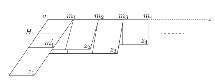
Figure 2. A point $z$ at which the weight function $\Phi$ is not continuous.

Remark.

Let $X$ be a (simplicial) tree. Taken together, the previous propositions show that for fixed vertices $x$ and $a\in X$, the function $\Phi(z)$ is continuous on all of $\overline{X}$, except possibly at $a$ itself. Further, it is continuous at $a$ exactly when $a$ is finite.

In summary, when the cube complex is locally finite (that is, every original vertex is finite) the weight functions are continuous; in general, however, they are merely Borel. In either case we shall need to renormalise to produce probability measures indexed by $\overline{X}$ while in the latter case we shall also need to replace the Borel weight functions by a continuous family of probability measures. Renormalisation is easy since the weight functions are all non-negative and have $\ell^{1}$ norm equal to ${n+N\choose N}$ by Theorem 3.1. Further, the normalised weight functions ${n+N\choose N}^{-1}\phi^{n}_{x,z}$ share the same continuity and Borel properties as the original $\phi^{n}_{x,z}$. Obtaining a continuous family of weight functions is more difficult, but understood. The following result is based on the methods of [4, 14].

3.7 Lemma.

Let $G$ be a group acting by cellular isometries on a finite dimensional $\operatorname{CAT}(0)$ cube complex $X$. Given a finite subset $E\subset\Gamma$ and $\varepsilon>0$, there is a finite subset $F\subset X$ and a function $\eta:\overline{X}\rightarrow{\operatorname{Prob}(X)}$ such that

• $\eta_{z}(a)$ is continuous in $z$, for each $a\in{X}$;

• $\operatorname{supp}\eta_{z}\subset F$, for every $z\in{\overline{X}}$;

• $\|s\cdot\eta_{z}-\eta_{sz}\|<\varepsilon$, for every $s\in E$ and every $z\in\overline{X}$.

Sketch of proof.

We sketch the argument of Ozawa, refering to [4, Section 5.2] for details.

When $X$ is locally finite there is nothing to prove. Fixing a basepoint $x\in X$ define $\eta$ using the normalized weight functions: $\eta_{z}(a)={n+N\choose N}^{-1}\phi^{n}_{z,x}(a)$.

When $X$ is not locally finite the normalised weight functions are neither continuous in $z$, nor do they satisfy the conclusion (2) on unifom supports. They are, however, Borel and the proof proceeds by applying Lusin’s theorem to approximate them by appropriate continuous functions $\eta_{z}$, taking care to ensure that we truncate to a common finite subset $F$ throughout. The approximation is carried out so that $0\in C(\overline{X})$ is in the weak closure of the $s\cdot\eta_{z}-\eta_{sz}$. Applying the Hahn-Banach theorem, after taking convex combinations we obtain (3).

∎

Remark.

In fact, we shall not require the full statement of the lemma. We require only the existence, for every finite subset $E$ and $\varepsilon>0$, of a finite subset $F$ and functions $\eta:X\to\operatorname{Prob}(X)$ satisfying (2) and (3) where in (3) we consider only those $z\in X$.

4. Permanence

We shall adopt the following characterization of Property $A$ as our definition. A countable discrete group $\Gamma$ has Property $A$ if for every finite subset $E\subset\Gamma$ and every $\varepsilon>0$ there exists a finite subset $F\subset\Gamma$ and a function $\nu:\Gamma\to\operatorname{Prob}(\Gamma)$ such that

• $\operatorname{supp}\nu_{x}\subset F$, for every $x\in\Gamma$,

• $\|s\cdot\nu_{x}-\nu_{sx}\|<\varepsilon$, for every $s\in E$ and every $x\in\Gamma$.

Here, $\operatorname{Prob}(\Gamma)$ is the space of probability measures on $\Gamma$ and the norm is the $\ell_{1}$-norm. We refer to [11, Lemma 3.5] for the equivalence with the original formulation of Property $A$ found in [16]. For the present purposes our definition has two advantages; first it makes no reference to a particular compact space on which the group acts, and second the probability measure associated to a particular $x\in\Gamma$ is supported near the identity of $\Gamma$ and not near $x$ itself.

4.1 Theorem.

Let $\Gamma$ be a countable discrete group acting on a finite dimensional cubical complex $X$. Then $\Gamma$ has Property $A$ if and only if every vertex stabilizer of the action has Property $A$.

Since every subgroup of a Property $A$ group has Property $A$ we only need to prove that if every vertex stabliser has Property $A$ then so does $\Gamma$. To do so we will have to inflate the Property $A$ functions for the stabilisers to functions defined on the whole group. After first establishing relevant notation, we shall accomplish this in the next lemma.

Let $\Delta$ be a subgroup of a group $\Gamma$. Choose a set $Z$ of coset representatives for the right cosets of $\Delta$ in $\Gamma$. Thus, every $g\in\Gamma$ has a unique representation

$$g=z_{g}a_{g},\quad\text{$z_{g}\in Z$, $a_{g}\in\Delta$}.$$

These satisfy the following properties:

$$z_{gk}(a_{gk}a_{k}^{-1}) = gz_{k},\quad\text{for $g$, $k\in\Gamma$}$$

(4.1) $$a_{gh} = a_{g}h,\quad\text{for $g\in\Gamma$, $h\in\Delta$}$$

$$z_{gh} = z_{g},\quad\text{for $g\in\Gamma$, $h\in\Delta$};$$

indeed, the first follows from $z_{gk}a_{gk}=gk=gz_{k}a_{k}$ and the others from $z_{gh}a_{gh}=gh=z_{g}a_{g}h$ together with $a_{g}h\in\Delta$.

4.2 Lemma.

Suppose $\Delta$ is a subgroup of a group $\Gamma$ and that $\Delta$ has Property $A$. For every finite subset $E\subset\Delta$ and every $\varepsilon>0$ there exists a finite subset $F\subset\Delta$ and a function $\nu:\Gamma\to\operatorname{Prob}(\Gamma)$ such that

• $\operatorname{supp}(\nu_{g})\subset F$, for every $g\in\Gamma$,

• $\|h\cdot\nu_{g}-\nu_{hg}\|<\varepsilon$, for every $h\in E$ and every $g\in\Gamma$.

Proof.

We shall lift functions obtained from the assumption that $\Delta$ has Property $A$ from $\Delta$ to $\Gamma$ using a $\Delta$-equivariant splitting of the inclusion $\Delta\subset\Gamma$; we consider $\Delta$ acting on the left of both $\Delta$ and $\Gamma$. Precisely, define

$$\sigma:\Gamma\to\Delta,\quad\sigma(g)=a_{g^{-1}}^{-1}$$

and observe that if $h\in\Delta$ we have

$$\sigma(hg)=a_{g^{-1}h^{-1}}^{-1}=(a_{g^{-1}}h^{-1})^{-1}=ha_{g^{-1}}^{-1}=h\sigma(g),$$

where the second equality follows from (4.1). If now $E$ and $\varepsilon$ are given, we obtain a function $\Delta\to\operatorname{Prob}(\Delta)$ as in the definition of Property $A$ and define $\nu$ to be the composition

$$\Gamma\to\Delta\to\operatorname{Prob}(\Delta)\subset\operatorname{Prob}(\Gamma),$$

in which the first map is our splitting $\sigma$ and we simply view $\operatorname{Prob}(\Delta)$ as the probability measures on $\Gamma$ which are supported on $\Delta$. The required properties are easily verified, with left $\Delta$-equivariance of $\sigma$ used to verify the norm inequality. ∎

Now suppose that $\Gamma$ acts on a CAT(0) cube complex by cellular isometries. As above we obtain an induced continuous action on the space $\overline{X}$ of admissible vertices. Fix a transversal $T$ for the action of $\Gamma$ on $X$; thus, $T\subset X$ contains exactly one point from each $\Gamma$-orbit. We do not assume that $T$ is finite. Denote the stabiliser of $t\in T$ by $\Gamma^{t}$. We apply the previous notational conventions to $\Gamma^{t}$. In particular, fixing a set of coset representatives $Z^{t}$ for $\Gamma^{t}$ in $\Gamma$ we have decompositions

$$g=z_{g}a_{g}$$

as above, and the previous lemma applies. As these decompositions depend on $t\in T$, we should more properly include $t$ in the notation and write, for example $g=z_{g}^{t}a_{g}^{t}$. Observe

$$g\cdot t=z_{g}a_{g}\cdot t=z_{g}\cdot t.$$

Thus, the orbit map $g\mapsto g\cdot t$ restricts to a map $Z^{t}\to X$, which is a bijection of $Z^{t}$ onto the orbit $\Gamma t$ of $t$.

Proof of Theorem 4.1.

We are given a finite subset $E\subset\Gamma$ and $\varepsilon>0$. Without loss of generality we assume that $E$ is closed under inversion and contains the identity of $\Gamma$. We must produce a finite subset $F\subset\Gamma$ and a function $\nu:\Gamma\to\operatorname{Prob}(\Gamma)$ as in the definition of Property $A$.

Applying Lemma 3.7 (or, more properly, the subsequent remark) there is a finite subset $F\subset X$ and a function $\eta:X\rightarrow\operatorname{Prob}(X)$ such that

• $\operatorname{supp}\eta_{x}\subset F$, for every $x\in X$;

• $\|s\cdot\eta_{x}-\eta_{sx}\|<\varepsilon$, for every $s\in E$ and every $x\in X$.

Let $T_{F}\subset T$ be the (finite) set of representatives of those orbits passing through $F$; in other words, $t\in T_{F}$ precisely when $\Gamma\cdot t\cap F$ is nonempty. For each $t\in T_{F}$ let $Z^{t}_{F}\subset Z^{t}$ be the (finite) subset of representatives of those $\Gamma^{t}$ cosets mapping $t$ into $F$; in other words, $z\in Z^{t}_{F}$ precisely when $z\cdot t\in F$. Recall here that the action on $t$ restricted to coset representatives provides a bijection of $Z^{t}$ with the orbit $\Gamma\cdot t$. Let $E^{t}\subset\Gamma^{t}$ be the (finite) subset

$$E^{t}=\{\,z^{-1}_{sg}sz_{g}:\text{$s\in E$, $g\in Z^{t}_{F}$}\,\}.$$

For each $t\in T_{F}$, using the hypothesis on $\Gamma^{t}$ apply Lemma 4.2 with $\Delta=\Gamma^{t}$ and $E=E^{t}$ to obtain a finite subset $F_{t}\subset\Gamma^{t}$ and a function $\nu^{t}:\Gamma\to\operatorname{Prob}(\Gamma)$ such that

• $\operatorname{supp}\nu^{t}_{g}\subset F_{t}$, for every $g\in\Gamma$;

• $\|h\cdot\nu^{t}_{g}-\nu^{t}_{hg}\|<\varepsilon$, for every $h\in E^{t}$ and $g\in\Gamma$.

Define the required function $\mu:\Gamma\to\operatorname{Prob}(\Gamma)$ by choosing a vertex $O$ as a basepoint and setting, for each $x$ and $g\in\Gamma$,

(4.2) $$\mu_{x}(g)=\sum_{t\in T}\eta_{x\cdot O}(g\cdot t)\,\nu^{t}_{z^{-1}_{g}x}(a_{g}).$$

Observe that the sum is actually finite as only finitely many orbits can cross the (finite) common support $F$ of the $\eta_{x\cdot O}$; indeed, the sum is over $t\in T_{F}$.

Let us first address the finiteness of support. For $\mu_{x}(g)$ to be nonzero, there must be $t\in T_{F}$ for which both factors of the corresponding summand in (4.2) are nonzero. Fixing such a $t$ and decomposing $g=z_{g}a_{g}$ accordingly we obtain: $z_{g}\cdot t=g\cdot t\in F$ so that $z_{g}\in Z^{t}_{F}$, and also $a_{g}\in F_{t}$. It follows that

$$\operatorname{supp}\mu_{x}\subset\bigcup_{t\in T_{F}}Z^{t}_{F}F_{t},$$

which is a finite subset of $\Gamma$, not depending on $x$.

Let us next check that each $\mu_{x}$ is a probability measure. For these and other norm estimates below, we shall reindex sums using the bijection $\Gamma\cong Z^{t}\Gamma^{t}$, possible for each fixed $t\in T$. In other words, having fixed $t\in T$, we shall replace a sum over $g\in\Gamma$ by a double sum over $z\in Z^{t}$ and $g\in z\Gamma^{t}$ and may identify the latter as a sum over $\Gamma^{t}$. We proceed, recalling that $\eta_{x\cdot O}$ and the $\nu^{t}_{(\cdot)}$ are probability measures, hence $[0,1]$-valued,

$$\|\mu_{x}\|_{\ell^{1}(\Gamma)} =\sum_{g\in\Gamma}\mu_{x}(g)=\sum_{g\in\Gamma}\sum_{t\in T}\eta_{x\cdot O}(g\cdot t)\,\nu^{t}_{z^{-1}_{g}x}(a_{g})$$

$$=\sum_{t\in T}\sum_{z\in Z^{t}}\eta_{x\cdot O}(z\cdot t)\sum_{g\in z\Gamma^{t}}\nu^{t}_{z^{-1}x}(a_{g})$$

$$=\sum_{t\in T}\sum_{z\in Z^{t}}\eta_{x\cdot O}(z\cdot t)=\sum_{t\in T}\sum_{y\in\Gamma\cdot t}\eta_{x\cdot O}(y)=1;$$

in the second line we use that $g\cdot t=z\cdot t$ for $g\in z\Gamma^{t}$ and that for $g\in\Gamma$ the condition $g\in z\Gamma^{t}$ is equivalent to $z_{g}=z$; in the third line, observing that the condition $g\in z\Gamma^{t}$ is equivalent to $g=zh$ with $h=a_{g}$ ranging over the stabiliser $\Gamma^{t}$, the sum becomes $\sum_{h\in\Gamma^{t}}\nu^{t}_{z^{-1}x}(h)=1$ since $\nu^{t}_{z^{-1}x}$ is a probability measure; also as $z$ ranges over the coset representatives $Z^{t}$ the value of $z\cdot t$ ranges over the orbit $\Gamma\cdot t$.

Finally, we check the almost invariance condition. We are to estimate

$$\|s\cdot\mu_{x}-\mu_{sx}\|_{\ell^{1}(\Gamma)} =\sum_{g\in\Gamma}|\mu_{x}(s^{-1}g)-\mu_{sx}(g)|$$

$$\leq\sum_{g\in\Gamma}\sum_{t\in T}\bigl{|}\eta_{x\cdot O}(z_{s^{-1}g}\cdot t)\ \nu^{t}_{z^{-1}_{s^{-1}g}x}(a_{s^{-1}g})-\eta_{sx\cdot O}(z_{g}\cdot t)\ \nu^{t}_{z^{-1}_{g}sx}(a_{g})\bigr{|},$$

independent of $x\in\Gamma$ and $s\in E$. We estimate the summand using the triangle inequality

(4.3) $$\eta_{x\cdot O}(z_{s^{-1}g}\cdot t)\left|\nu^{t}_{z^{-1}_{s^{-1}g}x}(a_{s^{-1}g})-\nu^{t}_{z^{-1}_{g}sx}(a_{g})\right|+\left|\eta_{x\cdot O}(z_{s^{-1}g}\cdot t)-\eta_{sx\cdot O}(z_{g}\cdot t)\right|\nu^{t}_{z^{-1}_{g}sx}(a_{g})$$

and shall proceed to estimate each term in this expression (or, more accurately, their sums over $g\in\Gamma$ and $t\in T$). To estimate the term on the right, observe that for $g$ and $h\in\Gamma$ we have that $z_{gh}\cdot t=gh\cdot t=gz_{h}\cdot t$ (where all decompositions are with respect to $\Gamma^{t}$). Hence, fixing $t\in T$ and arguing as above we have

$$\sum_{g\in\Gamma}\left|\eta_{x\cdot O}(z_{s^{-1}g}\cdot t)-\eta_{sx\cdot O}(z_{g}\cdot t)\right|\nu^{t}_{z^{-1}_{g}sx}(a_{g}) =\sum_{g\in\Gamma}\left|\eta_{x\cdot O}(s^{-1}z_{g}\cdot t)-\eta_{sx\cdot O}(z_{g}\cdot t)\right|\nu^{t}_{z^{-1}_{g}sx}(a_{g})$$

$$=\sum_{z\in Z^{t}}\left|\eta_{x\cdot O}(s^{-1}z\cdot t)-\eta_{sx\cdot O}(z\cdot t)\right|\sum_{g\in z\Gamma^{t}}\nu^{t}_{z^{-1}sx}(a_{g})$$

$$=\sum_{z\in Z^{t}}\left|s\cdot\eta_{x\cdot O}(z\cdot t)-\eta_{sx\cdot O}(z\cdot t)\right|.$$

Taking now the sum over $t\in T$ and using the assumption that $s\in E$ we have estimated the right hand term in (4.3) by

$$\|s\cdot\eta_{x\cdot O}-\eta_{sx\cdot O}\|_{\ell^{1}(X)}<\varepsilon.$$

It remains only to estimate the left hand term in (4.3). Again, fix $t\in T$ and reindex the sum over $g\in\Gamma$:

(4.4) $$\sum_{g\in\Gamma}\eta_{x\cdot O}(z_{s^{-1}g}\cdot t) \left|\nu^{t}_{z^{-1}_{s^{-1}g}x}(a_{s^{-1}g})-\nu^{t}_{z^{-1}_{g}sx}(a_{g})\right|=$$

$$=\sum_{z\in Z^{t}}\sum_{g\in z\Gamma^{t}}\eta_{x\cdot O}({s^{-1}z}\cdot t)\left|\nu^{t}_{z^{-1}_{s^{-1}z}x}(a_{s^{-1}g})-\nu^{t}_{z^{-1}sx}(a_{g})\right|;$$

here, we use the fact that for $g\in z\Gamma^{t}$ we have $g\cdot t=z\cdot t$, so that also $z_{s^{-1}g}\cdot t=s^{-1}g\cdot t=s^{-1}z\cdot t$. It follows, in particular, that for $g\in z\Gamma^{t}$ we have $z_{s^{-1}g}=z_{s^{-1}z}$. Hence, setting

$$a=z^{-1}_{s^{-1}g}x=z^{-1}_{s^{-1}z}x,\quad b=z^{-1}_{g}sx=z^{-1}sx,\quad c=ba^{-1}=z^{-1}sz_{s^{-1}z},$$

we see that $a$ and $b$ depend only on $s$, $z$ and $x$, whereas $c$ depends only on $s$ and $z$. The calculation

$$c\cdot t=z^{-1}sz_{s^{-1}g}\cdot t=z^{-1}s{s^{-1}g}\cdot t=z^{-1}g\cdot t=t.$$

shows that $c\in\Gamma^{t}$. Further, we claim that if the summand in (4.4) corresponding to a particular $g\in z\Gamma^{t}$ is nonzero then $c\in E^{t}$. Indeed, if the summand is nonzero then necessarily $s^{-1}z\cdot t\in F$ or, in other words, $h=z_{s^{-1}z}\in Z^{t}_{F}$. Now, by evaluating on $t$ we see that $z_{sh}=z$:

$$z_{sh}\cdot t=sh\cdot t=sz_{s^{-1}z}\cdot t=ss^{-1}z\cdot t=z\cdot t.$$

Hence,

$$c=z^{-1}sz_{s^{-1}z}=z_{sh}^{-1}sh\in E^{t}.$$

Putting everything together, using the final small calculation $a_{g}=ca_{s^{-1}g}$, and summing over the nonzero terms in (4.4) we obtain

$$\sum_{z\in Z^{t}}\eta_{x\cdot O}({s^{-1}z}\cdot t)\sum_{g\in z\Gamma^{t}}\left|\nu^{t}_{a}(c^{-1}a_{g})-\nu^{t}_{ca}(a_{g})\right| =\sum_{z\in Z^{t}}\eta_{x\cdot O}({s^{-1}z}\cdot t)\|c\cdot\nu^{t}_{a}-\nu^{t}_{ca}\|_{\ell^{1}(\Gamma^{t})}$$

$$\leq\varepsilon\sum_{z\in Z^{t}}\eta_{x\cdot O}({s^{-1}z}\cdot t)$$

where the estimate comes from the assumptions on $\nu^{t}$. Summing further over $t\in T$, and recalling that $\eta_{x\cdot O}$ is a probability measure, we have estimated the left hand term in (4.3). ∎

Remark.

The formula used to define $\mu$ in the proof reduces to the formula used in the previous paper [3] in the case when the stabilizers $\Gamma^{t}$ are finite, and the functions $\nu^{t}$ are taken to be constant at the uniform probability measure on $\Gamma^{t}$; in other words,

$$\nu^{t}_{g}(h)=\begin{cases}|\Gamma^{t}|^{-1},&h\in\Gamma^{t}\\ 0,&h\notin\Gamma^{t}.\end{cases}$$

Such $\nu^{t}$ satisfies the conclusions of the previous lemma, so is allowed.

Remark.

Ozawa’s original treatment constructs a space on which $\Gamma$ will act amenably [14]. We have chosen to avoid the formulation in terms of amenable actions because the method seldom produces a reasonable space. It is worth noting, however, that if all stabilisers are finite, or even amenable, $\Gamma$ will act amenably on $\overline{X}$. If, in addition the complex $X$ is locally finite, $\Gamma$ will act amenably on the boundary comprised of ideal vertices.

Remark.

In the locally finite case the result follows from standard permanence results, found for example in [12].

5. Artin groups

A Coxeter matrix is a symmetric matrix $M$, with rows and columns indexed by a not necessarily finite set $I$, and with matrix elements $M_{ij}\in\mathbb{N}\cup\{\infty\}$ satisfying $M_{ii}=1$ for all $i\in I$. Let $S=\{s_{i}\mid i\in I\}$ be a set in bijective correspondence with $I$. The Coxeter group corresponding to the Coxeter matrix $M$ is defined by the presentation

$$\langle\,S\mid(s_{i}s_{j})^{M_{ij}}=1,\forall i,j\in I\,\rangle.$$

The Artin group corresponding to the Coxeter matrix $M$ is defined by the presentation

$$\langle\,S\mid(s_{i}s_{j})_{M_{ij}}=(s_{j}s_{i})_{M_{ij}},\forall i,j\in I\,\rangle,$$

where $(s_{i}s_{j})_{M_{ij}}$ denotes the alternating word $s_{i}s_{j}s_{i}s_{j}\ldots s_{i}$ with ${M_{ij}}$ letters if ${M_{ij}}$ is odd and the alternating word $s_{i}s_{j}s_{i}s_{j}\ldots s_{i}s_{j}$ with ${M_{ij}}$ letters if ${M_{ij}}$ is even. Considering the equivalent presentation

$$\langle\,S\mid s_{i}^{2}=1,(s_{i}s_{j})_{M_{ij}}=(s_{j}s_{i})_{M_{ij}},\forall i,j\in I\,\rangle$$

for the Coxeter group we see that the obvious identification of the generating sets extends to a surjective homomorphism of the Artin group onto the Coxeter group with kernel the normal subgroup generated by the squares of the generators.

For each subset $J\subset I$ denote $S_{J}=\{s_{i},i\in J\}$. The subgroup of the Coxeter group generated by $S_{J}$ is a parabolic subgroup. A parabolic subgroup is a Coxeter group in its own right – while not obvious, its presentation is obtained by deleting from the Coxeter group presentation all generators not in $S_{J}$ and all relators involving the deleted generators. A Coxeter group, or one of its parabolic subgroups, is spherical if it is a finite group.

By van der Leck’s theorem [13] similar statements hold for Artin groups. The subgroup generated by $S_{J}$ is a parabolic subgroup, which is itself an Artin group, with presentation obtained from the Artin group presentation by deleting all generators not in $S_{J}$ and all relators involving the deleted generators. An Artin group, or one of its parabolic subgroups, is of finite type if the corresponding parabolic subgroup of the Coxeter group is spherical.

A finite type parabolic subgroup of an Artin group is not necessarily finite. For example if we take the Klein $4$-group, with presentation

$$\langle\,s_{1},s_{2}\mid s_{1}^{2},s_{2}^{2},(s_{1}s_{2})^{2}\,\rangle,$$

as our Coxeter group then the associated Artin group has presentation

$$\langle\,s_{1},s_{2}\mid s_{1}s_{2}=s_{2}s_{1}\,\rangle.$$

It is free abelian of rank $2$. Since the Klein $4$-group is finite the entire Artin group is of finite type but clearly not finite.

An Artin group is of type $FC$ if the following condition holds: whenever $J\subset I$ has the property that the parabolic subgroups $\langle\,s_{i},s_{j}\,\rangle$ are of finite type for every pair $i$, $j\in J$ then the parabolic subgroup generated by $S_{J}$ is itself of finite type. Equivalently, given a Coxeter matrix $M$, let $G$ be the graph with vertex set $I$ and an edge joining $i$ to $j$ whenever the generators $s_{i}$ and $s_{j}$ generate a spherical Coxeter group. The Artin group corresponding to $M$ is of type FC if for every clique (complete subgraph) in $G$ the corresponding parabolic subgroup is of finite type.

Charney and Davis have shown that an Artin group can be exhibited as a complex of groups in which the underlying complex admits a natural cubical structure [5]. Further, they showed that the cube complex is developable, and is locally $\operatorname{CAT}(0)$ if and only if the Artin group is of type $FC$. It follows that when the Artin group is of type $FC$ the developed cover is a $\operatorname{CAT}(0)$ cube complex on which the Artin group acts. The vertex stabilisers of this action are, by construction, the parabolic subgroups of finite type. Hence an Artin group of type $FC$ will act on a finite dimensional $\operatorname{CAT}(0)$ cubical complex with finite type vertex stabilisers.

Now according to a result of of Cohen and Wales (and, independently, of Digne), Artin groups of finite type are linear [7] so that, appealing to the theorem of Guentner, Higson and Weinberger, they are exact [10]. Observing that an Artin group is the direct union of its finitely generated parabolic subgroups, which are themselves Artin groups, we obtain as a consequence of Theorem 4.1:

5.1 Theorem.

An Artin group of type FC is exact. ∎

References

- [1] J. A. Altobelli. The word problem for Artin groups of FC type, Journal of Pure and Applied Algebra, Volume 129, Issue 1, (1998), 1–22.
- [2] M. Bridson and M. Haefliger. Metric spaces of non-positive curvature, Grundlehren der Mathema- tischen Wissenschaften, vol. 319, Springer Verlag, 1999.
- [3] J. Brodzki, S. J. Campbell, E. Guentner, G. A. Niblo and N. J. Wright. Property and cube complexes. J. Funct. Anal. 256 (2009), no. 5, 1408–1431.
- [4] N. Brown and N. Ozawa. C*-algebras and finite-dimensional approximations, AMS Graduate Studies in Mathematics Volume 88, 2008.
- [5] R. Charney and M. W. Davis. The -problem for hyperplane complements associated to infinite reflection groups. J. Amer. Math. Soc. 8 (1995), no. 3, 597–627.
- [6] I. Chatterji and G. .A. Niblo. A characterization of hyperbolic spaces. Groups Geom. Dyn. 1 (2007), no. 3, 281–299.
- [7] A. M. Cohen and D. B. Wales. Linearity of Artin groups of finite type. Israel J. Math. 131 (2002), 101–123.
- [8] M. Dadarlat and E. Guentner. Uniform embeddability of relatively hyperbolic groups. J. Reine Angew. Math. 612 (2007), 1–15.
- [9] E. Guentner. Exactness of the one relator groups. Proc. Amer. Math. Soc. 130 (2002), no. 4, 1087–1093 (electronic).
- [10] E. Guentner, N.Higson and S. Weinberger. The Novikov conjecture for linear groups. Publ. Math. Inst. Hautes tudes Sci. No. 101 (2005), 243–268.
- [11] N. Higson and J. Roe. Amenable group actions and the Novikov conjecture. J. Reine Angew. Math. 519 (2000), 143–153
- [12] E. Kirchberg and S. Wassermann. Permanence properties of -exact groups, Documenta Mathematica 4 (1999), 513–558 (electronic).
- [13] H. van der Lek. The homotopy type of complex hyperplane complements. Ph. D. Thesis, Nijmegen, 1983.
- [14] N. Ozawa. Boundary amenability of relatively hyperbolic groups, Topology and its Applications, Volume 153, Issue 14, 1, 2006, 2624–2630.
- [15] M. A. Roller. Poc sets, median algebras and group actions. an extended study of dunwoody s construction and sageev s theorem, http://www.maths.soton.ac.uk/pure/preprints.phtml, 1998.
- [16] G. Yu. The Novikov conjecture for groups with finite asymptotic dimension. Ann. of Math. (2) 147 (1998), no. 2, 325–355.