Quantum walks: decoherence and coin-flipping games

Abstract

We investigate the global chirality distribution of the quantum walk on the line when decoherence is introduced either through simultaneous measurements of the chirality and particle position, or as a result of broken links. The first mechanism drives the system towards a classical diffusive behavior. This is used to build new quantum games, similar to the spin-flip game. The second mechanism involves two different possibilities: (a) All the quantum walk links have the same probability of being broken. (b) Only the quantum walk links on a half-line are affected by random breakage. In case (a) the decoherence drives the system to a classical Markov process, whose master equation is equivalent to the dynamical equation of the quantum density matrix. This is not the case in (b) where the asymptotic global chirality distribution unexpectedly maintains some dependence with the initial condition. Explicit analytical equations are obtained for all cases.

I Introduction

In the field of quantum computation, discoveries like the Shor and Grover algorithms Shor ; Grover have shown a superior efficiency with regard to their classical equivalents. In this frame the quantum walk (QW) on the line QW , a natural generalization of the classical random walk, is receiving permanent attentionchilds ; Romanelli09 ; Linden . It has been used as the basis for optimal quantum search algorithms Shenvi ; Childs et on several topologies and more recently it has been shown that any quantum algorithm can be reformulated in terms of a QW algorithm childs ; Lovett , this means that the QW is universal in quantum computation. In particular the QW has the property to spread over the line quadratically faster than its classical analog. It remains a challenge to use this quantum property, as well as quantum parallelism and quantum entanglement, to increase the speed and efficiency of the algorithms. In this line of thought, it is important to probe further into the properties of the QW dynamics.

On the other hand the spectacular development of techniques to manipulate atoms and photons has led to some experimental implementations of the QW Exp as well as several implementation proposals ProExp . Here the obstacle of decoherence is present owing to imperfections and environmental noise.

Several authors have studied the QW subjected to different types of coin operators and sources of decoherence to analyze and verify the principles of quantum theory as well as the passage from the quantum to the classical world QW2 ; alejo4 ; alejo1 ; Brun ; Brun1 . These works have shown that the decoherence transforms the quantum behavior into a classical diffusive behavior. In general, to obtain this conclusion the authors focus their studies in the spreading of the wave-function. However decoherence may also drive the system to a more general behavior than the diffusive. Romanelli09k .

In recent work Romanelli10 the global chirality distribution (GCD) was defined as the distribution of the chirality independently of position and the asymptotic behavior of the QW was investigated focusing on the GCD without decoherence. It was shown that the GCD has a stationary long-time limit, a result usually linked to a Markovian process.

In the present paper, we study the asymptotic behavior of the GCD when the system is subjected to two different sources of decoherence. In the first place, decoherence is introduced through simultaneous measurements of the chirality and particle position. This treatment allows us to connect the dynamics of the QW with certain aspects of quantum game theory Meyer . In the second place, the decoherence is introduced through the influence of randomly broken links into the QW dynamics. This last mechanism may be relevant in experimental realizations of quantum computation based on Ising spin-$1/2$ chains in solid-state substrates Berman .

In the next section we present the standard QW model and the GCD dynamics. In the third section we build the master equation for the GCD with periodic measurement. In the fourth section we present the coin-flipping games with the GCD. In the fifth section the GCD dynamics with broken links is studied, and in the last section we draw the conclusions.

II The coined QW and the GCD

In this QW the walker moves (at discrete time steps $t\in\mathbb{N}$) along a one-dimensional lattice of sites $k\in\mathbb{Z}$, with a direction that depends on the state of the coin. The global Hilbert space of the system is the tensor product $H_{s}\otimes H_{c}$ where $H_{s}$ is the Hilbert space associated to the motion on the line and $H_{c}$ is the chirality Hilbert space. The one-qubit “coin” subspace, $H_{c}$, is spanned by two orthogonal states {$|L\rangle$, $|R\rangle$}. The spatial subspace, $H_{s}$, is spanned by the orthogonal set of position eigenstates, $|k\rangle$. The evolution is generated by repeated application of a composite unitary operator $U$ which implements a coin operation followed by a conditional shift in the position of the walker. This shift operation entangles the coin and position of the walker. In our case $U$ depends on a parameter $\theta$, with $\theta\in\left[0,\pi/2\right],$ that defines the bias of the coin toss ($\theta=\frac{\pi}{4}$ for an unbiased, or Hadamard, coin). Then the unitary operator $U(\theta)$ evolves the state in one time step as

$$|\Psi(t+1)\rangle=U(\theta)|\Psi(t)\rangle.$$ (1)

The state of the total system at time $t$ can be expressed as the spinor

$$|\Psi(t)\rangle=\sum\limits_{k=-\infty}^{\infty}\left[\begin{array}[]{c}a_{k}(t)\\ b_{k}(t)\end{array}\right]|k\rangle,$$ (2)

where the upper (lower) component is associated to the left (right) chirality. Therefore, the QW is ruled by a unitary map, its standard form being Romanelli09

$$a_{k}(t+1) =a_{k+1}(t)\,\cos\theta\,+b_{k+1}(t)\,\sin\theta,\,$$

$$b_{k}(t+1) =a_{k-1}(t)\,\sin\theta\,-b_{k-1}(t)\,\cos\theta.$$ (3)

In references Alejo1 ; Alejo2 it is shown how a unitary quantum mechanical evolution can be separated into Markovian and interference terms. This idea has been implemented recently in Ref. Romanelli10 for the global left and right chirality probabilities which are defined by

$$P_{L}(t) =\sum_{k=-\infty}^{\infty}\left|a_{k}(t)\right|^{2},\,$$ (4)

$$P_{R}(t) =\sum_{k=-\infty}^{\infty}\left|b_{k}(t)\right|^{2},$$ (5)

with $P_{R}(t)+P_{L}(t)=1$. The pair formed by $\left[\begin{array}[]{c}P_{L}(t)\\ P_{R}(t)\end{array}\right]$ is called the global chirality distribution (GCD). Starting from the original map Eq. (3) a quantum dynamical equation for the these distributions was obtained Romanelli10

$${\left[\begin{array}[]{c}P_{L}(t+1)\\ P_{R}(t+1)\end{array}\right]} ={\left(\begin{array}[]{cc}\cos^{2}\theta&\sin^{2}\theta\\ \sin^{2}\theta&\cos^{2}\theta\end{array}\right)}\left[\begin{array}[]{c}P_{L}(t)\\ P_{R}(t)\end{array}\right]$$ (12)

$$+\mathrm{Re}\left[Q(t)\right]\sin{2}\theta\left[\begin{array}[]{c}1\\ -1\end{array}\right],$$ (15)

where

$$Q(t)=\sum_{k=-\infty}^{\infty}a_{k}(t)b_{k}^{\ast}(t),$$ (16)

with $\mathrm{Re}(z)$ indicating the real part of $z$. The two dimensional matrix in Eq. (15) can be interpreted as a transition probability matrix for a classical two dimensional random walk. On the other hand, it is clear that $Q(t)$ accounts for the interference. When $Q(t)$ vanishes the behavior of the GCD can be described as a classical Markovian process.

It has been proven Romanelli10 that $Q(t)$, $P_{L}(t)$ and $P_{R}(t)$ have a long-time limit, and their values are determined by the initial conditions. Eq. (15) was solved in this limit defining

$$\Pi_{L} \equiv P_{L}(t\rightarrow\infty),\,$$

$$\Pi_{R} \equiv P_{R}(t\rightarrow\infty),\,$$

$$Q_{0} \equiv Q(t\rightarrow\infty),$$ (17)

and substituting these values in Eq. (15). The stationary solution obtained for the GCD was

$${\left[\begin{array}[]{c}\Pi_{L}\\ \Pi_{R}\end{array}\right]}=\frac{1}{2}\left[\begin{array}[]{c}1+2\mathrm{Re}(Q_{0})/\tan\theta\\ 1-2\mathrm{Re}(Q_{0})/\tan\theta\end{array}\right].$$ (18)

Therefore, the dynamical evolution of the QW is unitary but the evolution of its GCD has an asymptotic value characteristic of a diffusive behavior.

In this paper the initial state of the walker is assumed to be sharply localized at the line origin with arbitrary chirality

$$|\Psi(0)\rangle=\left[\begin{array}[]{c}\cos\alpha\\ \exp i\beta\text{ }\sin\alpha\end{array}\right]|0\rangle,$$ (19)

where $\alpha\in\left[0,\pi\right]$ and $\beta\in\left[0,2\pi\right]$ define a point on the unit three-dimensional Bloch sphere. Fixing the bias of the coin toss $\theta=\pi/4$, the analytical value of $Q_{0}$ was obtained in Ref. abals following the method developed by Nayak and Vishwanath nayak

$$Q_{0}=\frac{1}{2}(1-\frac{1}{\sqrt{2}})\left[\cos 2\alpha\text{ }+\sin 2\alpha\text{ }(\cos\beta+i\sqrt{2}\sin\beta)\right].$$ (20)

Using this expression in Eq. (18) the asymptotic long-time limit of the GCD is

$${\left[\begin{array}[]{c}\Pi_{L}\\ \Pi_{R}\end{array}\right]}=\frac{1}{2}\left[\begin{array}[]{c}1+(1-1/\sqrt{2})\left[\cos 2\alpha\text{ +}\cos\beta\text{ }\sin 2\alpha\right]\\ 1-(1-1/\sqrt{2})\left[\cos 2\alpha\text{ +}\cos\beta\text{ }\sin 2\alpha\right]\end{array}\right].$$ (21)

If we assume that the parameters $\alpha$ and $\beta$ verify $\tan 2\alpha=-1/\cos\beta$, the asymptotic solution is $\Pi_{L}=\Pi_{R}=1/2$ and $\mathrm{Re(}Q_{0})=0$. In this case Eq. (15) approaches a Markov chain Cox with two states and the dynamics of the GDC turns into an example of dependent Bernoulli trials in which the probabilities of success or failure at each trial depend on the outcome of the previous trial.

In Figs.  1 and 2 we present the probabilities $\Pi_{L}$ and $\Pi_{R}$, respectively, as functions of the parameters $\alpha$ and $\beta$. In these figures we use $2000$ time steps as an asymptotic temporal value. Zones with different tonalities of gray can be appreciated representing different occurrence probabilities. The values of $\Pi_{L}$ and $\Pi_{R}$ are approximately restricted to the interval $\left[0.3,0.7\right]$ as a consequence of the dependence of Eq. (21) on $\alpha$ and $\beta$.

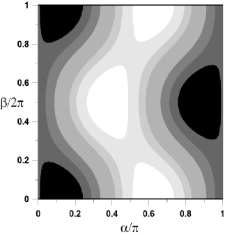
Figure 1: The asymptotic probability $\Pi_{L}$ as a function of dimensionless angles using Eq. (21). Seven zones of probability are given with different tonalities of gray. From the black to the white zone the intervals of probability are: (1) $\left[0.29,0.34\right]$, (2) $\left[0.34,0.39\right]$, (3) $\left[0.39,0.45\right]$, (4) $\left[0.45,0.52\right]$, (5) $\left[0.52,0.60\right]$, (6) $\left[0.60,0.65\right]$, (7) $\left[0.65,0.71\right]$. In section IV this figure also represents Alice’s strategic space for the game with one measurement

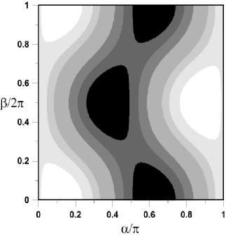
Figure 2: The asymptotic probability $\Pi_{R}$ as a function of dimensionless angles using Eq. (21). Seven zones of probability are given with different tonalities of gray. From the black to the white zone the intervals of probability are: (1) $\left[0.29,0.34\right]$, (2) $\left[0.34,0.39\right]$, (3) $\left[0.39,0.45\right]$, (4) $\left[0.45,0.52\right]$, (5) $\left[0.52,0.60\right]$, (6) $\left[0.60,0.65\right]$, (7) $\left[0.65,0.71\right]$. In section IV this figure also represents Bob’s strategic space for the game with one measurement.

III Periodic measurements in the chirality

In this section we will consider a succession of unitary evolutions of the QW followed by a process of chirality-and-position measurement. Let us take the origin as the initial position of the random walker with the initial condition $|\Psi(0)\rangle$ of Eq. (19). The position and chirality of the walker are jointly measured every $T$ steps, with $T$ sufficiently large in order to use the asymptotic results for the chirality Eq. (21), i.e. $T\sim 2000$. The measurement of any observable of the system produces the collapse of the wave function into an eigenstate of the measured operator. Among the several alternatives for measuring chirality, we choose to measure it in such a way that the chirality is projected on the ${z}$ direction by the Pauli operator $\sigma_{z}$, whose eigenstates are the qubit states $|L\rangle=\binom{1}{0}$ and $|R\rangle=\binom{0}{1}$. The final position can be any position between $k=-T$ and $k=T$ but of course with different probabilities. Due to the fact that we are interested in the time-evolution of the chirality, we can rename the final position measured as the new position $|0\rangle$, this translation does not modify the chirality evolution because this QW is homogeneous in position. Immediately after the measurement has been performed, the system is in state $|L\rangle|0\rangle$ or $|R\rangle|0\rangle$ with probability $\Pi_{L}$ or $\Pi_{R}$ respectively.

The system evolves again unitarily during $T$ time steps and then a second measurement is performed. Let us analyze this second evolution carefully. Supposing first that the system starts from the chirality state $|L\rangle$, after $T$ time steps the new GCD is determined using Eq. (21) with $\alpha=0$, and the value obtained is $\binom{p}{q}$. If instead we start from the chirality state $|R\rangle$ once again using Eq. (21) now with $\alpha=\pi/2$, we obtain a GCD given by $\binom{q}{p}$. In the general case, we have a probability $\Pi_{L}$ of starting from the state $|L\rangle$ and $\Pi_{R}$ of starting from the state $|R\rangle$, therefore we must weigh the previous cases by their probability of occurrence. We obtain in this way the composite probability expression for the GCD after the second measurement

$${\left[\begin{array}[]{c}P_{L}(2T)\\ P_{R}(2T)\end{array}\right]}={\left(\begin{array}[]{cc}p&q\\ q&p\end{array}\right)}\left[\begin{array}[]{c}P_{L}(T)\\ P_{R}(T)\end{array}\right],$$ (22)

where

$${p} =1-\frac{1}{2\sqrt{2}},$$ (23)

$${q} =\frac{1}{2\sqrt{2}},$$ (24)

and we define $P_{L}(T)\equiv\Pi_{L}$ and $P_{R}(T)\equiv\Pi_{R}$.

Eq. (22) is clearly a master equation and the global evolution of the system is a Markov process consisting of a succession of unitary evolutions followed by measurements. Such processes have the property that for any set of successive times ($T,2T,3T,...,mT$) the conditional probability at $mT$ is uniquely determined by the value of stochastic variables at $(m-1)T$ and is not affected by any knowledge of the values at earlier times. In other words, the future state of the system depends only on the current state and not on the path of the process. In our case the measurement of the state of the system is a simple but extreme way of introducing decoherence that produces a loss of long-range memory. After performing $m\geq 2$ measurements the master equation becomes

$${\left[\begin{array}[]{c}P_{L}(mT)\\ P_{R}(mT)\end{array}\right]}={\left(\begin{array}[]{cc}p&q\\ q&p\end{array}\right)}\left[\begin{array}[]{c}P_{L}((m-1)T)\\ P_{R}((m-1)T)\end{array}\right],$$ (25)

and the probabilities as functions of the initial GCD evolution are

$${\left[\begin{array}[]{c}P_{L}(mT)\\ P_{R}(mT)\end{array}\right]}={\left(\begin{array}[]{cc}p&q\\ q&p\end{array}\right)^{m-1}}\left[\begin{array}[]{c}\Pi_{L}\\ \Pi_{R}\end{array}\right],$$ (26)

where $\Pi_{L}$ and $\Pi_{R}$ are given by Eq. (21). After some simple algebra, involving the calculation of the eigenvalues of the previous matrix in Eq. (25), the general solution of Eq. (26) is obtained

$$\left[\begin{array}[]{c}P_{L}(mT)\\ P_{R}(mT)\end{array}\right]=\left(\begin{array}[]{cc}p_{m}&q_{m}\\ q_{m}&p_{m}\end{array}\right)\left[\begin{array}[]{c}\Pi_{L}\\ \Pi_{R}\end{array}\right],$$ (27)

where

$$p_{m} =\frac{1}{2}\left\{1+\left(2p-1\right)^{m-1}\right\},$$

$$q_{m} =\frac{1}{2}\left\{1-\left(1-2q\right)^{m-1}\right\}.$$ (28)

In summary the global evolution of the system, throughout a time interval involving many measurement events, satisfies a master equation and therefore can be described as a Markovian process. The system has an unitary evolution only between consecutive measurements. For a sufficiently large number of measurements, Eq. (27) implies that both $P_{L}$ and $P_{R}$, at first sight, tend to $1/2$ independently of the initial conditions. In order to show this behavior graphically we present Fig. 3 where $P_{R}(2T)$ is calculated using the same color code used in Fig. 2. The values of $P_{R}(2T)$ are approximately restricted to the interval $\left[0.39,0.60\right]$. This shows that the interval of probability $\left[0.45,0.52\right]$ has increased in comparison to the case described by Figs. 1 and 2. Additionally, we also calculated the probabilities when three measurements are performed, that is $P_{R}(3T)$ with $m=3$ in Eq. (27). We verified that $P_{R}(3T)$ is approximately restricted to the interval $\left[0.45,0.52\right]$, meaning that if we used once again the color code adopted before, the corresponding figure would be an uniformly gray square not worthwhile presenting.

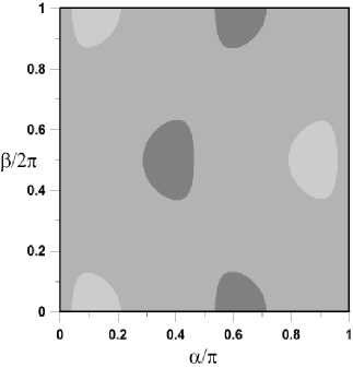
Figure 3: The asymptotic probability $P_{R}(2T)$ as a function of dimensionless angles using Eq. (27) with $m=2$. Three zones of probability are given with different tonalities of gray. From the darker to the lighter zone the intervals of probability are: (1) $\left[0.39,0.45\right]$, (2) $\left[0.45,0.52\right]$, (3) $\left[0.52,0.60\right]$. In section IV this figure also represents Bob’s strategic space for the game with two measurement.

IV Coin-flipping games

Game theory has been used to explore the nature of quantum information. Initially quantum games were proposed as a quantum generalization of their classical counterparts but, due to the principles of quantum mechanics, new game possibilities have arisen within this scenario Meyer ; game1Romanelli ; zabaleta . In the frame of the previous section, let us consider a simple quantum state flip game played between Alice and Bob. Initially the system is prepared in the arbitrary state $|\Psi(0)\rangle$ as in Eq. (19) where $\alpha$ is chosen by Alice and $\beta$ is chosen by Bob, or vice versa. Next the QW dynamics evolves with Eq. (1) up to the time $t\geq T$. At that time the chirality of the system is measured. The players agree that the result of the measurement determines who wins the game. For example, if the state is $|L\rangle$ Alice wins $\$1$ (Bob loses $\$1$) and if the state is $|R\rangle$ Bob wins $\$1$ (Alice loses $\$1$). This is a two-person, zero-sum game; the payoff given to Alice is the exact opposite of that awarded to Bob. If we suppose rational players, the election of their strategies is determined by the election of the initial condition for $|\Psi(0)\rangle$. From Figs. 1 and 2, which show the dependence of probabilities $\Pi_{L}$ and $\Pi_{R}$ with $\alpha$ and $\beta$, we can conclude that the first player to select one of the initial conditions has an advantage. For example, if Alice chooses first, she needs to choose $\alpha\in(0.45\pi,0.55\pi)$ (see Fig. 1) because in this way, independently of what Bob chooses, she makes sure that the probability to obtain $|L\rangle$ is $0.60\leq\Pi_{L}\leq 0.65$ in which case Bob almost certainly loses. On the contrary, if Bob chooses first (see Fig. 2) he needs to choose $\alpha\in(0,0.1\pi)$ or $\alpha\in(0.9\pi,\pi)$ to obtain a probability $0.60\leq\Pi_{R}\leq 0.71$ independently of $\beta$. Therefore, the players must make their measurements obeying the rules of quantum mechanics and the initial conditions of the wave function determines their strategies. By looking at Figs. 1 and 2, the players can plan their strategies and quickly conclude that this is not an equitable game; the first player has many winning strategies.

A possible variant of the previous game is obtained when a second measurement at $t\geq 2T$ is incorporated. In this new game, after the first measurement at $t=T$, the system has an unitary evolution until a second measurement is performed. Once again, Alice wins $\$1$ and Bob loses $\$1$ if the result of the last measurement is $|L\rangle$, independently of the result of the previous measurements. If the last measurement yields $|R\rangle$ Bob wins $\$1$ and Alice loses $\$1$. Fig. 3, shows the probability $P_{R}(2T)$ as a function of the initial conditions $\alpha$ and $\beta$ for the new game. In this figure a large new area with probability $0.45\leq P_{R}(2T)\leq 0.52$ appears. This area shows that this game is fairer because now the initial condition $\beta$ can be chosen in order to balance the $P_{L}(2T)$ and $P_{R}(2T)$ probabilities. If the number of measurements between unitary evolutions is increased, we obtain a succession of more equitable games and in the infinite limit we have a fair game where $P_{L}(\rightarrow\infty)=P_{R}(\rightarrow\infty)=1/2$ for all initial conditions.

Taking into account the inequity of the previous games, the players decide as a strategy to choose $\alpha$ and $\beta$ at random, but obeying the constraint on $|\Psi(0)\rangle$ given by Eq. (19). With the aim to quantify the inequity of these games we now introduce the mean payoff of the game for each player. In the first game using Eq. (21) we can reinterpret $\Pi_{L}$ and $\Pi_{R}$ as the win density for Alice $\sigma_{A}\equiv\Pi_{L}$ and Bob $\sigma_{B}\equiv\Pi_{R}$ as functions of the parameters $\alpha$ and $\beta$. Then the probabilities of winning the game are

$$\pi_{A} \equiv\frac{1}{2}\int\limits_{0}^{2\pi}{d\beta}\int\limits_{0}^{\pi}\sigma_{A}(\alpha,\beta)\text{ }{d\alpha}=1/2$$ (29)

$$\pi_{B} \equiv\frac{1}{2}\int\limits_{0}^{2\pi}{d\beta}\int\limits_{0}^{\pi}\sigma_{B}(\alpha,\beta)\text{ }{d\alpha=}1-\pi_{A}=1/2,$$ (30)

for Alice and Bob respectively. The expected payoff for Alice is $\overset{\_}{\pi}_{A}\equiv\$1\pi_{A}-\$1\pi_{B}$ and the expected payoff for Bob is $\overset{\_}{\pi}_{B}\equiv\$1\pi_{B}-\$1\pi_{A}$; in this game $\overset{\_}{\pi}_{A}=\overset{\_}{\pi}_{B}=\$0$. In the other games, we define the win densities as in the first game but now using Eq. (27)

$$\sigma_{A} =\left[1+\left(2p-1\right)^{m-1}\right]\frac{\Pi_{L}}{2}+\left[1-\left(1-2q\right)^{m-1}\right]\frac{\Pi_{R}}{2},$$

$$\sigma_{B} =\left[1-\left(1-2q\right)^{m-1}\right]\frac{\Pi_{L}}{2}+\left[1+\left(2p-1\right)^{m-1}\right]\frac{\Pi_{R}}{2},$$ (31)

with $m=2,3,4,...$.

The probabilities of winning the game are calculated using Eq. (31) in Eqs.(29, 30). Their values are $\pi_{A}=1/2$, $\pi_{B}=1/2$ again and the expected payoffs for Alice and Bob are $\overset{\_}{\pi}_{A}=\overset{\_}{\pi}_{B}=\$0$. Therefore, it is expected that they will tie on average after many games are played, provided they choose initial conditions at random.

V GCD dynamics with broken links

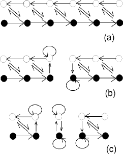
Figure 4: Situations that can arise at a site $k$ of the line when there are: (a) no broken links (Eq. (3)), (b) one link is broken (Eqs.(32,33)), and (c) both continuous links are broken (Eq. (34)). The upper white (lower black) circles indicate the left (right) chirality amplitude. The arrows indicate the direction of the probability flux in one time step. At each circle two arrows point in and two point out in order to conserve the total probability flux.

Let us now consider the breaking of links as a mechanism to introduce decoherence in the QW kendon2010 . This model was presented for the first time in Ref alejo4 . Suppose that, at time $t$, a given site $k$ may have one or both of the links connecting it to its neighboring sites broken. If site $k$ has no broken links, as shown in Fig. 4 $a$, then the evolution law Eq. (3) is applied. When one or both links at site $k$ are opened there can be no translation across the broken link and the evolution must be modified accordingly. If the link to the left of site $k$ is broken, as shown in Fig. 4 $b$, the upper component of the chirality at $k$ receives probability flux from $k+1$. In order to preserve the flux, the outgoing probability flux from the upper component at $k$ must be diverted to the lower component at the same site. The corresponding transformation on the chirality components is therefore

$$a_{k}(t+1) =a_{k+1}(t)\,\cos\theta\,+b_{k+1}(t)\,\sin\theta,\,$$

$$b_{k}(t+1) =a_{k}(t)\,\sin\theta\,+b_{k}(t)\,\cos\theta.$$ (32)

If the broken link is to the right of $k$, the situation is similar and the transformation is

$$a_{k}(t+1) =a_{k}(t)\,\cos\theta\,-b_{k}(t)\,\sin\theta,\,$$

$$b_{k}(t+1) =a_{k-1}(t)\,\sin\theta\,-b_{k-1}(t)\,\cos\theta.$$ (33)

Finally, if site $k$ is isolated, as in Fig. 4 $c$, the unitary operation is followed by a chirality exchange,

$$a_{k}(t+1) =a_{k}(t)\,\cos\theta\,-b_{k}(t)\,\sin\theta,\,$$

$$b_{k}(t+1) =a_{k}(t)\,\sin\theta\,+b_{k}(t)\,\cos\theta.$$ (34)

Hence, there are four situations that can arise at a site $k$: (a) no link is broken, (b) the link on the left side is broken, (c) the link on the right side is broken, and (d) both links are broken. The global evolution of the system depends on the application of one of the four maps in each spatial position, where each map has associated its correlative operator. Thus the dynamical evolution of the GCD can be characterized by four unitary operators which will be called in generic terms $U_{n}$ with $n=0,1,2,3$ where $U_{0}$ will be related to the operator $U$ of Eq. (1). A statistical description can be obtained combining the operators into a single evolution equation with the appropriate statistical weights.

To implement the algorithm of the quantum walk with broken links we proceed as follows. At each time step $t$, the state of the links in the line is defined. Each link has a probability $r$ of breaking in a given time step, being $r$ the only parameter in the model. Therefore the probability that a given site has no adjacent broken link is

$$r_{0}=(1-r)^{2},$$ (35)

that it has a left or right broken link is

$$r_{1}=r_{2}=r(1-r),$$ (36)

and that it is isolated is

$$r_{3}=r^{2}.$$ (37)

These probabilities are appropriate statistical weights since they satisfy

$$r_{0}+r_{1}+r_{2}+r_{3}=1.$$ (38)

In order to study the chirality dynamics of the QW we introduce the reduced density operator

$$\rho_{c}=\mathrm{tr}\rho,$$ (39)

where the operator ‘$\mathrm{tr}$’ is the partial trace taken over the positions and $\rho$ is density matrix of the quantum system

$$\rho=|\Psi(t)\rangle\langle\Psi(t)|.$$ (40)

Using the wave function given by Eq. (2) and its normalization properties, the reduced density matrix obtained in Ref. Carneiro is

$$\rho_{c}=\left(\begin{array}[]{cc}P_{L}(t)&Q(t)\\ Q(t)^{\ast}&P_{R}(t)\end{array}\right).$$ (41)

This matrix depends explicitly on the GCD and its time evolution is given by the time evolution of the GCD. The dynamical equation for $\rho_{c}(t)$ is obtained using the density matrix formalism Kraus ; Brun ; Romanelli09k

$$\rho_{c}(t+1)=\sum_{n=0}^{3}A_{n}\rho_{c}(t)A_{n}^{{\dagger}},$$ (42)

where a set of Kraus operators ($\{{A_{n}}\}$ with $n=0,1,2,3$) has been introduced in order to simulate the decoherence produced by the broken-links process. The Kraus operators are defined by

$${A_{n}\equiv\sqrt{r_{n}}U_{n}},$$ (43)

and, to preserve the trace of the density matrix, they satisfy

$$\sum_{n=1}^{N}A_{n}A_{n}^{{\dagger}}=I,$$ (44)

where $I$ is the identity matrix.

We want to study the quantum evolution of Eq. (42), but this task is not trivial since we do not know the set of operators $\{{A_{n}}\}$ explicitly. However, we can infer some knowledge about the quantum evolution of the GCD if we follow the procedure developed in section $II$ to obtain Eqs. (15) from Eq. (3). Starting from the maps Eqs.(3,32,33,34) the corresponding dynamical equations for the GCD are built. Next these equations are weighted with the probabilities $r_{n}$ to finally obtain the master equation for the averaged GCD

$${\left[\begin{array}[]{c}P_{L}(t+1)\\ P_{R}(t+1)\end{array}\right]} ={\left(\begin{array}[]{cc}\cos^{2}\theta&\sin^{2}\theta\\ \sin^{2}\theta&\cos^{2}\theta\end{array}\right)}\left[\begin{array}[]{c}P_{L}(t)\\ P_{R}(t)\end{array}\right].$$ (51)

This equation has no dependence with the parameter $r$ and, in opposition to Eq. (15), has a negligible interference term $Q(t)$ due to the random phases introduced by the lack of coherence between the terms of the sum that define the interference in Eq. (16). Therefore, if $Q(t)$ is negligible it is clear that Eq. ( 42) is equivalent to Eq. (51), and we could use this equivalence to obtain information about the operators $\{{A_{n}}\}$.

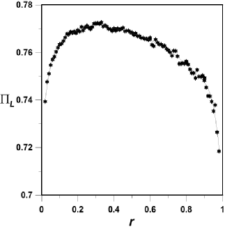
Figure 5: The asymptotic probability $\Pi_{L}$ as a function of the probability $r$ with $\theta=\pi/4$ and the initial condition $\frac{1}{\sqrt{2}}\binom{1}{1}$. The stars are the values obtained from the numerical calculation and the thin line is a polynomial adjustment. The calculation has been made using the map Eq. (3) for the left side of the evolution and the maps Eqs. (3,32,33,34) weighted with the values given by Eqs. (35,36,37) for the right side of the evolution.

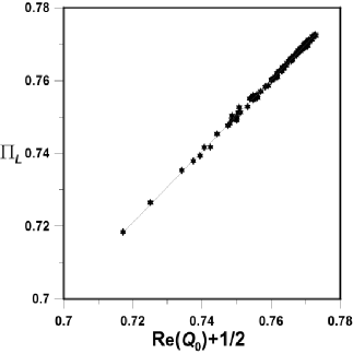
Figure 6: The asymptotic probability $\Pi_{L}$ as a function of the dimensionless term Re$(Q_{0})+1/2$, with $\theta=\pi/4$ (see Eq. (18)) and the initial condition $\frac{1}{\sqrt{2}}\binom{1}{1}$. The stars are the values obtained from the numerical calculation and the thin line is a linear adjustment with slope $1$. The calculation has been made using the map Eq. (3) for the left side of the evolution and the maps Eqs. (3,32,33,34) weighted with the values given by Eqs. (35,36,37) for the right side of the evolution.

The stationary solution of Eq. (51) is $\Pi_{L}=\Pi_{R}=1/2$ independently of the initial conditions and of $\theta$. We implemented a numerical code with the four maps Eqs. (3,32,33,34), weighted with the values $r_{0}$, $r_{1}$, $r_{2}$, $r_{3}$ respectively, and have verified the asymptotic value $\Pi_{L}=1/2$ for several initial conditions and several values of $\theta$ and $r$. Thus, the theoretical result given by Eq. (51) has been numerically confirmed.

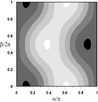
Figure 7: The asymptotic probability $\Pi_{L}$ as a function of dimensionless angles. The calculation has been made using the map Eq. (3) for the left side of the evolution and the maps Eqs. (3,32,33,34) weighted with the values given by Eqs. (35,36,37) for the right side of the evolution, with $r=0.3$. Seven zones of probability are given with different tonalities of gray, from the black to the white zone the intervals of probability are: (1) $\left[0.738,0.746\right]$, (2) $\left[0.746,0.755\right]$, (3) $\left[0.755,0.763\right]$, (4) $\left[0.763,0.771\right]$, (5) $\left[0.771,0.780\right]$, (6) $\left[0.780,0.789\right]$, (7) $\left[0.789,0.797\right]$.

The usual QW dynamics, Eq. (3), has the property of spreading over the line quadratically faster than its classical analog and after a long time its wave-function is very dispersed on the line. This situation makes it interesting to study the decoherence when only some segment on the line is affected by the breakage of links. Such decoherence mechanisms may be relevant as a model of experimental realizations in quantum computation Exp ; ProExp ; Berman as well as in any problem related to the transfer of quantum information through space using QW childs ; Lovett . In order to investigate this type of decoherence, we propose a composed non-homogeneous QW with two different dynamics starting form the origin: for the left half-line the evolution is determined by Eq. (3) and for the right half-line it is determined by the set of equations Eqs. (3,32,33,34), weighted with the values $r_{0}$, $r_{1}$, $r_{2}$, $r_{3}$ respectively. The stochastic behavior of the GCD , for an ensemble of these QWs, will depend, for the left side, on the usual QW and, for the right side, on the QW with broken links. Therefore the right half-line chirality distribution satisfies Eq. (51) and the left half-line chirality distribution satisfies Eq. (15). From this reasoning, it is clear that the GCD is the sum of the above right and left partial distributions and it satisfies Eq. (15), where the interference term emerges from the amplitudes of the wave function belonging to the left side of the evolution. However, it should be noted that the incorporation of the interference term of the right side of the evolution does not modify this equation because it remains negligible.

The evolution of the system ceases to be unitary owing to decoherence, however in spite of the stochastic nature of the system Re$(Q_{0})\neq 0$ and Eq. (18) maintains the dependence between the asymptotic values $\Pi_{L}$ and Re$(Q_{0})$. The system loses its integrability and the explicit value of $\Pi_{L}$ is to be calculated numerically. We have performed this calculation, as a function of the probability $r$ with $\theta=\pi/4$ using the original maps Eqs. (3,32,33,34) with an ensemble of $100$ dynamical trajectories and $2000$ time steps. Figure 5 shows that $\Pi_{L}$ has a parameter dependence on $r$. Figure 6 shows the linear dependence between $\Pi_{L}$ and Re$(Q_{0})+1/2$, with slope $1$ for $\theta=\pi/4$, verifying the stationary solution given by Eq. (18). Therefore, we conclude that there is a perfect agreement between the theoretical stochastic approach presented in this section and the numerical calculation using the original maps. We also found from the numerical calculation that the asymptotic distribution $\Pi_{L}$ depends on the initial conditions. Figure 7 presents the numerical calculation of the distribution $\Pi_{L}$, with $3000$ time steps and the initial condition given by Eq. (19).

Comparing Fig. 7 with Fig. 1, it is possible to distinguish several similarities, such as the number of light and dark spots in both figures. These similarities, show that the asymptotic behavior depends on the initial condition. In other words, this type of decoherence erases the unitary behavior of the system but does not completely erase its dependence on the initial condition. However, the range of values of the probability is now restricted to $\sim\left[0.7,0.8\right]$ while in the Fig. 1 this range was $\sim\left[0.3,0.7\right]$. Such a decrease in the range shows that the trend of the system is to go to a single asymptotic distribution that will only depend on the parameter $r$, as seen in Fig. 5.

VI Conclusions

Decoherence in quantum systems like the QW has been extensively studied. Analytical and numerical results on the effect of different kinds of noise have shown that quantum properties are highly sensitive to random events. In this paper, we studied the asymptotic behavior of the QW on the line when it is subjected to different sources of decoherence. We focused on the dynamics of the GCD when decoherence is introduced in two different ways. In the first case decoherence is introduced through periodic measurements of position and chirality. It has been shown that the evolution of the GCD, in a time scale involving many measurements, can be described as a Markovian process and its master equation has been obtained analytically. This master equation allows us to build new quantum games, similar to the usual spin-flip game, where as a novelty the players perform measurements on the QW system. These games are characterized by a continuous space of strategies, and the selection of an initial condition determines the particular strategy chosen by the player. These games may be used as a tool to study quantum algorithms subjected to external decoherence, as in the extreme case of measurement.

In the second case, the decoherence is introduced through the influence of randomly broken links affecting the QW dynamics. Two different variants of this second case have been investigated. These are: (a) All the QW links have a certain probability of being broken, the GCD is described by a Markovian process. Its master equation is obtained analytically and it is shown to be equivalent to the dynamical equation of the density matrix. It was shown that the dynamics is independent both of the breakage probability and of the coin bias of the QW. (b) Only the links on one of the half-lines (say the right one) are affected by the possibility of breakage. In this case the dynamical evolution of the GCD is not described by a Markovian process but it has an asymptotic value that depends on the initial conditions and the breakage probability. Here the interference term $Q_{0}$ is not negligible but an asymptotic stationary relation between $Q_{0}$ and the GCD has been analytically found. The behavior of this composite QW is at first sight unexpected since usually decoherence destroys the unitary correlation, providing a route towards a classical-like behavior described by a Markov process. To understand this behavior suppose a localized initial condition far to the left of the origin, situated thus in a zone where the evolution is determined by the usual QW map. As time passes, the wave function spreads in both directions and, due to the dynamical evolution of the map, the extreme left branch of the wave function will never be influenced by the existence of decoherence introduced into the right branch of the wave function. In this way, the wave function keeps some information about the initial condition. We conclude that the effect of decoherence of the second kind studied in this work does not necessarily transform the quantum system into a dissipative one such as a Markov process. In more general terms, the mere presence of noise does not assure the transition of a quantum system to classicality.

We acknowledge the comments made by V. Micenmacher and the support from PEDECIBA and ANII.

References

- (1) P.W. Shor, in: Proc. of the 35th Annual Symposium on the Foundations of Computer Science, Ed. S. Goldwasser, (Los Alamitos, CA, 1994), SIAM J. Comp., 26, 1484, (1997).
- (2) L.K. Grover, in: Proc. 28th STOC, 212, Philadelphia, PA (1996); L.K. Grover, Phys. Rev. Lett. 79,325 (1997) M. Nielssen and I. Chuang, Quantum Computation and Quantum Information, (Cambridge University Press, 2000).
- (3) Y. Aharonov, L. Davidovich, and N. Zagury, Phys. Rev. A 48, 1687 (1993); D. A. Meyer, J. Stat. Phys. 85, 551 (1996); J. Watrous, Proc. STOC’01 (ACM Press, New York, 2001), p.60; A. Ambainis, Int. J. Quant. Inf. 1, 507 (2003); J. Kempe, Contemp. Phys. 44, 307 (2003); V. Kendon, Math. Struct. Comp. Sci. 17, 1169 (2006); V. Kendon, Phil. Trans. R. Soc. A 364, 3407 (2006); N. Konno, in Quantum Potential Theory, Lect. Notes Math., Vol. 1954, edited by U. Franz and M. Schürmann (Springer, 2008).
- (4) A.M. Childs, Phys. Rev. Lett. 102, 180501 (2009).
- (5) A. Romanelli, Phys. Rev. A, 80, 042332 (2009).
- (6) N. Linden, and J. Sharam, Phys. Rev. A, 80, 052327 (2009).
- (7) A. Childs, E. Deotto, E. Farhi, S. Gutmann, and D. A. Spielman, in Proc. 35th ACM Symposium on Theory of Computing (STOC 2003), pp. 59–68, 2003.
- (8) N. Shenvi, J. Kempe, K. BirgittaWhaley, Phys. Rev. A 67, 052307 (2003).
- (9) N.B. Lovett, S. Cooper, M. Everitt, M. Trevers, and V. Kendon, Phys. Rev. A 81, 042330 (2010).
- (10) H.B. Perets et al., Phys. Rev. Lett. 100, 170506 (2008). A. Schreiber et al., Phys. Rev. Lett. 104, 050502 (2010). M. Karski, L. Förster, Jai-Min Choi, A. Steffen, W. Alt, D. Meschede, A. Widera, Science 325, 174 (2009). M.A. Broome, A. Fedrizzi, B.P. Lanyon, I. Kassal, A. Aspuru-Guzik, and A.G. White, Phys. Rev. Lett. 104, 153602 (2010)
- (11) W. Dür, R. Raussendorf, V.M. Kendon, and H.J. Briegel, Phys. Rev. A 66, 052319, (2002). B.C. Travaglione and G.J. Milburn, Phys. Rev. A 65, 032310, (2002). B.C. Sanders, S.D. Bartlett, B. Tregenna, and P.L. Knight, Phys. Rev. A 67, 042305 (2003). P.L. Knight, E. Roldán, and J.E. Sipe, Phys. Rev. A 68, 020301(R) (2003); Opt. Commun. 227, 147 (2003); erratum 232, 443 (2004); J. Mod. Opt. 51, 1761 (2004). D. Bouwmeester, I. Marzoli, G.P. Karman, W. Schleich, and J.P. Woerdman, Phys. Rev. A 61, 013410 (1999). B. Do et al., J. Opt. Soc. Am. B 22, 499 (2005). C. M. Chandrashekar, Phys. Rev. A 74, 032307 (2006).
- (12) B. Tregenna, W. Flanagan, R. Maile, and V. Kendon, New J. Phys. 5 83 (2003). V. Kendon and B. Tregenna, Phys. Rev. A 67, 042315 (2003). T. A. Brun, H. A. Carteret and A. Ambainis, Phys. Rev. A 67, 052317 (2003). A. Wójcik, T. Luczak, P. Kurzynski, A. Grudka, and M. Bednarska, Phys. Rev. Lett. 93, 180601 (2004). A. Romanelli, A. Auyuanet, R. Siri, G. Abal, and R. Donangelo. Physica A, 352, 409 (2005). M. C. Bañuls, C. Navarrete, A. Pérez, E. Roldán, and J. C. Soriano, Phys. Rev. A 73, 062304 (2006). C. Navarrete-Benlloch, A. Pérez, and E. Roldán, Phys. Rev. A 75, 062333 (2007). P. Ribeiro, P. Milman, and R. Mosseri, Phys. Rev. Lett. 93, 190503 (2004).
- (13) A. Romanelli, R. Siri, G. Abal, A. Auyuanet, and R. Donangelo, Physica A, 347, 137 (2005).
- (14) A. Romanelli, A. Auyuanet, R. Donangelo, Physica A, 375 133 (2007).
- (15) T. A. Brun, H. A. Carteret and A. Ambainis, Phys. Rev. A 67, 032304 (2003).
- (16) T. A. Brun, H. A. Carteret and A. Ambainis, Phys. Rev. Lett. 91, 130602 (2003).
- (17) A. Romanelli, Phys. Rev. A 76, 054306 (2007). A. Romanelli, Phys. Rev. A 80, 022102 (2009). H. Schomerus and E. Lutz, Phys. Rev. Lett. 98, 260401 (2007). H. Schomerus and E. Lutz, Phys. Rev. A 77, 062113 (2008). A. Romanelli, A. Auyuanet, R. Siri and V. Micenmacher. Phys. Lett. A, 365, 200 (2007). A. Romanelli, R. Siri, V. Micenmacher. Phys. Rev. E 76, 037202 (2007). A. Romanelli. Phys. Rev. E 78, 056209 (2008).
- (18) A. Romanelli, Phys. Rev. A, 81, 062349 (2010).
- (19) D.A. Meyer, Phys. Rev. Lett. 82, 1052 (1999). S. J. van Enk, Phys. Rev. Lett. 84, 789 (2000). D.A. Meyer, Phys. Rev. Lett. 84, 790 (2000).
- (20) A. Romanelli, Physica A, 379 545 (2007).
- (21) O.G. Zabaleta, C.M. Arizmendi, Physica A, 389 2858 (2010).
- (22) G.P. Berman, D.I. Kamenev, R.B. Kassman, C. Pineda, V.I. Tsifrinovich, Int. J. Quant. Inf. 1 51 (2003).
- (23) A. Romanelli, A.C. Sicardi Schifino, G. Abal, R. Siri, and R. Donangelo, Phys. Lett. A 313, 325 (2003).
- (24) A. Romanelli, A.C. Sicardi Schifino, R. Siri, G. Abal, A. Auyuanet, and R. Donangelo, Physica A, 338, 395 (2004).
- (25) G. Abal, R. Siri, A. Romanelli, and R. Donangelo, Phys. Rev.A 73, 042302, 069905(E) (2006).
- (26) 10 A. Nayak and A. Vishwanath, e-print quant-ph/0010117
- (27) D.R. Cox and H.D. Miller, The theory of stochastic processes, (Chapman and Hall, London, 1978).
- (28) G. Leung, P. Knott, J.Bailey, and V. Kendon, arXiv:1006.1283v1 (2010). M. Annabestani, and S. J. Akhtarshenas, arXiv:0910.1986v1 (2009). M. Sawerwain, and R. Gielerak, arXiv:1003.3779v1 (2010).
- (29) I. Carneiro, M. Loo, X. Xu, M. Girerd, V. M. Kendon, and P. L. Knight, New J. Phys. 7, 56 (2005).
- (30) K. Kraus, States, effects and operations: fundamental notions of quantum theory, (Springer-Verlag, Berlin, 1983).