Feynman’s path-integral polaron treatment approached using time-ordered operator calculus^∗

Abstract

The Feynman all-coupling variational approach for the polaron is re-formulated and extended using the Hamiltonian formalism with time-ordered operator calculus. Special attention is devoted to the excited polaron states. The energy levels and the inverse lifetimes of the excited polaron states are, for the first time, explicitly derived within this all-coupling approach. Remarkable agreement of the obtained transition energies with the peak positions of the polaron optical conductivity calculated using diagrammatic quantum Monte Carlo is obtained.

Several studies have been devoted to the search of a Hamiltonian formalism equivalent to Feynman’s path integral approximation to polaron theory. Bogolubov [2] reproduced the Feynman result for the polaron free energy [3] using time-ordering T-products . Yamazaki [4] introduced two kinds of auxiliary vector fields to derive Feynman’s ground state polaron energy expression with the operator technique, however he found no proof of the variational nature of this result. Cataudella et al. [5] formally re-obtained Feynman’s polaron ground-state energy expression by introducing additional degrees of freedom, but again their result could not be proved to constitute an upper bound for the polaron ground state energy.

The study of the excited polaron states is of interest i. a. for its application to the polaron response properties. In [6] a path-integral based response-formalism was introduced that was applied to derive polaron optical absorption spectra in [7]. The results for the polaron response obtained in [7] were re-derived with a Hamiltonian technique (Mori- formalism) in [8].

To the best of our knowledge, no explicit description of the polaron excited states has been derived within the “all coupling-“ Feynman approach. Only for the limiting cases of weak and strong coupling approximations (and for a 1D-model system) such excitation spectra were derived [9, 10].

In principle, the spectrum of the polaron excited states can be derived indirectly – using a Laplace transform of the finite-temperature partition function. However, it is not clear how to realize this program in practice.

The polaron excitation spectrum is interesting by itself. E.g. the existence and the nature of “relaxed excited states”, “Franck-Condon states”, “scattering states” is understood from the mathematical structure of corresponding eigenstates.

In the present letter we first present a re-derivation of the original Feynman variational path integral polaron model [3] for the ground state, using a Hamiltonian formalism, and we do provide a proof of the upper bound nature of the obtained ground state energy. Furthermore, using Feynman’s (Hamiltonian-) time-ordered operator calculus (and an ad hoc unitary transformation) we obtain explicitly – and for the first time – the excited polaron states that correspond to the Feynman polaron model.

The novelty of the present approach consists (a) in the direct calculation of the energies and the lifetimes of the excited polaron states (within a Hamiltonian all-coupling approach – developed in this work – equivalent to the Feynman path integral polaron model) and (b) in the extension of the Feynman variational technique to non-parabolic trial potentials. Although the time-ordered operator calculus is formally equivalent to the path-integral formalism, it is not obvious how to directly calculate the excited polaron states using path integrals.

The present work, formulated with the (Hamiltonian) time ordered operator calculus, thus provides an (equivalent) tool complementary with respect to the Feynman path integral approach to the polaron, to study the polaron problem. Additionally we directly study the excited polaron states.

Consider an electron-phonon system with the Fröhlich Hamiltonian

$$H =\frac{\mathbf{p}^{2}}{2}+H_{ph}+H_{e-ph},$$ (1)

$$H_{ph} =\sum_{\mathbf{q}}\left(a_{\mathbf{q}}^{+}a_{\mathbf{q}}+\frac{1}{2}\right),$$ (2)

$$H_{e-ph} =\frac{1}{\sqrt{V}}\sum_{\mathbf{q}}\frac{\sqrt{2\sqrt{2}\pi\alpha}}{q}\left(a_{\mathbf{q}}+a_{-\mathbf{q}}^{+}\right)e^{i\mathbf{q\cdot r}}.$$ (3)

Here, the Feynman units are used: $\hbar=1,$ the band mass $m_{b}=1,$ the LO-phonon frequency $\omega_{\mathrm{LO}}=1$.

The polaron partition function after exact averaging over phonon states is

$$Z_{pol}=\mathtt{Tr}\left[\mathtt{T}\exp\left(-\int_{0}^{\beta}\frac{\mathbf{p}_{\tau}^{2}}{2}d\tau+\hat{\Phi}\left[\mathbf{r}_{\tau}\right]\right)\right],$$ (4)

where $\beta=\frac{1}{k_{B}T}$. The “influence phase” of the phonons $\hat{\Phi}\left[\mathbf{r}_{\tau}\right]$ in the the time-ordered operator calculus has the same form as in the path-integral representation. The polaron free energy is determined as

$$F_{pol}=-\frac{1}{\beta}\ln Z_{pol}.$$ (5)

The trial Hamiltonian describes the electron interacting with a fictitious particle of the mass $m_{f}$ through an attractive potential $V_{f}$:

$$H_{tr}=\frac{\mathbf{p}^{2}}{2}+\frac{\mathbf{p}_{f}^{2}}{2m_{f}}+V_{f}\left(\mathbf{r}-\mathbf{r}_{f}\right).$$ (6)

The trial potential $V_{f}$ is, in general, non-parabolic. The parabolic potential with frequency parameter $w$ corresponds to the Feynman polaron model.

Consider the “extended” partition function of the electron-phonon system

$$Z_{ext}=Z_{f}Z_{pol}$$ (7)

where $Z_{f}$ is the partition function of a fictitious particle,

$$Z_{f}\equiv\mathtt{Tr}\left[\mathtt{T}\exp\left(-\int_{0}^{\beta}d\tau H_{f,\tau}\right)\right],$$ (8)

with Hamiltonian

$$H_{f}=\frac{\mathbf{p}_{f}^{2}}{2m_{f}}+V_{f}\left(\mathbf{r}_{f}\right).$$ (9)

The polaron free energy is expressed as the difference

$$F_{pol}=F_{ext}-F_{f},$$ (10)

where $F_{f}$ is the free energy of the fictitious particle confined to the potential $V\left(\mathbf{r}_{f}\right)$. The free energies $F_{ext}$ and $F_{f}$ are determined similarly to (5), with corresponding partition functions. In the zero-temperature limit, the free energies $F_{pol}$, $F_{ext}$ and $F_{f}$ become, respectively, the ground-state energies $E_{pol}^{0}$, $E_{ext}^{0}$ and $E_{f}^{0}$.

The key element of the present approach is the unitary transformation

$$U=e^{-i\mathbf{p}_{f}\cdot\mathbf{r}}.$$ (11)

Application of this canonical transformation results in the transformed “extended” Hamiltonian $H_{ext}^{\prime}=UH_{ext}U^{-1}$,

$$H_{ext}^{\prime} =\frac{\left(\mathbf{p}+\mathbf{p}_{f}\right)^{2}}{2}+\frac{\mathbf{p}_{f}^{2}}{2m_{f}}+V_{f}\left(\mathbf{r}_{f}-\mathbf{r}\right)$$

$$+H_{ph}+H_{e-ph}.$$ (12)

This Hamiltonian can be represented as a sum of an unperturbed Hamiltonian

$$H_{0}\equiv H_{tr}+H_{ph}$$ (13)

and an interaction term

$$V\equiv\frac{1}{2}\mathbf{p}_{f}^{2}+\mathbf{p}\cdot\mathbf{p}_{f}+H_{e-ph}.$$ (14)

Further we use the variational principle for the ground-state energy in terms of the time-ordered operators following Ref. [11]. The exact ground state $\left|0\right\rangle$ of the system with the Hamiltonian (12) can be written in the interaction representation starting from the unperturbed ground state $\left|-\infty\right\rangle$:

$$\left|0\right\rangle=\mathcal{U}\left(\infty,-\infty\right)\left|-\infty\right\rangle$$ (15)

where $\mathcal{U}\left(\infty,-\infty\right)$ is the time-evolution operator,

$$\mathcal{U}\left(t_{2},t_{1}\right)=\mathcal{T}\exp\left(-i\int_{t_{1}}^{t_{2}}e^{-\delta\left|t\right|}e^{iH_{0}t}Ve^{-iH_{0}t}\right).$$ (16)

Here, $\delta\rightarrow+0$ and $\mathcal{T}$ denotes time ordering.

In the exact expectation value for the ground state energy $E_{ext}^{0}\equiv\left\langle 0\left|H_{ext}^{\prime}\right|0\right\rangle$, the phonons are eliminated using the time ordered-operator calculus as in Ref. [11]. The average of the interaction term becomes then

$$\left\langle 0\left|H_{e-ph}\right|0\right\rangle$$

$$=-i\frac{\sqrt{2}\pi\alpha}{V}\int_{-\infty}^{\infty}dte^{-i\left|t\right|-\delta\left|t\right|}$$

$$\times\sum_{\mathbf{q}}\frac{1}{q^{2}}\left\langle\infty\left|\mathcal{T}\left[\mathcal{U}\left(\infty,-\infty\right)e^{i\mathbf{q}\cdot\left[\mathbf{r}\left(t\right)-\mathbf{r}\left(0\right)\right]}\right]\right|-\infty\right\rangle.$$ (17)

This means that the polaron ground state energy is exactly described using a retarded potential in the interaction representation, cf. Eq. (2.16) of Ref. [11].

The ground state energy satisfies the Ritz variational principle with a trial state. Choosing the trial state as the ground state of the Hamiltonian (13), the variational principle can be written as [11]

$$E_{ext}^{0} \leq E_{tr}^{0}$$

$$+\left\langle\infty\left|\mathcal{T}\left\{\mathcal{U}_{tr}\left(\infty,-\infty\right)\left[H_{ext}^{\prime}\left(0\right)-H_{0}\left(0\right)\right]\right\}\right|-\infty\right\rangle,$$ (18)

where $\mathcal{U}_{tr}\left(\infty,-\infty\right)$ is the time-evolution operator corresponding to the trial Hamiltonian (6).

The exact polaron ground state energy is denoted here as $E^{0}\left(\mathbf{k}\right)$, where $\mathbf{k}$ is the polaron translation momentum. We find an upper bound for $E^{0}\left(\mathbf{k}\right)$ substituting (17) in (18) and using the exact wave functions and energy levels of the trial Hamiltonian. The trial Hamiltonian (6) can be rewritten in terms of the coordinates $\left(\mathbf{R},\boldsymbol{\rho}\right)$ and momenta $\left(\mathbf{P},\vec{\pi}\right)$ of the center-of-mass and relative (internal) motions of the trial system with the masses $M=1+m_{f}$ and $\mu=m_{f}/\left(1+m_{f}\right)$ using the frequency $v=wM$. The energy spectrum of the trial system is the sum of the translation- and oscillation contributions,

$$E_{\mathbf{k},n}=\frac{\mathbf{k}^{2}}{2M}+\varepsilon_{n},\;\varepsilon_{n}=v\left(n+\frac{3}{2}\right).$$ (19)

The eigenfunctions of the Hamiltonian (6) are products of translational- and oscillatory wave functions:

$$\psi_{\mathbf{k};l,n,m}\left(\mathbf{R},\boldsymbol{\rho}\right)=\frac{1}{\sqrt{V}}e^{i\mathbf{k\cdot R}}\varphi_{l,n,m}\left(\boldsymbol{\rho}\right),$$ (20)

where $\varphi_{l,n,m}\left(\boldsymbol{\rho}\right)$ is the 3D harmonic-oscillator wave function with a given angular momentum. The result is

$$E^{0}\left(\mathbf{k}\right) \leq\mathcal{E}_{p}^{\left(0,0\right)}\left(\mathbf{k}\right),$$ (21)

$$\mathcal{E}_{p}^{\left(0,0\right)}\left(\mathbf{k}\right) =\frac{3}{4}\frac{\left(v-w\right)^{2}}{v}$$

$$+\frac{1}{2}\left(1-\frac{1}{\left(1+m_{f}\right)^{2}}\right)\mathbf{k}^{2}-\frac{\sqrt{2}\alpha}{4\pi^{2}}\int\frac{d\mathbf{q}}{q^{2}}$$

$$\times\sum_{\mathbf{k}^{\prime},l^{\prime},n^{\prime},m^{\prime}}\frac{\left|\left\langle\psi_{\mathbf{k};0,0,0}\left|e^{i\mathbf{q\cdot r}}\right|\psi_{\mathbf{k}^{\prime};l^{\prime},n^{\prime},m^{\prime}}\right\rangle\right|^{2}}{\frac{1}{2\left(m_{f}+1\right)}\left(\left(\mathbf{k}^{\prime}\right)^{2}-\mathbf{k}^{2}\right)+vn^{\prime}+1},$$ (22)

where $v>w$ are the Feynman variational frequencies. The functional (22) can be reduced to the known Feynman result for the polaron ground-state energy. In the r.h.s. of (22 at the polaron momentum $\mathbf{k}=0$, we introduce the integral over the Euclidean time:

$$\frac{1}{\frac{\left(\mathbf{k}^{\prime}\right)^{2}}{2\left(m_{f}+1\right)}+vn^{\prime}+1}=\int_{0}^{\infty}e^{-\left(\frac{\left(\mathbf{k}^{\prime}\right)^{2}}{2\left(m_{f}+1\right)}+vn^{\prime}+1\right)\tau}d\tau.$$ (23)

After this, the summations and integrations in (25) are performed analytically, and we arrive at the Feynman variational expression for the polaron ground-state energy:

$$\left.E^{0}\left(\mathbf{k}\right)\right|_{\mathbf{k}=0} \leq\frac{3}{4}\frac{\left(v-w\right)^{2}}{v}$$

$$-\frac{\alpha v}{\sqrt{\pi}}\int_{0}^{\infty}\frac{e^{-\tau}}{\sqrt{w^{2}\tau+\frac{v^{2}-w^{2}}{v}\left(1-e^{-v\tau}\right)}}d\tau.$$ (24)

The electron-phonon contribution in (22) is structurally similar to the second-order perturbation correction to the polaron ground-state energy due to the electron-phonon interaction (using states of the Feynman model $\psi_{\mathbf{k};l,n,m}$ as the zero-order approximation). Therefore we can estimate the energies of the excited polaron states when averaging the difference between exact and unperturbed Hamiltonians in (18) with an excited trial state. We then arrive at the following extension for the r.h.s. of (22):

$$\mathcal{E}_{p}^{\left(l,n\right)}\left(\mathbf{k}\right) =\frac{v^{2}+w^{2}}{2v}\left(n+\frac{3}{2}\right)-\frac{3}{2}w$$

$$+\frac{1}{2}\left(1-\frac{1}{\left(1+m_{f}\right)^{2}}\right)\mathbf{k}^{2}-\frac{\sqrt{2}\alpha}{4\pi^{2}}\int\frac{d\mathbf{q}}{q^{2}}$$

$$\times\sum_{\mathbf{k}^{\prime},l^{\prime},n^{\prime},m^{\prime}}\frac{\left|\left\langle\psi_{\mathbf{k};l,n,m}\left|e^{i\mathbf{q\cdot r}}\right|\psi_{\mathbf{k}^{\prime};l^{\prime},n^{\prime},m^{\prime}}\right\rangle\right|^{2}}{\frac{1}{2\left(m_{f}+1\right)}\left(\left(\mathbf{k}^{\prime}\right)^{2}-\mathbf{k}^{2}\right)+v\left(n^{\prime}-n\right)+1}.$$ (25)

In the same approach, we obtain the inverse lifetimes for the excited states of the polaron:

$$\Gamma_{l,n}\left(\mathbf{k}\right) =\frac{\sqrt{2}\alpha}{4\pi}\sum_{\mathbf{k}^{\prime},l^{\prime},n^{\prime},m^{\prime}}\int d\mathbf{q}\frac{1}{q^{2}}$$

$$\times\left|\left\langle\psi_{\mathbf{k};l,n,m}\left|e^{i\mathbf{q\cdot r}}\right|\psi_{\mathbf{k}^{\prime};l^{\prime},n^{\prime},m^{\prime}}\right\rangle\right|^{2}$$

$$\times\delta\left(\frac{q^{2}}{2\left(m_{f}+1\right)}+v\left(n^{\prime}-n\right)+1\right).$$ (26)

The broadening of the excited polaron “non-scattering” states must be taken into account for an analytical study of the polaron optical conductivity.

Using the above expressions, we determine the transition energies for the transitions between the ground and the first excited state $\hbar\Omega_{0\rightarrow 1exc}\equiv E_{p}^{\left(1exc\right)}-E_{p}^{\left(0\right)}$. Let us first consider the transition energies in which $E_{p}^{\left(1exc\right)}$ are calculated using optimal values of the parameters of the Feynman model obtained from the minimization of the variational ground-state energy $E_{p}^{\left(0\right)}$. This method formally leads to the Franck-Condon (FC) excited states, with the “frozen” phonon configuration corresponding to the ground state of the polaron. Note that the existence of Franck-Condon states as eigenstates of the Fröhlich polaron Hamiltonian has not been proved: Ref [10] suggests their non-existence as eigenstates for a simplified polaron model. Nevertheless the Franck-Condon concept can be significant, e. g. for approximate treatments using a basis of Franck-Condon states, as indicative for the frequency of the maxima of phonon-sidebands, etc.

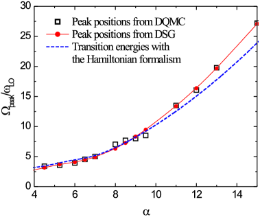
Figure 1: Franck-Condon transition energies as a function of the coupling constant compared to the lowest-energy peak position of the polaron optical conductivity from Ref. [7] and the maximum of the polaron optical conductivity band from Ref. [12].

In Fig. 1, the FC transition energies calculated with the approach introduced in the present work for polaron momentum $\mathbf{k}=0$ are plotted as a function of the coupling constant $\alpha$. They are compared with the peak energies of the polaron optical conductivity calculated using the diagrammatic Monte Carlo method (DQMC) [12, 13] and with the peak energies attributed to polaron “relaxed excited states” (RES) in Ref. [7] (“DSG”). The DQMC and DSG main-peak energies are close to each other in the whole range of the coupling strength. In the range $4\lessapprox\alpha\lessapprox 10$, the present result for the transition energy is close to the DQMC and the DSG peak energies. Furthermore, in this range of $\alpha$, the non-monotonous behavior of the curvature is remarkably the same for the DQMC and DSG peak energies and for the present result.

There is a remarkable agreement between the peaks attributed to the RES in Ref. [7], the peak positions obtained within the strong-coupling approach, Eq. (3) of Ref. [13], and the positions of the maximum of the optical conductivity band calculated in Ref. [12] using DQMC. It is reasonable that the three aforesaid peaks must be interpreted in one and the same way. In order to clarify this, we can refer to Ref. [12]. In the strong-coupling regime, the dominant broad peak of the polaron optical conductivity spectrum can be considered as a “Franck-Condon sideband” of the “groundstate to RES-transition”, even if this latter transition can have a negligible oscillator strength (see also [14]). The optical conductivity spectra of Ref. [13] in the strong-coupling approximation have been calculated taking into account the polaronic shift of the energy levels. The polaronic shift in Ref. [13] has been calculated with the Franck-Condon wave functions (i. e., with the strong-coupling wave functions corresponding to the “frozen” lattice configuration for the ground state). Note that the exact excitation spectrum of the Fröhlich-Hamiltonian might be devoid of Franck-Condon eigenstates, cf. Ref. [10]). It should be remarked that the maxima of the FC-sideband structures of Ref. [7] are positioned at the frequency $\Omega=v$, i. e., at the transition frequency for the model system without the polaron shift.

The Franck-Condon peak energies calculated in the present work also take into account the polaron shift. As follows from the above analysis, in the strong-coupling limit they must correspond to the Franck-Condon peak energies of the strong-coupling expansion of Ref. [13]. The agreement of the position of the maxima of these peaks with those attributed to transitions to the RES in Ref. [7] shows that in the strong-coupling range of $\alpha$, the latter should be associated to the Franck-Condon sidebands rather than to the RES.

Another approach, in which the parameters of the first excited state are determined self-consistently (Ref. [14]), was used i. a. to calculate (in the strong-coupling case) the (lowest) energy level of the relaxed excited state (RES). The transitions from the polaron ground state to the RES correspond to a zero-phonon peak in the optical conductivity.

For the study of the energies of excited states of the polaron, a variational approach requires special care, because the excited states of the polaron are not stable. A variational approach, strictly speaking, is only valid for excited states when the variational wave function of the excited state is orthogonal to the exact ground-state wave function.

For the estimation of the energy of the first RES with our present formalism, we determine a minimum of the expression (25) in a physically reasonable range of the variational parameters. In order to determine that range, we refer to Ref. [15], where the energy of the polaron RES is calculated variationally within the Green’s function formalism.

The expression for the RES energy in Ref. [15] contains the electron-phonon contribution corresponding to the second-order perturbation formula. It differs, however, from the weak-coupling second-order perturbation expression by the choice of the unperturbed states: in Ref.[15] those are variational states rather than free-electron states. There exists some analogy between our approach and that of Ref. [15]. The latter, however, does not take into account the translation invariance of the polaron problem.

In Ref. [15], the energy of the polaron RES is calculated variationally. The unperturbed wave function of the RES is chosen orthogonal (due to symmetry) to the unperturbed ground state wave function. In the present approach, this orthogonality is also exactly satisfied because of symmetry.

The expressions for the polaron RES energy of Ref. [15] contain singularities, which occur when the energies of the unperturbed ground state and that of the first excited states are in resonant with the LO-phonon energy. These singularities are related to the instability of the excited polaron with respect to the emission of LO-phonons. Using the same reasoning as in Ref. [15] we search for a local minimum of the polaron RES energy in the range where the confinement frequency $v$ of the Feynman model satisfies the inequality $v>1$. The instability of the excited polaron state is then avoided.

The resulting numerical values of the transition energy to the first RES as a function of $\alpha$ are shown in Fig. 2. They are compared with the numerical-DQMC peak energies of the polaron optical conductivity band [12, 13], with the FC transition energies obtained in the present work, and with the leading term of the strong-coupling approximation for the RES transition energy from Ref. [14].

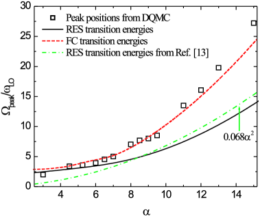
Figure 2: The transition energy for the transition from the polaron ground state to the first RES(solid black curve) and to the first excited FC state (dashed red curve) as a function of $\alpha$ obtained in the present work, compared with the maximum of the polaron optical conductivity band from numerical DQMC (black squares, Ref. [12]). The dashed-dot green curve: the strong-coupling result for this transition energy as given in Ref. [14].

For $\alpha\lesssim 2.5$, there exists no minimum of $E_{p}^{\left(1exc\right)}$ in the range $v>1$. We can interpret this result as a manifestation of the fact that for decreasing coupling strength, the RES is suppressed at sufficiently weak coupling. We see that for sufficiently small $\alpha$ ($\alpha\lesssim 6$), the RES transition energies show good agreement with the DQMC peak energies, what confirms the concept of RES developed in Refs. [7, 14]. For higher coupling strengths, the DQMC data appear to be closer to the FC (rather than to RES) transition energies. This result can be an indication of the fact that with increasing $\alpha$, the mechanism of the polaron optical absorption changes its nature as suggested in Ref. [13], from a regime with dynamic lattice relaxation (for which the RES are relevant) at weak and intermediate coupling to the Franck-Condon (“LO-phonon sidebands”-) regime at strong coupling.

In summary, we have re-formulated the Feynman all-coupling path integral method for the polaron problem within a Hamiltonian formalism using time-ordered operator calculus. This reformulation allows us to describe not only the free energy and the ground state, but also to directly determine – for the first time – the excited polaron states that correspond to the Feynman all-coupling polaron model. A variational procedure for the polaron RES energy has been developed, within the formalism presented in this work, which provides results i.a. in agreement with the strong-coupling limit of Ref. [14]. The present treatment offers the prospect of further elucidation of the nature of the polaron resonances (“relaxed excited states” versus “Franck-Condon sidebands” [9]) at intermediate coupling.

This work was supported by FWO-V projects G.0356.06, G.0370.09N, G.0180.09N, G.0365.08, and the WOG WO.035.04N (Belgium).

References

- [1] This work was presented at the 10th International Conference “Path Integrals – 2010”, July 11 – 16, 2010, Washington DC, USA.
- [2] N. N. Bogolubov and N. N. Bogolubov, Jr., Some Aspects of Polaron Theory. In: Lecture Notes in Physics vol. 4, World Scientific, Singapore (1988).
- [3] R. P. Feynman, Phys. Rev. 97, 660 (1955).
- [4] K. Yamazaki, J. Phys. A 16, 3675 (1983).
- [5] V. Cataudella, G. De Filippis, and C. A. Perroni, in Polarons in Advanced Materials, Springer Series in Materials Science , Vol. 103, Edited by A. S. Alexandrov (Canopus and Springer, Bath, UK, 2007), pp. 149 – 189.
- [6] R. P. Feynman, R. W. Hellwarth, C. K. Iddings, and P. M. Platzman, Phys. Rev. 127, 1004 (1962).
- [7] J. Devreese, J. De Sitter, and M. Goovaerts, Phys. Rev. B 5, 2367 (1972).
- [8] F. M. Peeters and J. T. Devreese, Phys. Rev. B 28, 6051 (1983).
- [9] R. Evrard, Phys. Lett. 14, 295 (1965); J. T. Devreese and A. S. Alexandrov, Rep. Prog. Phys. 72, 066501 (2009).
- [10] J. T. Devreese and R. Evrard , Phys. Lett. 11, 278 (1964).
- [11] J. T. Devreese and F. Brosens, Phys. Rev. B 45, 6459 (1992).
- [12] A. S. Mishchenko, N. Nagaosa, N. V. Prokof’ev, A. Sakamoto, and B. V. Svistunov, Phys. Rev. Lett. 91, 236401 (2003).
- [13] G. De Filippis, V. Cataudella, A. S. Mishchenko, C. A. Perroni, and J. T. Devreese, Phys. Rev. Lett. 96, 136405 (2006).
- [14] E. Kartheuser, R. Evrard, and J. Devreese, Phys. Rev. Lett. 22, 94 (1969).
- [15] Y. Lépine and M. Charbonneau, Phys. Status Solidi B 122, 151 (1984); Y. Frongillo and Y. Lépine, Phys. Rev. B 40, 3570 (1989).