Analysis of the sensitivity to discrete dividends :
A new approach for pricing vanillas

Abstract

The incorporation of a dividend yield in the classical option pricing model of Black-Scholes results in a minor modification of the Black-Scholes formula, since the lognormal dynamic of the underlying asset is preserved. However, market makers prefer to work with cash dividends with fixed value instead of a dividend yield. Since there is no closed-form solution for the price of a European Call in this case, many methods have been proposed in the literature to approximate it. Here, we present a new approach. We derive an exact analytic formula for the sensitivity to dividends of an European option. We use this result to elaborate a proxy which possesses the same Taylor expansion around 0 with respect to the dividends as the exact price. The obtained approximation is very fast to compute (the same complexity than the usual Black-Scholes formula) and numerical tests show the extreme accuracy of the method for all practical cases.


Key words: Equity options, discrete dividends.

1 Introduction

In the classical Black-Scholes framework, we can find in the literature three main ways of inserting cash dividends into the model :

1. Escrowed model. Assume that the asset price minus the present value of all dividends to be paid before the maturity of the option follows a Geometric Brownian Motion.

2. Forward model. Assume that the asset price plus the forward value of all dividends from past dividend dates to today, follows a Geometric Brownian Motion.

3. Piecewise lognormal model. Assume that the asset price shows a jump downward at each dividend date (equal to the cash dividend payment at that date) and follows a Geometric Brownian Motion between those dates.

Although the first two models lead to a closed-form solution, they are not satisfactory. Indeed, the option price obtained in these models is not continuous at dividend dates. Moreover, if one considers two options with different maturities $T_{1}<T_{2}$, the first two models lead to different asset price process dynamics for $t\leq T_{1}$, since the dividends paid between $T_{1}$ and $T_{2}$ are taken into account in one case but not in the other.

Therefore, it is the piecewise lognormal model which is prefered from a theoritical point of view. This paper is dedicated to find a robust pricing proxy for this model. We consider an underlying following a Black-Scholes dynamic between dividend detachement dates and paying cash dividends at discrete times $0<T_{1}<\ldots<T_{n}<T$, i.e. :

• for $T_{i}\leq t<T_{i+1}$ :

  $$dS_{t}=rS_{t}dt+\sigma S_{t}dW_{t},$$

• at time $T_{i}$ :

  $$S_{T_{i}^{+}}=S_{T_{i}^{-}}-D_{i}(S_{T_{i}^{-}}),$$

where $r$ is the interest rate, assumed constant, $W$ is a standard Brownian motion and $D_{i}$ is the dividend policy defined by :

$$D_{i}(S)=\left\{\begin{array}[]{lll}C_{i}&\text{if}&S>C_{i},\\ S&\text{if}&S\leq C_{i},\end{array}\right.$$

The cash amounts $C_{1},\ldots,C_{n}$ are known at the initial date 0 and each $C_{i}$ represents the dividend cash amount eventually paid at time $T_{i}$.

The dividend policy $D_{i}$ is a liquidator policy as the stock price is absorbed at zero at time $T_{i}$ if $S_{T_{i}}<C_{i}$. Consequently, the stock price remains positive. Note that as a practical matter, for most applications, the definition of $D_{i}(S)$ when $S\leq C_{i}$ has negligible financial effects, as the probability that a stock price drops below a declared dividend at a fixed time is typically small. It just ensures the positivity of the price.

In this paper, we are interested in computing the fair price of the European Call $\operatorname*{Call}(S_{0},K)$ with strike $K$ and maturity $T$. Since there is no closed-formula, one should recover the price via PDE methods using a finite difference scheme, with boundary conditions at each $T_{i}$ ensuring the continuity of the price of the Call. This procedure can be time-consuming if one considers a maturity $T=20$ years and an underlying paying as much as one dividend a week. Therefore, when computation speed is at stake, one would prefer a fast and accurate proxy for the price.

We review in the following section three of the existing methods in the literature and discuss their limitations.

2 Existing Methods

1. Method of moments matching. We approximate the stock price process $S$ by a process $\tilde{S}$ with a shifted log-normal dynamic under the risk-neutral pricing measure :

   $$\tilde{S}_{t}=\lambda+M\exp\left(-\frac{1}{2}\sigma^{{}^{\prime}2}t+\sigma^{{}^{\prime}}W_{t}\right).$$

   The three parameters $\lambda,M$ and $\sigma^{{}^{\prime}}$ are calibrated so that the first three moments of $\tilde{S}_{T}$ match the first three moments of $S_{T}$. This method reduces to the pricing of a European Call on a modified underlying $\tilde{S}$, which can be done using the usual Black-Scholes formula. This proxy does not work well if the stock pays dividends frequently, the maturity is greater than 5 years or the option is deep in-the-money.

2. In [1], Bos and Vandermark define a mixture of the Escrowed and Forward models, using linear pertubations of first order. They derive a proxy resulting in spot/strike adjustment :

   $$\operatorname*{Call}(S_{0},K)\approx\operatorname*{Call^{BS}}(S^{\ast},K^{\ast}),$$

   where $\operatorname*{Call^{BS}}$ is the usual Black-Scholes function and:

   $$S^{\ast}= S_{0}-\sum_{i=1}^{n}\left(1-\frac{T_{i}}{T}\right)C_{i}e^{-rT_{i}},$$ (1)

   $$K^{\ast}= K+\sum_{i=1}^{n}\frac{T_{i}}{T}C_{i}e^{r(T-T_{i})}.$$ (2)

   This proxy works better for at-the-money options and small maturities but results in serious mis-pricing for in-and out-of-the-money options and large maturities.

3. In [2], Bos, Gairat and Shepeleva derive a more accurate proxy than the previous one by considering a volatility adjustment :

   $$\operatorname*{Call}(S_{0},K)\approx\operatorname*{Call^{BS}}(S^{\ast},K,\sigma(S^{\ast},K,T)),$$

   with $S^{\ast}$ given by (1):

   $$\sigma(S^{\ast},K,T)^{2}= \sigma^{2}+\sigma\sqrt{\frac{\pi}{2T}}\Bigg{\{}\frac{e^{\frac{a^{2}}{2}}}{S^{\ast}}\sum_{i=1}^{n}C_{i}e^{-rT_{i}}\left[N(a)-N\left(a-\sigma\frac{T_{i}}{\sqrt{T}}\right)\right]$$

   $$+ \frac{e^{\frac{b^{2}}{2}}}{S^{\ast 2}}\sum_{i,j=1}^{n}C_{i}C_{j}e^{-r(T_{i}+T_{j})}\left[N(b)-N\left(b-2\sigma\frac{min(T_{i},T_{j})}{\sqrt{T}}\right)\right],$$

   where $N(x)$ is the normal distribution function and:

   $$a=\frac{1}{\sigma\sqrt{T}}\left(\log\left(\frac{S^{\ast}}{K}\right)+(r-\sigma^{2}/2)T\right),\ b=a+\frac{1}{2}\sigma\sqrt{T}.$$

   This proxy will be a good benchmark to test the accuracy of our method presented in the following section.

3 The method

3.1 Motivations and notations

Consider $\operatorname*{Call}(S_{0},K)$ as a function of the dividends $C_{1},\ldots,C_{n}$:

$$\operatorname*{Call}(S_{0},K)=\operatorname*{Call}(C_{1},\ldots,C_{n}).$$

Although there is no closed-form formula for $\operatorname*{Call}(C_{1},\ldots,C_{n})$, we prove in annex A that we can still compute explicitely its sensitivities to dividends at the origin. More precisely, we have for all $k\in\mathbb{N}$ and $1\leq i_{1},\ldots,i_{k}\leq n$:

$$\frac{\partial^{k}\operatorname*{Call}}{\partial C_{i_{1}}\ldots\partial C_{i_{k}}}(0)=(-1)^{k}\frac{\partial^{k}\operatorname*{Call^{BS}}}{\partial S^{k}}\left(S_{0}e^{-\sigma^{2}\sum_{q=1}^{k}T_{i_{q}}},K,T\right)e^{-r\sum_{q=1}^{k}T_{i_{q}}-\sigma^{2}\sum_{q=2}^{k}(q-1)T_{i_{q}}}.$$ (3)

We use this result to derive an accurate approximation of $\operatorname*{Call}(C_{1},\ldots,C_{n})$. Before explaining our method, we need first to introduce some notations. For all functions $f$ of $n$ variables $x_{1},\ldots,x_{n}$ and $\forall\alpha\in\mathbb{N}$, we note $T_{\alpha}f$ the $\alpha^{th}$ order Taylor series at 0 of $f$:

$$T_{\alpha}f(x_{1},\ldots,x_{n}):=\sum_{k=0}^{\alpha}\sum_{i_{1},\ldots,i_{k}=1}^{n}\frac{x_{i_{1}}\ldots x_{i_{k}}}{i_{1}!\ldots i_{k}!}\frac{\partial^{k}f}{\partial x_{i_{1}}\ldots\partial x_{i_{k}}}(0).$$

We introduce the space $\mathcal{A}_{\alpha}$ of functions having the same $\alpha^{th}$ Taylor series at 0 as the function $\operatorname*{Call}(C_{1},\ldots,C_{n})$:

$$\mathcal{A}_{\alpha}:=\{f,T_{\alpha}f=T_{\alpha}\operatorname*{Call}\}.$$

The order $\alpha$ quantifies how near is $f(C_{1},\ldots,C_{n})$ from $\operatorname*{Call}(C_{1},\ldots,C_{n})$ when the dividends are small. This precision increase with $\alpha$.

Functions $f$ in $\mathcal{A}_{\alpha}$ are naturally good candidates to approximate $\operatorname*{Call}$. However, the difference $\operatorname*{Call}(C_{1},\ldots,C_{n})-f(C_{1},\ldots,C_{n})$ can be quite big if the dividends are not small enough. For instance, for $\alpha=2$ and 3, we test the accuracy of the natural choice consisting of taking

$$f(C_{1},\ldots,C_{n}):=T_{\alpha}\operatorname*{Call}(C_{1},\ldots,C_{n}).$$

Figure 1 shows the relative error of the price of a European Call when using this approximation. We assume that the stock pays a fixed dividend $C$ every year and we analyse how the relative error varies when we increase $C$. We can see that both the second and third order Taylor series give accurate results when the dividends are small but when the dividends increase, they both lead to serious mis-pricing.

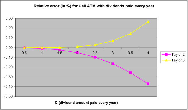
Figure 1: Relative Error using the Taylor series for approximation. Numerical parameters: $S_{0}=100,K=100,r=3\%,\sigma=30\%,T=10y$.

Therefore, the approximations $T_{\alpha}\operatorname*{Call}$, $\alpha=2,3$, are not satisfying. Thus, one need to find for $\alpha\geq 2$, a function $\operatorname*{Proxy}\in\mathcal{A}_{\alpha}$, different from $T_{\alpha}\operatorname*{Call}$, which gives an accurate approximation of $\operatorname*{Call}$ for all practical values of $C_{1},\ldots,C_{n}$ (not necessarily very small). We explain in the next subsection how we determine $\operatorname*{Proxy}\in\mathcal{A}_{\alpha}$.

3.2 Spot/Strike adjustment

Like Bos and Vandermark in [1], we search our function $\operatorname*{Proxy}$ under the form:

$$\operatorname*{Proxy}(C_{1},\ldots,C_{n}):=\operatorname*{Call^{BS}}(S^{\ast}(C_{1},\ldots,C_{n}),K^{\ast}(C_{1},\ldots,C_{n})),$$ (4)

with:

$$S^{*}(C_{1},\ldots,C_{n})= S_{0}+\sum_{k=0}^{\alpha}\sum_{i_{1},\ldots,i_{k}=1}^{n}a_{i_{1},\ldots,i_{k}}C_{i_{1}}\ldots C_{i_{k}},$$ (5)

$$K^{*}(C_{1},\ldots,C_{n})= K+\sum_{k=0}^{\alpha}\sum_{i_{1},\ldots,i_{k}=1}^{n}b_{i_{1},\ldots,i_{k}}C_{i_{1}}\ldots C_{i_{k}}.$$ (6)

The reason why we perform a spot/strike adjustment is that it allows to recover the exact price when the dividends are paid spot or at maturity.

The coefficients $a_{i_{1},\ldots,i_{k}}$ and $b_{i_{1},\ldots,i_{k}}$ are calculated recursively. They are entirely determined by the two following conditions:

1. $\frac{\partial^{k}\operatorname*{Proxy}}{\partial C_{i_{1}}\ldots\partial C_{i_{k}}}(0)=\frac{\partial^{k}\operatorname*{Call}}{\partial C_{i_{1}}\ldots\partial C_{i_{k}}}(0),\forall k\leq\alpha$,

2. We impose our proxy to satisfy the Call-Put parity:

   $$\operatorname*{Call^{BS}}(S^{\ast},K^{\ast})-\operatorname*{Put^{BS}}(S^{*},K^{*})= S_{0}-Ke^{-rT}-\sum_{i=1}^{n}C_{i}e^{-rT_{i}},$$ (7)

   $$i.e.\hskip 99.58464ptS^{\ast}-K^{\ast}e^{-rT}= S_{0}-Ke^{-rT}-\sum_{i=1}^{n}C_{i}e^{-rT_{i}}.$$ (8)

Let’s detail the calculus:

• Computation of $a_{i}$ and $b_{i}$: the equality $\frac{\partial\operatorname*{Proxy}}{\partial C_{i}}(0)=\frac{\partial\operatorname*{Call}}{\partial C_{i}}(0)$ reads:

  $$N(d_{1})a_{i}-e^{-rT}N(d_{2})b_{i}=-e^{-rT_{i}}N(d(T_{i})),$$ (9)

  where :

  $$d_{1}= \frac{1}{\sigma\sqrt{T}}(\ln(S_{0}/K)+(r+\sigma^{2}/2)T),$$

  $$d_{2}= d_{1}-\sigma\sqrt{T},$$

  $$d(t)= d_{1}-\frac{\sigma}{\sqrt{T}}t,\hskip 14.22636pt0\leq t\leq T.$$

  The differentiation of (8) writes:

  $$a_{i}-e^{-rT}b_{i}=-e^{-rT_{i}}.$$ (10)

  Solving the linear system (9)-(10) gives:

  $$a_{i}= -e^{-rT_{i}}\frac{N(d(T_{i}))-N(d_{2})}{N(d_{1})-N(d_{2})},$$

  $$b_{i}= e^{r(T-T_{i})}\frac{N(d_{1})-N(d(T_{i}))}{N(d_{1})-N(d_{2})}.$$

• Computation of $a_{i,j}$ and $b_{i,j}$: the equality $\frac{\partial^{2}\operatorname*{Proxy}}{\partial C_{i}\partial C_{j}}(0)=\frac{\partial^{2}\operatorname*{Call}}{\partial C_{i}\partial C_{j}}(0)$ and two succesive differentiations in (8) give the following linear system:

  $$N(d_{1})a_{i,j}-e^{-rT}N(d_{2})b_{i,j}= \beta,$$ (11)

  $$a_{i,j}-e^{-rT}b_{i,j}= 0,$$ (12)

  where:

  $$\beta=\frac{\partial^{2}\operatorname*{Call}}{\partial C_{i}\partial C_{j}}(0)-a_{i}a_{j}\frac{\partial^{2}\operatorname*{Call^{BS}}}{\partial S^{2}}(S_{0},K)-(a_{i}b_{j}+a_{j}b_{i})\frac{\partial^{2}\operatorname*{Call^{BS}}}{\partial S\partial K}(S_{0},K)-b_{i}b_{j}\frac{\partial^{2}\operatorname*{Call^{BS}}}{\partial K^{2}}(S_{0},K).$$

  After some direct computations, we obtain:

  $$a_{i,j}= \frac{1}{\gamma}e^{-r(T_{i}+T_{j})}\Bigg{[}a+b\Big{(}N(d(T_{i}))+N(d(T_{j}))\Big{)}+cN(d(T_{i}))N(d(T_{j}))+de^{\sigma^{2}T_{i}}N^{{}^{\prime}}(d(T_{i}+T_{j}))\Bigg{]},$$

  $$b_{i,j}= e^{rT}a_{i,j},$$

  with:

  $$\gamma= \sigma S\sqrt{T}N^{{}^{\prime}}(d_{1})\Big{(}N(d_{1})-N(d_{2})\Big{)}^{3}$$

  $$a= -\Big{(}N(d_{2})N^{{}^{\prime}}(d_{1})-N(d_{1})N^{{}^{\prime}}(d_{2})\Big{)}^{2}$$

  $$b= \Big{(}N^{{}^{\prime}}(d_{1})-N^{{}^{\prime}}(d_{2})\Big{)}\Big{(}N(d_{2})N^{{}^{\prime}}(d_{1})-N(d_{1})N^{{}^{\prime}}(d_{2})\Big{)}$$

  $$c= -\Big{(}N^{{}^{\prime}}(d_{1})-N^{{}^{\prime}}(d_{2})\Big{)}^{2}$$

  $$d= N^{{}^{\prime}}(d_{1})\Big{(}N(d_{1})-N(d_{2})\Big{)}^{2}$$

• Computation of $a_{i_{1},\ldots,i_{k}}$ and $b_{i_{1},\ldots,i_{k}}$, $k\geq 3$: the previous method can be reproduced recursively. Knowing all the values $a_{j_{1},\ldots,j_{m}}$ and $b_{j_{1},\ldots,j_{m}}$, $m\leq k-1$, we obtain $a_{i_{1},\ldots,i_{k}}$ and $b_{i_{1},\ldots,i_{k}}$ by solving a linear system of the form :

  $$\frac{\partial^{k}\operatorname*{Call^{BS}}}{\partial S^{k}}(S_{0},K)a_{i_{1},\ldots,i_{k}}+\frac{\partial^{k}\operatorname*{Call^{BS}}}{\partial K^{k}}(S_{0},K)b_{i_{1},\ldots,i_{k}}= u,$$

  $$a_{i_{1},\ldots,i_{k}}-e^{-rT}b_{i_{1},\ldots,i_{k}}= 0.$$

We have presented a simple and general method to derive a function $\operatorname*{Proxy}$ in $\mathcal{A}_{\alpha}$ for any $\alpha\in\mathbb{N}$. As for the order $\alpha$ that we choose effectively for our tests, the second order computation is a good choice for performance and accuracy. Before presenting the numerical results, we recall some desirable properties of our second order proxy (4):

1. fast computation, even when one considers a large number $n$ of dividends.

2. recovery of exact price when all dividends are paid spot or at maturity.

3. arbitrage free with the Call-Put parity.

4. guarantee of the continuity of the Call price at dividend detachement dates.

5. accuracy for all practical configurations, even for the extreme cases (deep in-the-money-option with large maturity and high frequency of dividends) for which the already existing methods of the financial literature might lead to serious mis-pricing.

4 Numerical tests

4.1 Test on an underlying paying dividends with low frequency

We test the accuracy of our proxy on a stock with the following parameters: $S_{0}=100$, $r=3\%$, $\sigma=30\%$. We suppose that the stock pays a dividend of 3 in the middle of every year. We compute the Call price with strike $K\in\{50,75,100,125,150,175,200\}$ and maturity $T\in\{5,10,15,20\}$ using four methods:

1. the finite difference method,

2. the method of moments matching.

3. the spot/vol adjustment of Bos, Gairat and Shepeleva[2],

4. our proxy with spot/strike adjustment given by (5)-(6),

Remember that no approximation is made in the finite difference method. The results are given in the following tables.

Maturity=5 years
$K/S_{0}$	0.5	0.75	1	1.25	1.50	1.75	2
Price:
FD (exact price)	47.14	33.85	24.42	17.79	13.12	9.79	7.39
Method of moments	47.17	33.87	24.42	17.78	13.10	9.77	7.38
Proxy BGS	47.11	33.84	24.42	17.80	13.13	9.81	7.41
Proxy GS	47.14	33.85	24.42	17.79	13.12	9.79	7.39
Relative error (in%):
Method of moments	0.07	0.06	0.01	-0.05	-0.11	-0.16	-0.20
Proxy BGS	-0.05	-0.05	-0.02	0.03	0.10	0.17	0.24
Proxy GS	0.00	0.00	0.00	0.00	0.00	0.00	0.00

Maturity=10 years
$K/S_{0}$	0.5	0.75	1	1.25	1.50	1.75	2
Price:
FD (exact price)	46.85	38.21	31.66	26.58	22.56	19.34	16.71
Method of moments	47.07	38.38	31.77	26.64	22.59	19.34	16.69
Proxy BGS	46.65	38.08	31.59	26.57	22.60	19.41	16.81
Proxy GS	46.85	38.21	31.66	26.58	22.56	19.34	16.71
Relative error (in%):
Method of moments	0.49	0.45	0.35	0.23	0.11	-0.01	-0.13
Proxy BGS	-0.43	-0.35	-0.21	-0.04	0.15	0.35	0.55
Proxy GS	0.00	-0.01	-0.01	-0.01	-0.01	-0.01	-0.02

Maturity=15 years
$K/S_{0}$	0.5	0.75	1	1.25	1.50	1.75	2
Price:
FD (exact price)	46.47	40.48	35.73	31.85	28.63	25.91	23.59
Method of moments	47.12	41.04	36.18	32.21	28.91	26.13	23.75
Proxy BGS	45.79	40.01	35.43	31.70	28.60	25.98	23.74
Proxy GS	46.49	40.49	35.73	31.85	28.63	25.91	23.59
Relative error (in%):
Method of moments	1.41	1.38	1.27	1.13	0.98	0.82	0.66
Proxy BGS	-1.47	-1.19	-0.85	-0.49	-0.12	0.24	0.60
Proxy GS	0.02	-0.01	-0.02	-0.03	-0.03	-0.04	-0.04

Maturity=20 years
$K/S_{0}$	0.5	0.75	1	1.25	1.50	1.75	2
Price:
FD (exact price)	46.02	41.74	38.22	35.26	32.72	30.51	28.57
Method of moments	47.35	42.95	39.30	36.21	33.55	31.24	29.20
Proxy BGS	44.33	40.47	37.30	34.63	32.33	30.32	28.55
Proxy GS	46.10	41.76	38.23	35.26	32.71	30.50	28.56
Relative error (in%):
Method of moments	2.89	2.90	2.82	2.69	2.54	2.38	2.21
Proxy BGS	-3.71	-3.07	-2.44	-1.82	-1.23	-0.65	-0.09
Proxy GS	0.14	0.03	-0.02	-0.04	-0.05	-0.06	-0.07

4.2 Test on an underlying paying dividends with high frequency

We now check the accuracy of our proxy on an underlying paying dividends every week. This situation occurs when considering an index like S&P 500 or Eurostox 50. We take the following parameters: $S_{0}=3000$, $r=3\%$, $\sigma=30\%$. We suppose that the stock pays a dividend of 2 every week. We compute the Call price with strike $K$ such as $K/S_{0}\in\{0.5,0.75,1,1.25,1.5,1.75,2\}$ and maturity $T\in\{5,10,15,20\}$.

Maturity=5 years
$K/S_{0}$	0.5	0.75	1	1.25	1.50	1.75	2
Price:
FD (exact price)	1359.87	972.67	699.65	508.71	374.45	279.07	210.47
Method of moments	1361.05	973.29	699.70	508.39	373.97	278.54	209.98
Proxy BGS	1358.88	972.02	699.52	508.99	375.00	279.75	211.21
Proxy GS	1359.87	972.69	699.68	508.73	374.47	279.07	210.47
Relative error (in%):
Method of moments	0.09	0.06	0.01	-0.06	-0.13	-0.19	-0.23
Proxy BGS	-0.07	-0.07	-0.02	0.05	0.15	0.25	0.35
Proxy GS	0.00	0.00	0.00	0.00	0.00	0.00	0.00

Maturity=10 years
$K/S_{0}$	0.5	0.75	1	1.25	1.50	1.75	2
Price:
FD (exact price)	1319.62	1075.07	890.03	746.82	633.81	543.14	469.40
Method of moments	1327.05	1080.52	893.49	748.67	634.44	542.91	468.55
Proxy BGS	1311.37	1069.84	887.68	746.80	635.57	546.23	473.42
Proxy GS	1319.68	1075.04	889.96	746.72	633.69	543.02	469.25
Relative error (in%):
Method of moments	0.56	0.51	0.39	0.25	0.10	-0.04	-0.18
Proxy BGS	-0.63	-0.49	-0.26	0.00	0.28	0.57	0.86
Proxy GS	0.00	0.00	-0.01	-0.01	-0.02	-0.02	-0.03

Maturity=15 years
$K/S_{0}$	0.5	0.75	1	1.25	1.50	1.75	2
Price:
FD (exact price)	1287.50	1122.13	990.74	883.63	794.68	719.49	655.20
Method of moments	1308.65	1140.08	1005.32	895.16	803.52	726.17	660.09
Proxy BGS	1258.42	1102.31	978.74	877.99	794.07	723.01	662.03
Proxy GS	1288.47	1122.33	990.66	883.42	794.31	719.10	654.79
Relative error (in%):
Method of moments	1.64	1.60	1.47	1.31	1.11	0.93	0.75
Proxy BGS	-2.26	-1.77	-1.21	-0.64	-0.08	0.49	1.04
Proxy GS	0.08	0.02	-0.01	-0.02	-0.05	-0.06	-0.06

Maturity=20 years
$K/S_{0}$	0.5	0.75	1	1.25	1.50	1.75	2
Price:
FD (exact price)	1260.33	1144.53	1049.11	968.59	899.43	839.22	786.23
Method of moments	1303.36	1183.64	1083.92	999.27	926.36	862.79	806.82
Proxy BGS	1184.43	1088.21	1008.55	940.91	882.41	831.09	785.57
Proxy GS	1264.53	1145.94	1049.44	968.43	899.04	838.71	785.66
Relative error (in%):
Method of moments	3.41	3.42	3.32	3.17	2.99	2.81	2.62
Proxy BGS	-6.02	-4.92	-3.87	-2.86	-1.89	-0.97	-0.08
Proxy GS	0.33	0.12	0.03	-0.02	-0.04	-0.06	-0.07

5 Conclusion

We have presented a new approach to deal with cash dividends in equity option pricing in a piecewise lognormal model for the underlying. Our method relies on the derivation of an analytic formula for the sensitivity to dividends of a European option. We obtain a closed-form formula for a European Call which gives both very accurate results for all practical cases.

Appendix A Computation of the dividend sensitivities

Consider a European option of maturity $T$ with payoff $h(S_{T})$, with $S$ the stock price following the piecewise lognormal dynamic presented in the introduction. We note its fair price at time 0

$$\Pi(S_{0},T,C_{1},\ldots,C_{n})$$

We denote:

$$\Pi^{BS}(S_{0},T)$$

the fair price of the option if $S$ does not pay dividends. The partial derivatives

$$\frac{\partial^{k}\Pi}{\partial C_{i_{1}}\ldots\partial C_{i_{k}}}(S_{0},T,0,\ldots,0)$$

are related to the usual Black-Scholes greeks by the following formula:

Proposition A.1

For $k\in\mathbb{N}$ and $1\leq i_{1}\leq\ldots\leq i_{k}\leq n$, we have:

$$\frac{\partial^{k}\Pi}{\partial C_{i_{1}}\ldots\partial C_{i_{k}}}(S_{0},T,0,\ldots,0)=(-1)^{k}\frac{\partial^{k}\Pi^{BS}}{\partial S^{k}}\left(S_{0}e^{-\sigma^{2}\sum_{q=1}^{k}T_{i_{q}}},T\right)e^{-r\sum_{q=1}^{k}T_{i_{q}}-\sigma^{2}\sum_{q=2}^{k}(q-1)T_{i_{q}}}.$$

Follows a proof of this formula.

A.1 First step: a recursive formula

We introduce some notations:

• We define the natural filtration $(\mathcal{F}_{t})_{t\geq 0}$ associated with the brownian motion $W$. We suppose the filtration right continuous.

• We define for all $0\leq t_{1}\leq t_{2}$:

  $$X_{t_{1}\to t_{2}}:=e^{(r-\sigma^{2}/2)(t_{2}-t_{1})+\sigma(W_{t_{2}}-W_{t_{1}})},$$

• We denote $\phi(S_{0},S,t)$ the log-normal density associated with the variable $S_{0}X_{0\rightarrow t}$

• We define the functions of $n+1$ variables $(h_{i})_{0\leq i\leq n}$ such as:

  $$h_{i}(S_{T_{i}},C_{1},\ldots,C_{n}):=e^{-r(T-T_{i})}E[h(S_{T})|\mathcal{F}_{T_{i}}].$$

For the sake of simplicity, when there is no confusion, we will simply denote $h_{i}(S)$ instead of $h_{i}(S,C_{1},\ldots,C_{n})$. Note that we have $\Pi(S_{0},T,C_{1},\ldots,C_{n})=h_{0}(S_{0})$. We can compute the functions $h_{i}$ recursively beginning with $h_{n}$:

$$h_{n}(S)=\Pi^{BS}(S,T-T_{n}),$$

and by conditioning, $\forall i\leq n-1$:

$$h_{i}(S)= e^{-r(T_{i+1}-T_{i})}E[h_{i+1}((SX_{t_{i}\rightarrow t_{i+1}}-C_{i+1})_{+})|\mathcal{F}_{T_{i}}]$$

$$= e^{-r(T_{i+1}-T_{i})}\int_{C_{i+1}}^{\infty}h_{i+1}(S_{i+1}-C_{i+1})\phi(S,S_{i+1},T_{i+1}-T_{i})dS_{i+1},$$ (13)

Now, we show how these relations allow us to compute recursively the partial derivatives:

$$\frac{\partial^{k}\Pi}{\partial C_{i_{1}}\ldots\partial C_{i_{k}}}(S_{0},0,\ldots,0),$$

for $1\leq i\leq n$, $k\in\mathbb{N}^{\ast}$ and $1\leq i_{1}\leq\ldots\leq i_{k}\leq n$. First, note that a direct application of the theorem of differentiation under the integral sign in the relation (13) proves that the functions $h_{i}$, $0\leq i\leq n$ are infinitely differentiable. Then, using the markov property of the log-normal densities:

$$\int_{0}^{\infty}\phi(S_{i},S_{i+1},t_{i})\phi(S_{i+1},S_{i+2},t_{i+1})dS_{i+1}=\phi(S_{i},S_{i+2},t_{i}+t_{i+1}),$$

we obtain:

$$\frac{\partial^{k}\Pi}{\partial C_{i_{1}}\ldots\partial C_{i_{k}}}(S_{0},0,\ldots,0)= -e^{-rT_{i_{1}}}E\left[\frac{\partial^{k}h_{i_{1}}}{\partial S\partial C_{i_{2}}\ldots\partial C_{i_{k}}}(S_{0}X_{0\rightarrow T_{i_{1}}},0,\ldots,0)\right],$$

$$= -e^{-rT_{i_{1}}}\int_{0}^{\infty}\frac{\partial^{k}h_{i_{1}}}{\partial S\partial C_{i_{2}}\ldots\partial C_{i_{k}}}(S_{i_{1}},0,\ldots,0)\phi(S_{0},S_{i_{1}},T_{i_{1}})dS_{i_{1}}.$$ (14)

This relation will be very useful for a recursive proof of proposition A.1 since it reduces by one the number of differentiations with respect to the dividends.

A.2 Second step: a martingale argument

The proof of proposition A.1 relies heavily on this simple but crucial lemma:

Lemma A.2

Consider a process following a Black-Scholes dynamic $S_{t}=S_{0}e^{(r-\sigma^{2}/2)t+\sigma W_{t}}$, $0\leq t\leq T$. Then, for all integer $k\geq 0$ and for all real number $a\geq 0$, the process:

$$Z_{t}:=\frac{\partial^{k}\Pi^{BS}}{\partial S^{k}}\left(S_{t}e^{k\sigma^{2}(t-a)},T-t\right)e^{(k-1)(r+k\sigma^{2}/2)t}$$

is a martingale.

The following corollary is easy to derive.

Corollary A.3

For $k\in\mathbb{N}^{*}$, $0\leq t\leq T$ and $a\geq 0$, we have:

$$E\left[\frac{\partial^{k}\Pi^{BS}}{\partial S^{k}}\left(S_{t}e^{k\sigma^{2}(t-a)},T-t\right)\right]=\frac{\partial^{k}\Pi^{BS}}{\partial S^{k}}\left(S_{0}e^{-k\sigma^{2}a},T\right)e^{-(k-1)(r+k\sigma^{2}/2)t}$$ (15)

Proof of lemma A.2: The drift of $Z_{t}$ is:

$$e^{(k-1)(r+k\sigma^{2}/2)t}\Bigg{[}(k-1)(r+k\sigma^{2}/2)\frac{\partial^{k}\Pi^{BS}}{\partial S^{k}}-\frac{\partial^{k+1}\Pi^{BS}}{\partial t\partial S^{k}}$$

$$+(r+k\sigma^{2})S_{t}e^{k\sigma^{2}(t-a)}\frac{\partial^{k+1}\Pi^{BS}}{\partial S^{k+1}}+\frac{1}{2}\sigma^{2}S_{t}^{2}e^{2k\sigma^{2}(t-a)}\frac{\partial^{k+2}\Pi^{BS}}{\partial S^{k+2}}\Bigg{]},$$ (16)

where all the derivatives in the last formula are evaluated in $(S_{t}e^{k\sigma^{2}(t-a)},T-t)$. Remember that $\Pi^{BS}$ satisfies the Black-Scholes PDE:

$$-\frac{\partial\Pi^{BS}}{\partial t}+\frac{1}{2}\sigma^{2}S^{2}\frac{\partial^{2}\Pi^{BS}}{\partial S^{2}}+rS\frac{\partial\Pi^{BS}}{\partial S}-r\Pi^{BS}=0.$$

Now, differentiate $k$ times this equation with respect to $S$:

$$-\frac{\partial^{k+1}\Pi^{BS}}{\partial t\partial S^{k}}+\frac{1}{2}\sigma^{2}S^{2}\frac{\partial^{k+2}\Pi^{BS}}{\partial S^{k+2}}+(r+k\sigma^{2})S\frac{\partial^{k+1}\Pi^{BS}}{\partial S^{k+1}}+(k-1)(r+k\sigma^{2}/2)\frac{\partial^{k}\Pi^{BS}}{\partial S^{k}}=0.$$ (17)

One immediately checks that the term in bracket in (16) is equal to the left term in (17) evaluated in $(S_{t}e^{k\sigma^{2}(t-a)},T-t)$, and therefore is equal to 0.

$\Box$

A.3 Third step: Proof of proposition A.1

We argue by recurrence on the number $k$ of differentiations with respect to the dividends:

• If $k=0$, the proposition is trivially true as it simply says:

  $$\Pi(S_{0},T,0,\ldots,0)=\Pi^{BS}(S,T).$$

• Now, suppose that the property is true at rank $k$. We want to prove that it remains true at rank $k+1$. We have by relation (14):

  $$\frac{\partial^{k+1}\Pi}{\partial C_{i_{1}}\ldots\partial C_{i_{k+1}}}(S_{0},0,\ldots,0)= -e^{-rT_{i_{1}}}E\left[\frac{\partial^{k+1}h_{i_{1}}}{\partial S\partial C_{i_{2}}\ldots\partial C_{i_{k+1}}}(S_{0}X_{0\to T_{i_{1}}},0,\ldots,0)\right].$$ (18)

  By hypothesis of recurrence, we have:

  $$\frac{\partial^{k}h_{i_{1}}}{\partial C_{i_{2}}\ldots\partial C_{i_{k+1}}}(S,0,\ldots,0)$$

  $$=(-1)^{k}\frac{\partial^{k}\Pi^{BS}}{\partial S^{k}}\left(Se^{-\sigma^{2}\sum_{q=2}^{k+1}(T_{i_{q}}-T_{i_{1}})},T-T_{i_{1}}\right)\times e^{-r\sum_{q=2}^{k+1}(T_{i_{q}}-T_{i_{1}})-\sigma^{2}\sum_{q=3}^{k+1}(q-2)(T_{i_{q}}-T_{i_{1}})},$$

  $$=(-1)^{k}\frac{\partial^{k}\Pi^{BS}}{\partial S^{k}}\left(Se^{(k+1)\sigma^{2}(T_{i_{1}}-a)},T-T_{i_{1}}\right)\times e^{\left[(k+1)r+\frac{1}{2}k(k-1)\sigma^{2}\right]T_{i_{1}}-(k+1)ra-\sigma^{2}\sum_{q=3}^{k+1}(q-2)T_{i_{q}}},$$

  where we set:

  $$a=\frac{1}{k+1}\sum_{q=1}^{k+1}T_{i_{q}}.$$

  We differentiate with respect to $S$:

  $$\frac{\partial^{k+1}h_{i_{1}}}{\partial S\partial C_{i_{2}}\ldots\partial C_{i_{k+1}}}(S,0,\ldots,0)$$

  $$=(-1)^{k}\frac{\partial^{k+1}\Pi^{BS}}{\partial S^{k+1}}\left(Se^{(k+1)\sigma^{2}(T_{i_{1}}-a)},T-T_{i_{1}}\right)\times e^{(k+1)\left(r+\frac{1}{2}k\sigma^{2}\right)T_{i_{1}}-(k+1)(r+\sigma^{2})a-\sigma^{2}\sum_{q=3}^{k+1}(q-2)T_{i_{q}}}.$$

  Inserting this formula into (18) and using corollary A.3, we get:

  $$\frac{\partial^{k+1}\Pi}{\partial C_{i_{1}}\ldots\partial C_{i_{k+1}}}(0,\ldots,0)$$

  $$= (-1)^{k+1}\frac{\partial^{k+1}\Pi^{BS}}{\partial S^{k+1}}\left(Se^{-(k+1)\sigma^{2}a},T\right)\exp\left(-(k+1)(r+\sigma^{2})a-\sigma^{2}\sum_{q=3}^{k+1}(q-2)T_{i_{q}}\right),$$

  $$= (-1)^{k+1}\frac{\partial^{k+1}\Pi^{BS}}{\partial S^{k+1}}\left(Se^{-\sigma^{2}\sum_{q=1}^{k+1}T_{i}},T\right)e^{-r\sum_{q=1}^{k+1}T_{i_{q}}-\sigma^{2}\sum_{q=2}^{k+1}(q-1)T_{i_{q}}}.$$

$\Box$

References

• [1] M. Bos, S. Vandermark. Finessing fixed dividends, Risk, September 2002.
• [2] R. Bos, A. Gairat, A.Shepeleva. Dealing with discrete dividends, Risk, January 2002.
• [3] E.G. Haug et al. Back to basics: a new approach to the discrete dividend problem, Wilmott magazine, pp. 37-47, 2003.
• [4] M.H Vellekoop, J.W. Nieuwenhuis. Efficient Pricing of Derivatives On Assets with Discrete Dividends, Applied Mathematical Finance, Vol. 13, No. 3,265-284, September 2006.