Polynomials of the best uniform approximation to $\text{\rm sgn}(x)$ on two intervals

Abstract

We describe polynomials of the best uniform approximation to $\text{\rm sgn}(x)$ on the union of two intervals $[-A,-1]\cup[1,B]$ in terms of special conformal mappings. This permits us to find the exact asymptotic behavior of the error of this approximation.

MSC: 41A10, 41A25, 30C20. Keywords: Uniform approximation, conformal mapping.

1 Introduction

In [5] we obtained precise asymptotics of the error of the best polynomial approximation of $\text{\rm sgn}(x)$ on two symmetric intervals $[-A,-1]\cup[1,A]$. Paper [11] contains a somewhat simplified proof, together with generalizations. In this paper, we generalize the result to the case of two arbitrary intervals, the problem proposed to us by W. Hayman and H. Stahl, whom we thank.

Related problems on the asymptotics of the error of the best uniform approximation by polynomials of degree at most $n$ of the functions $x^{n+1}$ and $1/(x-c),\;c\notin I$ on the union $I$ of two intervals were completely solved by N. I. Akhiezer in [2].

Fuchs [6, 7, 8] studied general problems of uniform polynomial approximation of piecewise analytic functions on finite systems of intervals. For the case of $\text{\rm sgn}(x)$ on two intervals $I=[-A,-1]\cup[1,B]$, the result in [6] is

$$C_{1}n^{-1/2}e^{-\eta n}\leq L_{n}\leq C_{2}n^{-1/2}e^{-\eta n}.$$

Here

$$L_{n}=\inf_{p\in{\mathcal{P}}_{n}}\sup_{x\in I}|\text{\rm sgn}(x)-p(x)|,$$

where ${\mathcal{P}}_{n}$ is the set of polynomials of degree at most $n$; positive constants $C_{1}$ and $C_{2}$ depend on $A,B$, and $\eta$ is the critical value of the Green function $G$ of the region $\overline{\mathbb{C}}\backslash I$ with pole at infinity. The arguments in [6] do not give optimal values of $C_{1},C_{2}$.

When $A=B$, we have $e^{-\eta}=\sqrt{(A-1)/(A+1)}$, and the result obtained in [5] is

$$L_{2m+2}=L_{2m+1}\sim\frac{\sqrt{2}(A-1)}{\sqrt{\pi A}}(2m+1)^{-1/2}\left(\frac{A-1}{A+1}\right)^{m}.$$ (1.1)

In this paper we will obtain a result of the same precision for arbitrary $A$ and $B$. In the case $A\neq B$, the ratio $\sqrt{n}e^{n\eta}L_{n}$ oscillates. Similar oscillating asymptotic behavior was found by Akhiezer for the polynomials of least deviation from $0$, that is, for the error of the best uniform approximation of $x^{n+1}$ by polynomials of degree at most $n$ on two intervals.

To state our main asymptotic result we introduce certain characteristics of the region ${\mathbb{C}}\backslash I$. Let

$$G(x)=G(x,\infty)=\int^{x}_{-1}\frac{C-x}{\sqrt{(1-x^{2})(x+A)(B-x)}}dx,\quad-1<x<1,$$

be the Green function of $\overline{\mathbb{C}}\backslash I$ with pole at infinity, see, for example, [3], where $C\in(-1,1)$ is the unique critical point,

$$C=\frac{\int_{-1}^{1}((1-x^{2})(x+A)(B-x))^{-1/2}xdx}{\int_{-1}^{1}((1-x^{2})(x+A)(B-x))^{-1/2}dx}.$$

We introduce positive constants $\eta=G(C,\infty)$ and

$$\eta_{1}=-\frac{1}{2}G^{\prime\prime}(C)=\frac{1}{2\sqrt{(1-C^{2})(C+A)(B-C)}}.$$

The Green function $G(z,C)$ satisfies

$$G(z,C)=-\ln|z-C|+\eta_{2}+O(z-C),\quad z\to C,$$

and this relation defines the Robin constant $\eta_{2}.$

Let $\omega(x)=\omega(x,[-A,-1],\overline{\mathbb{C}}\backslash I)$ be the harmonic measure of the interval $[-A,-1]$. An explicit formula for $\omega$ is

$$\omega(z)=\text{\rm Im\ }\frac{\int_{-1}^{z}((x^{2}-1)(x+A)(B-x))^{-1/2}dx}{\int_{-1}^{1}((x^{2}-1)(x+A)(B-x))^{-1/2}dx}.$$ (1.2)

In our notation related to theta functions we follow Akhiezer’s book [3].

Theorem 1.1.

The error $L_{n}$ of the best polynomial approximation of $\text{\rm sgn}(x)$ on $I=[-A,-1]\cup[1,B]$ satisfies

$$L_{n}=(c+o(1))n^{-1/2}e^{-n\eta}\left|\frac{\vartheta_{0}\left(\frac{1}{2}(\{n\omega(\infty)+\omega(C)\}-\omega(C))|\,\tau\right)}{\vartheta_{0}\left(\frac{1}{2}(\{n\omega(\infty)+\omega(C)\}+\omega(C))|\,\tau\right)}\right|,$$ (1.3)

where

$$c=2(\pi\eta_{1})^{-1/2}e^{-\eta_{2}},$$

$$\tau=i\frac{\int_{1}^{B}((t^{2}-1)(B-t)(A+t))^{-1/2}dt}{\int_{-1}^{1}((1-t^{2})(B-t)(A+t))^{-1/2}dt},$$ (1.4)

and

$$\vartheta_{0}(t|\tau)=1-2h\cos 2\pi t+2h^{4}\cos 4\pi t-2h^{9}\cos 6\pi t+\ldots,\quad h=e^{\pi i\tau},$$

is the theta-function. In (1.3) we used the notation $\{x\}$ for the fractional part of $x$.

Our method is somewhat different from the methods of previous authors. It is based on an exact representation of the extremal polynomial as a composition of conformal maps of explicitly described regions. This can be considered as a development of the arguments in [4, 5]. Our representation of extremal polynomials permits to find their asymptotic behavior in various regimes and their zero distribution. Actually, the main asymptotic result of this paper is Theorem 7.1, which has somewhat technical statement, and Theorem 1.1 is a simple corollary. For example, according to [8], the numbers $n_{1}$ and $n_{2}$ of zeros of the extremal polynomial $P_{n}$ on $[-A,-1]$ and $[1,B]$, respectively, satisfy

$$\lim_{n\to\infty}n_{1}/n=\omega(\infty)\quad\mbox{and}\quad\lim_{n\to\infty}n_{2}/n=1-\omega(\infty),$$

while our Theorem 7.1 implies a stronger conclusion: $n_{1}=n\omega(\infty)+O(1)$.

However, in this paper we focus on the error term of the polynomial approximation, and do not explore other corollaries from Theorem 7.1.

A representation of extremal polynomials is described in sections 2, 3, where we use an entire function introduced in [5]. In Section 4 we find an integral representation of the principal conformal map involved, and then study its asymptotics in sections 5-7. We derive (1.1) as a special case of Theorem 1.1 in Section 8. Finally, in Section 9, we sketch without proof the limit case $B=\infty$. In this case, instead of approximation by polynomials one has to consider approximation by entire functions of order $1/2$, normal type.

2 Preliminaries

We begin by recalling the construction of the entire function $\tilde{S}(z,a)$ of exponential type one which gives the best uniform approximation of $\text{\rm sgn}(x)$ on the set $(-\infty,-a]\cup[a,\infty)$, where $a>0$. There is a unique such function for every $a>0$; it is odd and satisfies

$$\tilde{S}(a,a)=1-L(a),\ \tilde{S}(\tilde{c}_{k},a)=1-(-1)^{k}L(a),$$ (2.1)

where $L(a)$ is the approximation error, and $\tilde{c}_{1}<\tilde{c}_{2}<\ldots$ the sequence of positive critical points. The graph of this function is shown in Fig. 1.

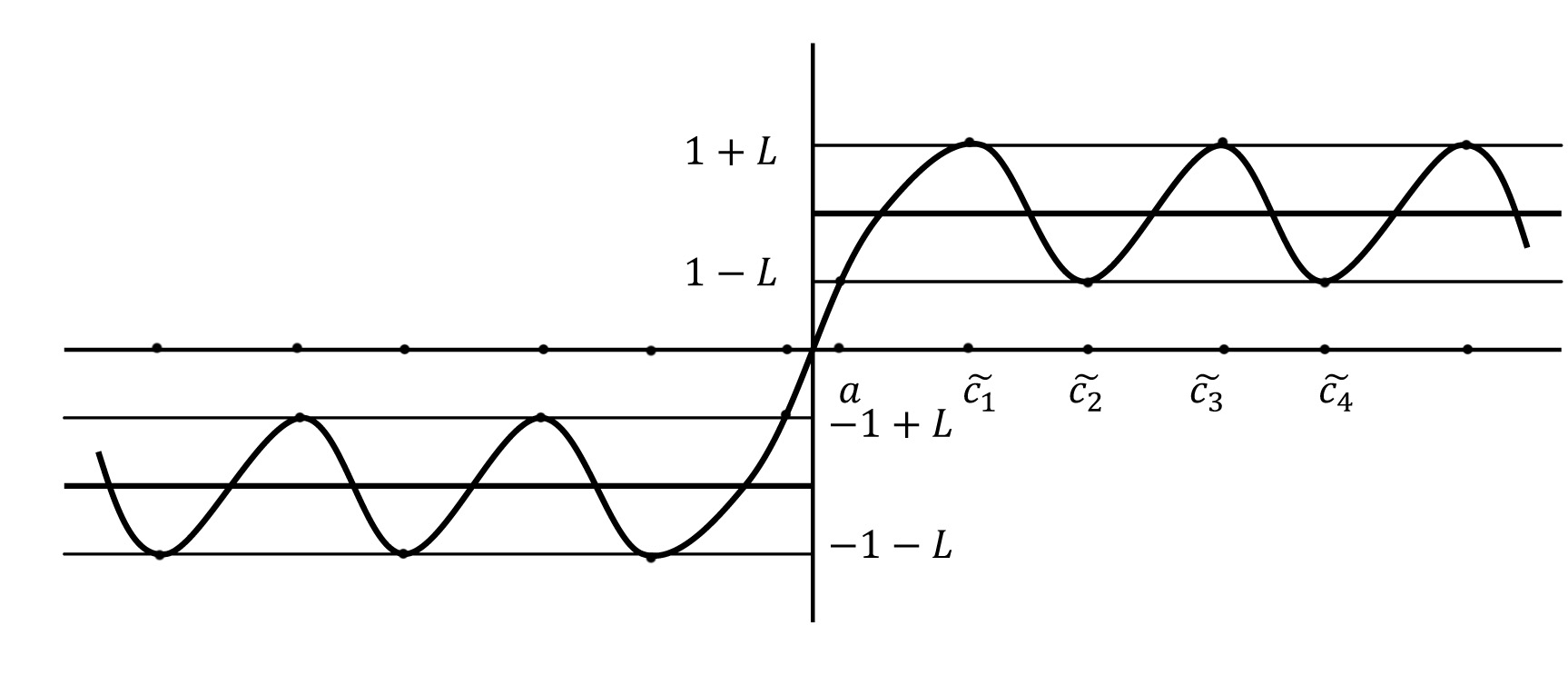
Figure 1: Graph of the function $\tilde{S}(z,a)$ on the real axis

We define the positive number $b=b(a)$ by $\cosh b=1/L(a)$. It is easy to see that $b$ is a continuous increasing function of $a$, and the correspondence $a\mapsto b$ is a homeomorphism of the positive ray onto itself.

For every $b>0$, we consider the region

$$\Omega=\{x+iy:x>0,y>0,x>\arccos(\cosh b/\cosh y)\;\mbox{for}\;y>b\}.$$

This region is shown in Fig. 2; it consists of the points in the first quadrant to the right of the curve

$$\gamma_{b}:=\{\arccos(\cosh b/\cosh t)+it:b\leq t<\infty\}.$$

Let $\tilde{\psi}$ be the conformal map of the first quadrant ${\mathbb{C}}_{++}$ onto $\Omega$, normalized by

$$\tilde{\psi}(z)=z+\dots,\ z\to\infty\ \text{and}\ \tilde{\psi}(0)=b.$$ (2.2)

Put $a=\tilde{\psi}^{-1}(0)$.

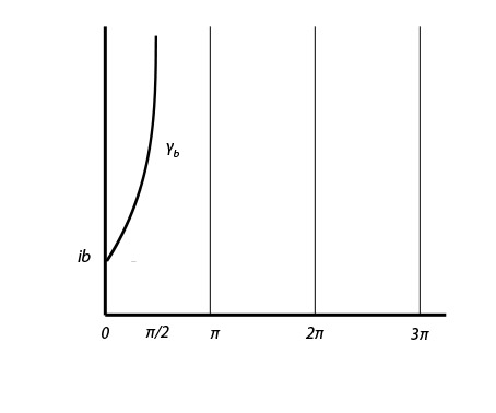
Figure 2: Domain $\Omega$ such that $\tilde{S}(z)=1-L(a)\cos\tilde{\psi}(z)$, $\tilde{\psi}:{\mathbb{C}}_{++}\to\Omega$.

In [5] we proved that

$$\tilde{S}(z,a)=1-L(a)\cos\tilde{\psi}(z),\quad z\in{\mathbb{C}}_{++}:=\{z:\text{\rm Re\ }z>0,\;\text{\rm Im\ }z>0\}.$$ (2.3)

As the right hand side of (2.3) takes real values on the positive ray and imaginary values on the positive imaginary ray, $\tilde{S}$ extends to the whole plane as an odd entire function.

The following asymptotics hold

$$\lim_{a\to\infty}\sqrt{a}e^{a}L(a)=\sqrt{\frac{2}{\pi}}.$$ (2.4)

Notice that all critical points $\{\pm\tilde{c}_{k}\}$ of $\tilde{S}(z,a)$ are real, and $\tilde{\psi}(\tilde{c}_{k})=\pi k$.

It is convenient to modify a little this conformal mapping. We write $S(z,a):=\tilde{S}(\sqrt{z^{2}+a^{2}},a)$, where $z$ belongs to the upper half-plane ${\mathbb{C}}_{+}$ with the slit $\{it:0<t\leq a\}$, see Fig. 3. Function $S$ is not entire, it is only defined in the upper half-plane.

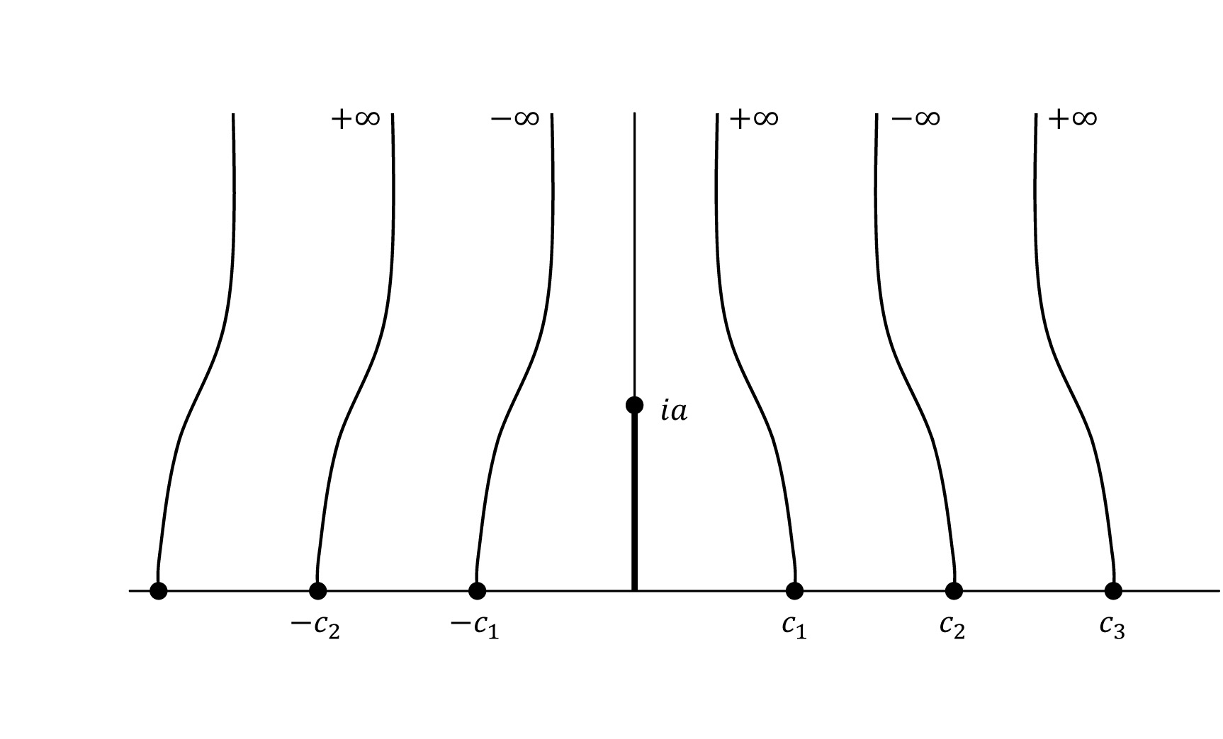
Figure 3: Preimage $S^{-1}({\mathbb{R}},a)$ in the upper half-plane

Again we have the conformal mapping $\psi:{\mathbb{C}}_{++}\to\Omega$ but in contrast with (2.2)

$$\psi(z)=z+\dots,\ z\to\infty,\ \ \psi(0)=0,$$ (2.5)

and therefore $\psi(ia)=ib$. The full preimage of the real axis under $S$ in the upper half-plane consists of the curves

$$\delta_{k}=\psi^{-1}(\{\pi k+it:t>0\}),\quad k=\pm 1,\pm 2,\ldots.$$ (2.6)

shown in Fig. 3. These curves have vertical asymptotes $\{\text{\rm Re\ }z=\pi k-\pi/2\}.$

Now let $P_{n}(z)$ be the best approximation of $\text{\rm sgn}(x)$ by polynomials of degree at most $n$ on two intervals $I=I_{-}\cup I_{+}$, $I_{\pm}\subset{\mathbb{R}}_{\pm}$. Using a linear transformation we may always assume that $I=[-A,-1]\cup[1,B]$.

Our goal is to obtain a representation for the extremal polynomial in the form of the composition

$$P_{n}(z)=S(\Theta_{n}(z),a_{n})$$ (2.7)

where $\Theta_{n}$ is the conformal mapping of the upper half-plane on a suitable “curved” comb-like region, and $a_{n}$ is an appropriate value of the parameter $a$.

First we give typical examples of the representation (2.7) and then show that these examples exhaust all possibilities.

First example. For $n=4$, consider the following region $\Pi_{2,3}$, see Fig. 4. Its boundary consists of the vertical segment $[0,ia]$, the horizontal segment $[-c_{2},c_{3}]$ and the curves $\delta_{-2},\delta_{3}$.

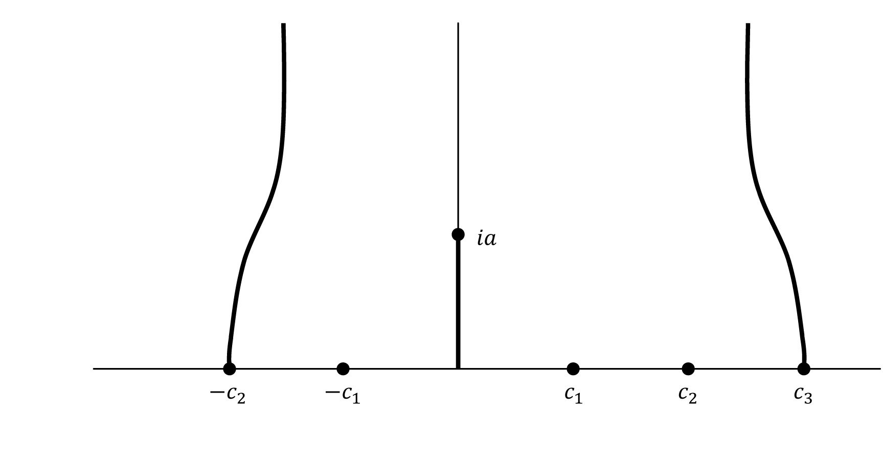
Figure 4: Domain $\Pi_{2,3}$

Let $\Theta(z)=\Theta_{4}(z)$ be the conformal mapping

$$\Theta:{\mathbb{C}}_{+}=\{z\in{\mathbb{C}},\ \text{\rm Im\ }z>0\}\to\Pi_{2,3},\quad\Theta(\pm 1)=0,\ \Theta(\infty)=\infty.$$ (2.8)

The function $P(z)=S(\Theta(z),a)$ can be extended to the lower half-plane due to the symmetry principle. Therefore it is an entire function, which is, in fact, a polynomial of degree $4$ due to its asymptotics at infinity. The graph of this polynomial on the real axis is of the form given in Fig. 5,

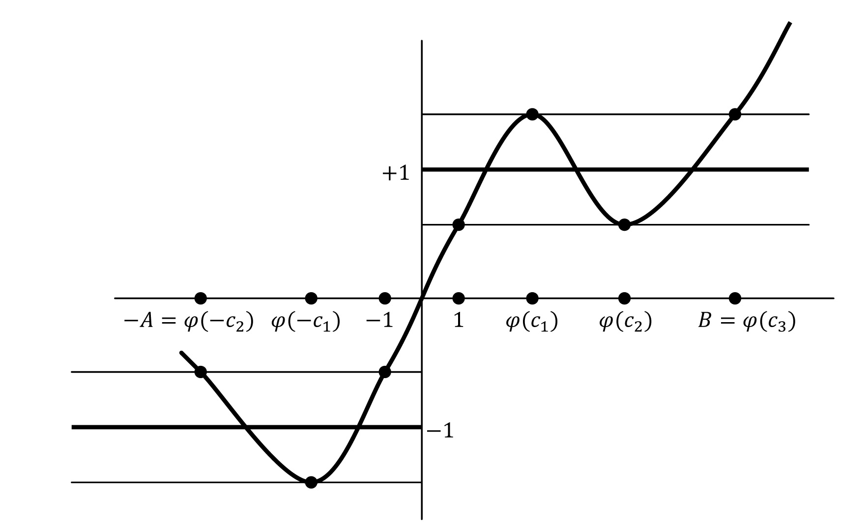
Figure 5: Extremal polynomial corresponding to the region $\Pi_{2,3}$

where $\phi=\Theta^{-1}$. By the Chebyshev theorem (for the two interval version of this theorem see [1], [2] [3]), $P(z)$ is the extremal polynomial on the set $I$ with $A=-\phi(-c_{2}),$ and $B=\phi(c_{3})$.

Second example. Let us point out that the above polynomial $P(z)$ has $7$ points of alternance, instead of $6$, which are required by the Chebyshev theorem for a polynomial of degree $4$. Therefore the same polynomial is extremal on the sets of two kinds

$$I=[-A,-1]\cup[1,\phi(c_{3})],\quad\phi(-c_{2})<-A\leq\phi(-c_{1})$$ (2.9)

or

$$I=[\phi(-c_{2}),-1]\cup[1,B],\quad\phi(c_{2})\leq B\leq\phi(c_{3}).$$ (2.10)

Third example. From the position $I=[\phi(-c_{2}),-1]\cup[1,\phi(c_{2})]$ we can start a deformation of the set $I$ and of the extremal polynomial. Namely consider the region $\Pi^{+}_{2,3}(h)$, see Fig. 6.

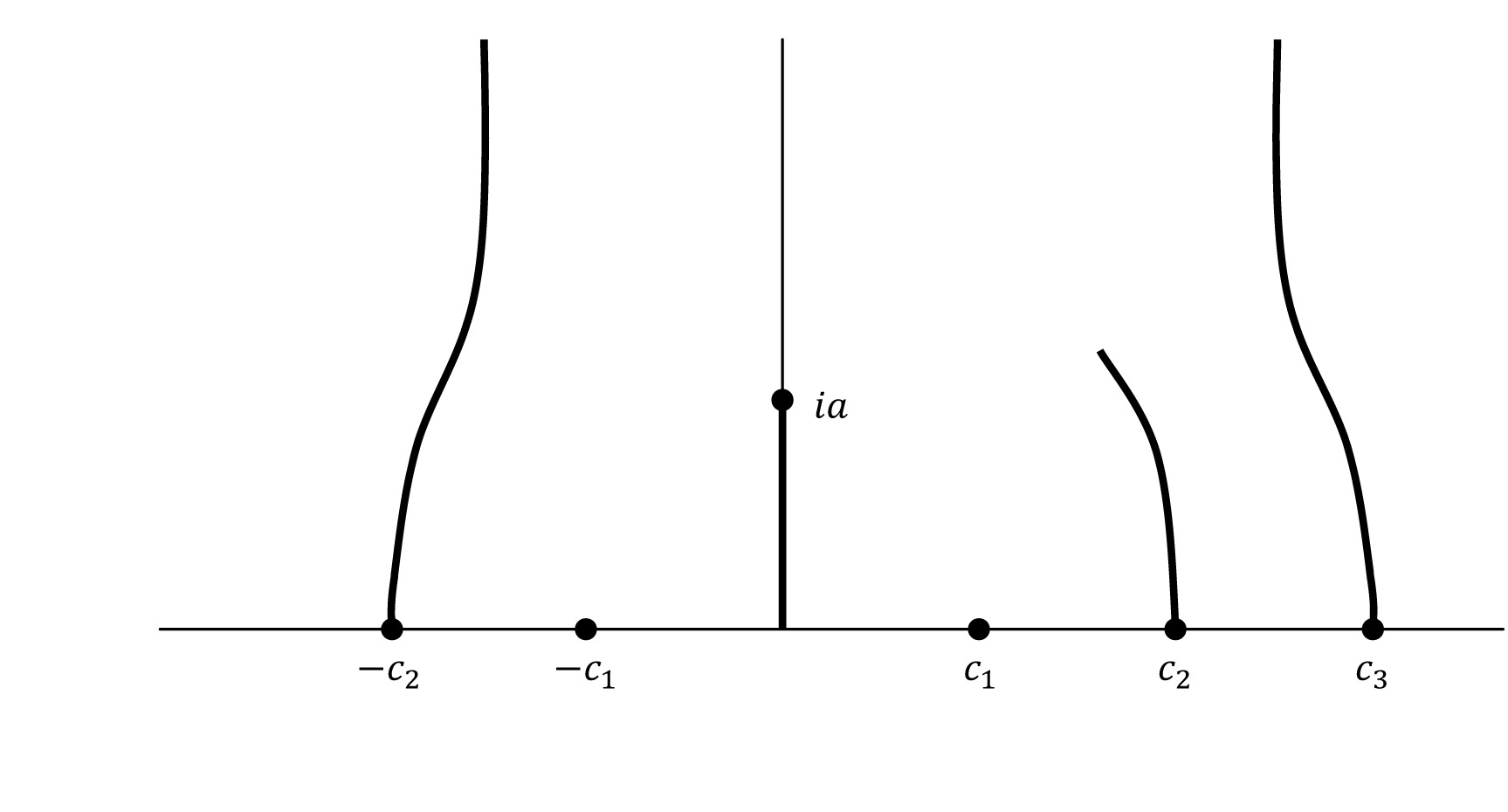
Figure 6: Domain $\Pi^{+}_{2,3}(h)$

Here we added to the boundary a segment of the curve $\delta_{2}$ that starts at the critical point $c_{2}$ and has length $h\in(0,\infty)$. In this case

$$\Theta:{\mathbb{C}}_{+}=\{z\in{\mathbb{C}},\ \text{\rm Im\ }z>0\}\to\Pi^{+}_{2,3}(h),\quad\Theta(\pm 1)=0,\ \Theta(\infty)=\infty,$$ (2.11)

and $P(z):=S(\Theta(z),a)$ is of the form given in Fig. 7.

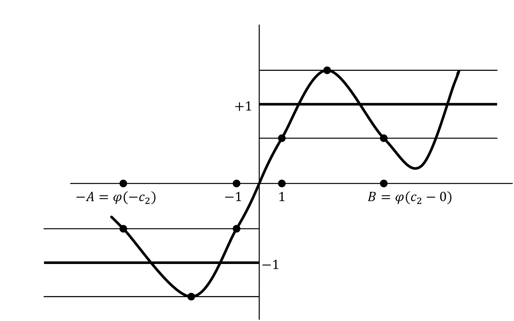
Figure 7: …and the corresponding extremal polynomial

For this new family of regions, which we parametrized by positive $h$, the polynomial is extremal on the set $I=[\phi(-c_{2}),-1]\cup[1,\phi(c_{2}-0)]$.

In the next section we show that these examples exhaust all possibilities for the extremal polynomials.

3 Parametrization

We begin with a general description of extremal polynomials. Fix $a>0$. This defines the number $L=L(a)$ and the function $S(\cdot,a)$. Let $k_{1}$ and $k_{2}$ be two positive integers. Consider the region $\Pi_{k_{1},k_{2}}$ in the upper half-plane bounded by the curves $\delta_{-k_{1}}$ and $\delta_{k_{2}}$. Then for $h\geq 0$ and $k_{2}\geq 2$, we define the region $\Pi_{k_{1},k_{2}}^{+}(h)$ by making in $\Pi_{k_{1},k_{2}}$ a slit along $\delta_{k_{2}-1}$ starting from $c_{k_{2}-1}$ and such that the length of its image under $\psi$ is $h$. So $\Pi^{\pm}_{k_{1},k_{2}}(0)=\Pi_{k_{1},k_{2}}$. Similarly we define $\Pi_{k_{1},k_{2}}^{-}(h)$ for $k_{1}\geq 2$ by making a slit along $\delta_{-k_{1}+1}$.

Let $\Theta$ be the conformal map of the upper half-plane onto $\Pi_{k_{1},k_{2}}^{+}(h)$, normalized by $\Theta(\pm 1)=0,\;\Theta(\infty)=\infty$. Consider the function

$$P(z)=S(\Theta(z),a).$$ (3.1)

By construction, it is real on the real line, so the symmetry principle implies that $P$ extends to an entire function. By looking at the asymptotic behavior as $z\to\infty$ we conclude that $P$ is a polynomial of degree $k_{1}+k_{2}-1$. All critical points of this polynomial are real. If $h=0$, then all critical values are $-1\pm L$ and $1\pm L$ on the negative and positive rays respectively. If $h>0$, the extreme left critical value is changed to $-1\pm L\cosh h$, or the extreme right critical value is changed to $1\pm L\cosh h$.

We have seen in the previous section that each of these polynomials $P$ is the extremal polynomial for some $A$ and $B$. Now we prove that for every $A$ and $B$ one of these polynomials is extremal.

Proposition 3.1.

All extremal polynomials are of the form (3.1) with $\Theta$ as defined above and some $k_{1},k_{2},a$ and $h$.

We give an elementary proof of this proposition, which is based on counting critical points and alternance points. This proof does not extend to the case of entire functions, so in Section 9 we will give another proof which is less elementary but avoids counting.

Proof.

In the proof we will use the following fact which is well-known and easy to prove.

Let $P_{1}$ and $P_{2}$ be two real polynomials with all critical points real and simple, and suppose that their critical points are listed in increasing order as $c_{1}<c_{2}<\ldots<c_{n-1}$ and $c_{1}^{\prime}<c_{2}^{\prime}<\ldots<c_{n-1}^{\prime}.$ If $P_{1}(c_{j})=P_{2}(c_{j}^{\prime})$ for $1\leq j\leq n-1$, then $P_{1}(z)=P_{2}(cz+b)$ for some $c>0$ and real $b$.

For a discussion and generalizations of this fact to entire functions, see [10], [12].

Let $A>1,B>1$, and a positive integer $n$ be given. (We will deal with the degenerate case $A=1$ or $B=1$ later). Let $P$ be the extremal polynomial of degree $n$ which exists and is unique by Chebyshev’s theorem. According to Chebyshev’s “alternance theorem”, this polynomial $P$ is characterized by the following properties: let $Q(x)=P(x)-\text{\rm sgn}(x)$, then

$$|Q(x)|\leq L,\quad x\in[-A,-1]\cup[1,B],$$ (3.2)

and there exist

$$m\geq n+2$$ (3.3)

points $x_{1}<x_{2}<\ldots<x_{m}$ in $[-A,-1]\cup[1,B]$ such that

$$|Q(x_{j})|=L,\quad 1\leq j\leq m,\quad\mbox{and}\quad Q(x_{j})Q(x_{j+1})<0,\quad 1\leq j\leq m-1.$$ (3.4)

These points $x_{j}$ are called the alternance points. Evidently, all alternance points in $(-A,-1)\cup(1,B)$ are critical, that is, $P^{\prime}(x)=0$ at all such points. Let $K$ be the number of critical alternance points and $N$ the number of non-critical alternance points. We have the evident inequalities

$$K\leq n-1\quad\mbox{and}\quad N\leq 4.$$

Combined with (3.3) this gives

$$n+2\leq m=K+N\leq n+3.$$

So we have three possibilities:

a) $m=n+3,\;N=4,\;K=n-1$. The last two equalities imply that all critical points of $P$ are real and simple, and each of them is an alternance point which belongs to $(-A,-1)\cup(1,B)$. All $4$ points $-A,-1,1,B$ are non-critical alternance points. So the graph has the shape shown in Fig. 5.

b) $m=n+2,\;N=3,\;K=n-1$. Again all critical points are real, simple, belong to $[-A,-1]\cup[1,B]$, and each critical point is an alternance point. All endpoints $-A,-1,1,B$ except possibly one are alternance points. Let us show that $-1$ and $1$ are alternance points.

Proving this by contradiction, suppose, for example that $-1$ is not an alternance point. Then $1$ cannot be a critical point because $N=3$. Thus $P^{\prime}(x)\neq 0$ on $[-1,1]$ and $P(1)\geq 1-L>-1+L\geq P(-1)$, we conclude that $P$ is strictly increasing on an interval $(-1-\epsilon,1+\epsilon)$ for some $\epsilon>0$. This implies that $1$ is also not an alternance point, a contradiction.

Thus the polynomial $P$ is of the type described in (2.9), (2.10).

c) $m=n+2,\;K=n-2,\;N=4$. In this case we have exactly one simple critical point $z$ which is not an alternance point. Evidently this exceptional critical point is real. We claim that it belongs to ${\mathbb{R}}\backslash[-A,B]$.

First of all, $z\notin\{-A,-1,1,B\}$ because $N=4$ so all these $4$ points are non-critical. Second, $z$ cannot be in the interior of one of the intervals $(-A,-1)$ or $(1,B)$. Indeed, if it is in the interior of one of these intervals, consider the adjacent alternance points $x_{j}$ and $x_{j+1}$ on the same interval such that $x_{j}<z<x_{j+1}$. Such $x_{j}$ and $x_{j+1}$ exist because all endpoints of each interval are alternance points, and $z$ is not an alternance point. As $z$ is the unique critical point on $(x_{j},x_{j+1})$, we obtain a contradiction with the alternance condition (3.4). Finally we prove that $z\notin(-1,1)$, Proving this by contradiction, suppose that $z\in(-1,1)$. As $-1$ is an alternance point we have $P(-1)=-1\pm L$. Suppose first that

$$P(-1)=-1-L.$$ (3.5)

Then $P^{\prime}(-1)<0$ because $-1$ is not critical ($N=4$ in the case we consider now), and (3.2) implies that $P^{\prime}(-1)\leq 0$. As $P^{\prime}$ changes sign exactly once on $(-1,1)$ and the point $1$ is also non-critical, we conclude that $P^{\prime}(1)>0$. As $P(1)=1\pm L$, (3.2) implies $P(1)=1-L$. This equality and (3.5) contradict the alternance condition (3.4). The case $P(-1)=-1+L$ is considered similarly.

Let $c$ be the critical point which is outside $[A,B]$. It is easy to see that $|P(c)+1|>L$ if $c<0$ and $|P(c)-1|>L$ if $c>0$. This is because $N=4$ and thus $A$ and $B$ are non-critical alternance points.

So in the case c) we have the graph of the type shown in Fig 7.

To summarize, we proved that in all cases the critical points are real and simple, all critical values, with at most one exception are $-1\pm L$ on the negative ray and $1\pm L$ on the positive ray, and the exceptional critical value, if it exists, corresponds to an extreme (left or right) critical point. If the exceptional critical point $c$ is positive then $|P(c)-1|>L$ and if $c$ is negative then $|P(c)+1|>L$.

Polynomials $S(\Theta,a)$ constructed above permit to match any such critical value pattern, so we conclude that $P(z)=S(\Theta(cz+b),a)$ with $c>0$ and $b\in{\mathbb{R}}$. Finally, the points $-1,1$ are always non-critical alternance points, and this implies that $c=1$ and $b=0$.

It remains to consider the degenerate case. Suppose, for example that $B=1$. Then only $3$ alternance points can be non-critical, so we are in the case b). The extremal polynomial in this degenerate case can be easily written explicitly:

$$P_{n}(x)=L_{n}T_{n}\left(\frac{2x+A+1}{A-1}\right)-1,$$

where $T_{n}(x)=\cos n\arccos x$, and

$$L_{n}=\frac{2}{T_{n}(1+4/(A-1))+1}\sim 4\exp\left(-n\operatorname{ch}^{-1}\left(1+\frac{4}{A-1}\right)\right)$$

is the approximation error. ∎

Remarks. It is easy to see that our polynomials depend continuously on $h$. When $h\to\infty$, we have $\Pi_{k_{1},k_{2}}^{+}(h)\to\Pi_{k_{1},k_{2}-1}$ and $\Pi_{k_{1},k_{2}}^{-}(h)\to\Pi_{k_{1}-1,k_{2}}$ in the sense of Caratheodory, and the corresponding polynomials converge uniformly on compact subsets of the plane.

Let us show that $A(h)$ and $B(h)$ depend monotonically on $h$. Let $h>h_{1}$, $\Theta(z)=\Theta(z,h)$ and $\Theta_{1}(z)=\Theta(z,h_{1}).$ Then the function $w(z)=\Theta_{1}^{-1}\circ\Theta(z)$ maps the upper half-plane into itself, and has the properties: $w(\pm 1)=\pm 1,w(\infty)=\infty.$ Thus it has a representation

$$w(z)=\rho_{\infty}(z-1)+1+\int\frac{z-1}{(x-1)(x-z)}d\rho(x)$$

where $d\rho$ is positive and supported on a compact set $I$ such that $x>B$ for all $x\in I$, and $\rho_{\infty}>0$. Here we used $w(1)=1$ and $w(\infty)=\infty$. Now we use the condition $w(-1)=-1$. We obtain

$$\rho_{\infty}=1-\int\frac{1}{(x-1)(x+1)}d\rho(x)$$ (3.6)

Since $w(B)=B_{1}$ we have

$$B_{1}-B=(\rho_{\infty}-1)(B-1)+(B-1)\int\frac{1}{(x-1)(x-B)}d\rho(x).$$

Using (3.6) we get

$$B_{1}-B=(B-1)\int\frac{B+1}{(x-1)(x-B)(x+1)}d\rho(x)>0.$$

Similarly

$$-A_{1}+A=(A+1)\int\frac{A-1}{(x-1)(x+A)(x+1)}d\rho(x)>0.$$

4 Integral representations

Asymptotic relations for the extremal polynomials are based on an integral representation of the conformal map $\Theta$.

Consider the conformal map of $\overline{\mathbb{C}}\backslash I$ onto on the annulus in Fig. 8.

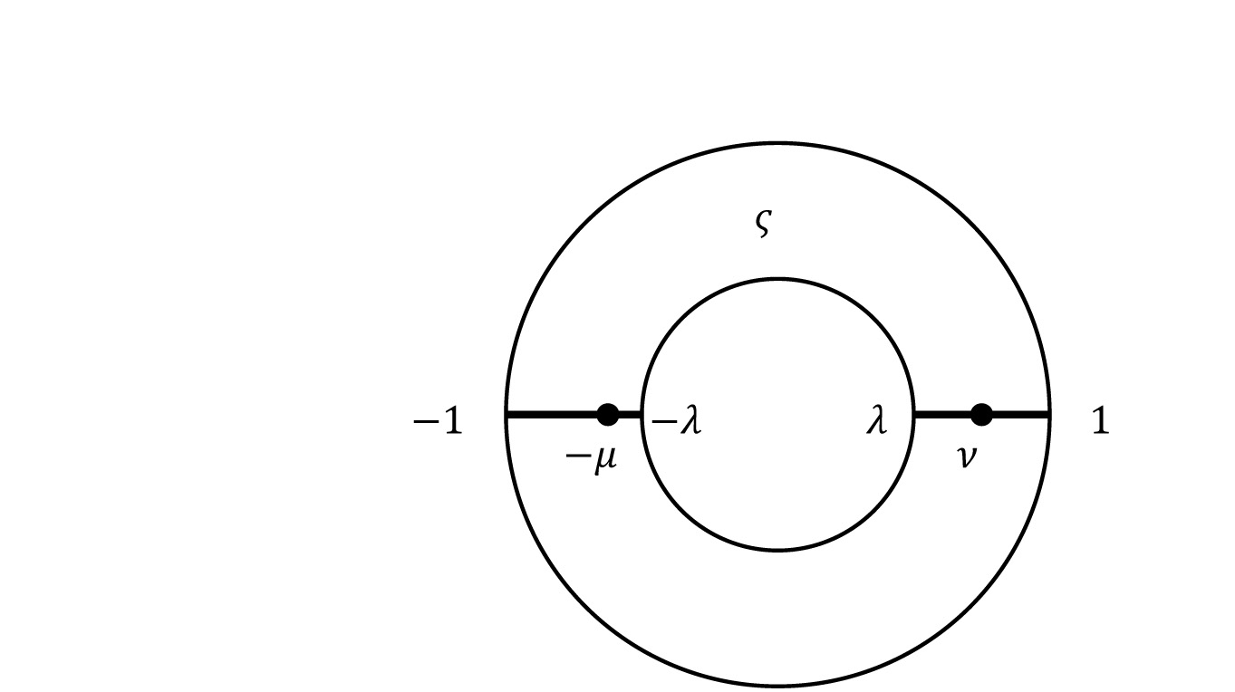
Figure 8: The conformally equivalent annulus.

Here we assume that the upper half-plane is mapped on the upper part of the annulus with the following boundary correspondence

$$B\mapsto-1,\ -A\mapsto-\lambda,\ -1\mapsto\lambda,\ 1\mapsto 1.$$ (4.1)

By $G(z,z_{0})$ we denote the (real) Green function of the region $\bar{\mathbb{C}}\setminus I$, $I=[-A,-1]\cup[1,B]$, with pole at $z_{0}$. In particular $G(z):=G(z,\infty)$. Recall that in the upper half-plane $G(z)$ can be represented as the imaginary part of the conformal mapping $\Phi(z)$ of the upper half-plane onto the region $\Pi$, Fig 9:

$$G(z)=\text{\rm Im\ }\Phi(z),\ \text{\rm Im\ }z>0,\ \Phi(\pm 1)=0,\ \Phi(\infty)=\infty.$$ (4.2)

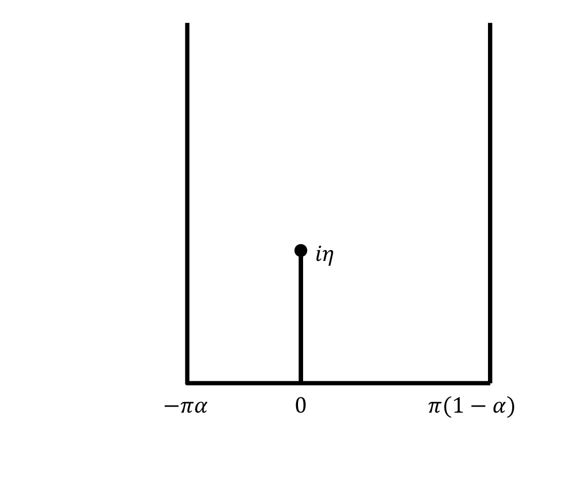
Figure 9: The image $\Pi$ of the map $\Phi$.

The map $\Phi(z)$ defines certain important characteristics of the region: the critical value

$$\eta=G(C),\quad C\in[-1,1]\quad\text{such that}\quad\nabla G(C)=0,$$ (4.3)

and the harmonic measure $\omega(z)$ of the interval $[-A,-1]$. We have

$$\Phi(-A)=-\pi\alpha,\quad\mbox{where}\quad\alpha=\omega(\infty).$$ (4.4)

Now we associate to $\Phi(z)$ the function

$$g(\zeta)=-i\Phi(z(\zeta))$$ (4.5)

where $\zeta$ belongs to the upper half of the annulus, see Fig. 8. This function can be extended to the upper half-plane by the symmetry principle. We have $G(z(\zeta))=\text{\rm Re\ }g(\zeta)$. We call $g$ the complex Green function.

Let $-\mu\in[-1,-\lambda]$ corresponds to the infinity in the $z$-plane, $-\mu=\zeta(\infty)$ (see Fig. 8). We define the jump function

$$j(\xi)=\begin{cases}1,&\xi\in(-1,-\mu)\\ 0,&\xi\in(-\mu,-\lambda)\end{cases}$$ (4.6)

which we extend by the symmetry $j(1/\xi)=j(\xi)$, $j(\lambda^{2}\xi)=j(\xi)$ on the whole negative ray. Since

$$\text{\rm Im\ }g(\xi)=\left\{\begin{array}[]{ll}0,&\xi>0,\\ \pi\alpha,&\xi\in(-\mu,-\lambda),\\ \pi(\alpha-1),&\xi\in(-1,-\mu),\end{array}\right.$$

we obtain the following integral representation for $g(\zeta)$ in the upper half-plane

$$g(\zeta)=\int_{-\infty}^{0}\left\{\frac{1}{\xi-\zeta}-\frac{1}{\xi-1}\right\}(\alpha-j(\xi))d\xi.$$ (4.7)

Remark. In the representation (4.7) the normalization condition $\Phi(1)=0$ was used. The second normalization condition $\Phi(-1)=0$ gives

$$\alpha=\overline{j}:=\frac{\int_{-\infty}^{0}\left\{\frac{1}{\xi-\lambda}-\frac{1}{\xi-1}\right\}j(\xi)d\xi}{\int_{-\infty}^{0}\left\{\frac{1}{\xi-\lambda}-\frac{1}{\xi-1}\right\}d\xi}.$$

In what follows we will use the bar over a function to denote similar averages.

Naturally we can simplify (4.7), but the point is that we can write a similar representation for the conformal mapping $\Theta_{n}(z)$. Recall that for a given $n$, there exists a unique region $\Pi(n)=\Pi^{\pm}_{k_{1}(n),k_{2}(n)}(h_{n})$, see Fig. 6, such that the conformal mapping $\Theta_{n}:{\mathbb{C}}_{+}\to\Pi(n)$ represents the extremal polynomial (2.7). We define the function

$$\theta_{n}(\zeta)=-i\Theta_{n}(z(\zeta)),\quad\theta_{n}(\lambda^{2}\zeta)=\theta_{n}(\zeta).$$ (4.8)

We write the imaginary part of $\theta_{n}(\xi)$, $\xi<0$ as a sum

$$\text{\rm Im\ }\theta_{n}(\xi)=\pi k_{1}(n)-\frac{\pi}{2}+\pi nj(\xi)+\chi_{n}(\xi),$$ (4.9)

so that $\chi_{n}(\xi)$ is a continuous function, which is normalized by the condition $\chi_{n}(-\mu)=0$. Then

$$\theta_{n}(\zeta)=\frac{1}{\pi}\int_{-\infty}^{0}\left\{\frac{1}{\xi-\zeta}-\frac{1}{\xi-1}\right\}(\pi k_{1}(n)-\frac{\pi}{2}-\pi nj(\xi)+\chi_{n}(\xi))d\xi.$$ (4.10)

Theorem 4.1.

In the above notations

$$\theta_{n}(\zeta)-ng(\zeta)=\frac{1}{\pi}\int_{-\infty}^{0}\left\{\frac{1}{\xi-\zeta}-\frac{1}{\xi-1}\right\}(\chi_{n}(\xi)-\bar{\chi}_{n})d\xi,$$ (4.11)

where

$$\bar{\chi}_{n}=\frac{\int_{-\infty}^{0}\left\{\frac{1}{\xi-\lambda}-\frac{1}{\xi-1}\right\}\chi_{n}(\xi)d\xi}{\int_{-\infty}^{0}\left\{\frac{1}{\xi-\lambda}-\frac{1}{\xi-1}\right\}d\xi}=\pi n\alpha-\pi k_{1}(n)+\frac{\pi}{2}.$$ (4.12)

Proof.

We subtract $ng(\zeta)$ in the form (4.7) from (4.11). Then, we use the second normalization condition $g(\lambda)=\theta_{n}(\lambda)=0$. ∎

This representation will imply Fuchs’ asymptotics as soon as we show that $\chi_{n}(\xi)$ is uniformly bounded.

5 Fuchs’ asymptotics

Let us begin with a simple remark.

Lemma 5.1.

Let $w(z)$ be a conformal mapping of the upper half-plane onto a sub-region of the upper half-plane which contains the half-plane $\text{\rm Im\ }w>\tau_{0}$. Assume the normalization $w(z)\sim z$, $z\to\infty$. Then

$$\text{\rm Im\ }w(z)-\text{\rm Im\ }z\in(0,\tau_{0}).$$ (5.1)

Proof.

Consider the integral representation of $\text{\rm Im\ }w(z)$

$$\text{\rm Im\ }w(z)=\text{\rm Im\ }z+\frac{1}{\pi}\int_{-\infty}^{\infty}P(z,t)v(t)dt,$$ (5.2)

where $P(z,t)$ is the Poisson kernel. Since $0\leq v(t)\leq\tau_{0}$ we obtain the desired inequality. ∎

Proposition 5.2.

There are constants $C_{1}$ and $C_{2}$ (depending of the given system of intervals $I$) such that

$$C_{1}\leq a_{n}-n\eta\leq C_{2}.$$ (5.3)

Proof.

Recall that the curves in Fig. 3 were defined as preimages of vertical lines in the region $\Omega$ in Fig. 2 under a conformal mapping which maps the right half-plane into a sub-region of the right half-plane. Thus we can apply Lemma 5.1, to obtain that $|\chi_{n}(\xi)|\leq 2\pi$. Therefore $|\chi_{n}(\xi)-\bar{\chi}_{n}|$ is also less than $2\pi$.

Now, $a_{n}$ is the maximum of $\theta_{n}(\xi)$ on the interval $(\lambda,1)$ and $\eta$ is the maximum of $g(\xi)$ on the same interval. Due to the integral representation (4.11) the difference between these two functions is uniformly bounded in this interval. Thus (5.3) is proved. ∎

Corollary 5.3.

The following limit relation holds

$$\lim_{n\to\infty}\frac{\theta_{n}(\zeta)}{n}=g(\zeta),$$ (5.4)

in particular

$$\lim_{n\to\infty}\frac{k_{1}(n)}{n}=\alpha,\quad\lim_{n\to\infty}\frac{\ln(1/L_{n})}{n}=\lim_{n\to\infty}\frac{a_{n}}{n}=\eta.$$ (5.5)

Proof.

We divide (4.11) by $n$ and pass to the limit. ∎

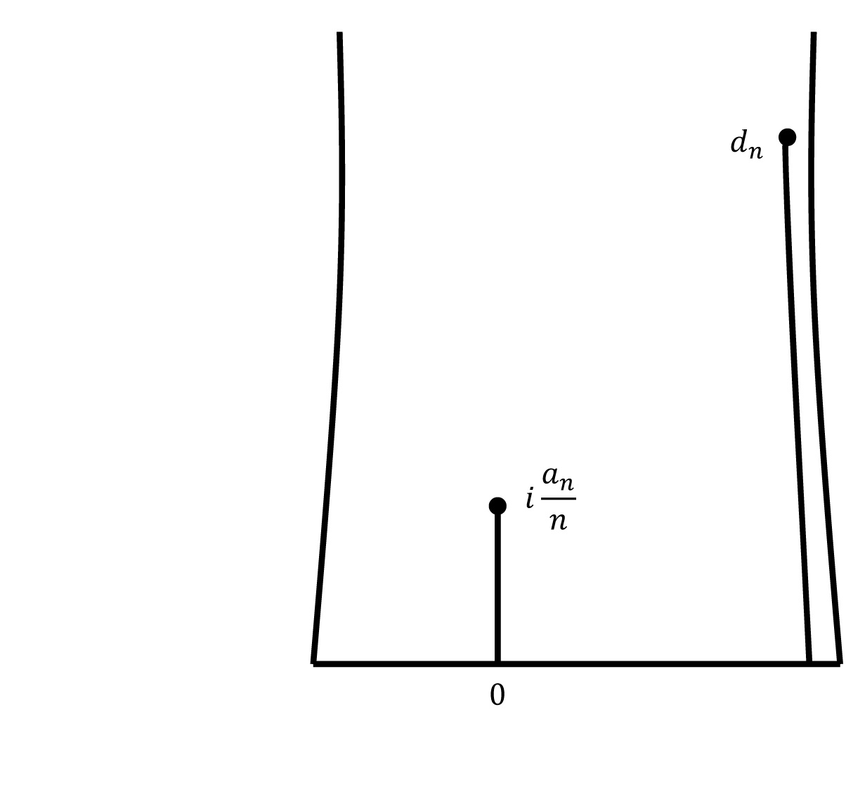
Figure 10: The rescaled region $\Pi(n)/n$ for a large $n$.

Corollary 5.3 has the following geometric interpretation. Making the rescaling $\Pi(n)\to\Pi(n)/n$ we obtain the limit conformal mapping onto the region shown in Fig. 9. Let us look more carefully at the limit procedure, see Fig 10: the distance between the additional cut and one of the infinite cuts (left or right one) approaches zero, however the position $d_{n}$ of the end point of the additional cut influences the asymptotic behavior along various subsequences $\{n_{l}\}$. We define the subsequences by the condition: there exists a limit $d=d(\{n_{l}\})=\lim_{l\to\infty}d_{n_{l}}$. Taking into account this point $d$, in the next section we describe the asymptotic behavior of $L_{n}$ in a more precise way.

6 The limit density $\chi(\xi)$

We fixed a subsequence $\{n_{l}\}$ such that the limit $d=\lim_{l\to\infty}d_{n_{l}}$ exists. Our main goal in this section is to show that the limit density

$$\chi(\xi)=\lim_{l\to\infty}\chi_{n_{l}}(\xi)$$ (6.1)

exists and to find this limit.

We start with the following general lemma. Let $f$, be a bounded increasing differentiable function defined for $x>0$, and suppose that $f(x)=0$ for $0<x\leq b$ with some $b>0$. We consider the region

$$\tilde{\Omega}_{f}=\{z=x+iy:x>0,\;y>f(x)\},$$ (6.2)

(it looks like the region $\Omega$ in Fig. 2 reflected in the line $x=y$). Let $w$ be the conformal map from the first quadrant ${\mathbb{C}}_{++}$ onto $\tilde{\Omega}_{f}$ with the normalization

$$w(z)\sim z,\ z\to\infty,\quad w(0)=0.$$ (6.3)

Let $a$ be the point such that $w(a)=b$.

Lemma 6.1.

Let $w(x)=u(x)+iv(x)$, $x\geq a$. Then $f(x)\leq v(x)$.

Proof.

We extend $w$ by the symmetry principle to the map of the upper half-plane into itself (the extended map is still denoted by $w$), and use the integral representation

$$w(z)=z+\frac{1}{\pi}\int_{a}^{\infty}\left\{\frac{1}{t-z}-\frac{1}{t+z}\right\}v(t)dt.$$ (6.4)

For $x\geq a$ we have

$$w(x)=x+\frac{1}{\pi}\int_{a}^{\infty}\frac{2x}{t+x}\frac{v(t)-v(x)}{t-x}dt+\frac{v(x)}{\pi}\ln\frac{x+a}{x-a}+iv(x).$$ (6.5)

Therefore

$$u(x)=x+\frac{1}{\pi}\int_{a}^{\infty}\frac{2x}{t+x}\frac{v(t)-v(x)}{t-x}dt+\frac{v(x)}{\pi}\ln\frac{x+a}{x-a}>x.$$ (6.6)

Since $f(x)$ is increasing we obtain

$$f(x)<f(u(x))=v(x).$$ (6.7)

∎

We apply Lemma 6.1 to obtain the limit density for the conformal map of the first quadrant onto the region $\Omega$ in Fig. 2. Namely, as before we consider the conformal map $w(z)=-i\psi(-iz)$, where $\psi$ is defined in (2.5) and extended by symmetry to the right half-plane, and the integral representation (6.4) for it. Let us notice that in our case we have the exact formula

$$f(x)=\arccos\frac{\cosh b}{\cosh x},\ x\geq b.$$ (6.8)

Between the values $a$ and $b$ there is a one-to-one correspondence, moreover $b\sim a+1/2\ln a$. Thus we have the density $v(x)=v(x,a)$ in (6.4) as a function of the parameter $a$ and we are interested in the limit density $\tilde{v}(x):=\lim_{a\to\infty}v(ax,a)$.

Lemma 6.2.

The following limit exists

$$\tilde{v}(x):=\lim_{a\to\infty}v(ax,a)=\begin{cases}0,&x<1\\ \frac{\pi}{2},&x>1.\end{cases}$$ (6.9)

Proof.

It is evident, that $\tilde{v}(x)=0$ for $x\in(0,1)$. For $x>1$ we use Lemma 6.1 and the asymptotic relation between $a$ and $b$:

$$v(ax,a)\geq\arccos\frac{\cosh b}{\cosh ax}\sim\arccos\frac{\sqrt{a}}{e^{(x-1)a}}.$$ (6.10)

On the other hand $v(ax,a)\leq\pi/2$, thus the lemma is proved. ∎

Now we are in position to evaluate the limit density (6.1).

Theorem 6.3.

Let $\{n_{k}\}$ be a subsequence such that $\lim d_{n_{k}}=d$. Without loss of generality, we assume that $\text{\rm Re\ }d=\pi(1-\alpha)$ (alternatively $\text{\rm Re\ }d=\pi\alpha$). The relation

$$d=\Phi(D)=ig(-\kappa),$$ (6.11)

uniquely defines $D\in[B,\infty]$ and $-\kappa\in[-1,-\mu]$. Then

$$\chi(\xi)=\lim_{l\to\infty}\chi_{n_{l}}(\xi)=\begin{cases}\displaystyle\frac{1}{2}\int_{|t|<\eta}\frac{\pi\alpha}{(t-y)^{2}+(\pi\alpha)^{2}}dt,&-\mu<\xi<-\lambda,\\ \displaystyle\frac{1}{2}\int_{|t|<\eta}\frac{\pi(\alpha-1)}{(t-y)^{2}+(\pi(\alpha-1))^{2}}dt,&-\kappa<\xi<-\mu,\\ \displaystyle\frac{1}{2}\int_{|t|<\eta}\frac{\pi(\alpha-1)}{(t-y)^{2}+(\pi(\alpha-1))^{2}}dt+\pi,&-1<\xi<-\kappa,\\ \end{cases}$$ (6.12)

where $y=\text{\rm Re\ }g(\xi)$.

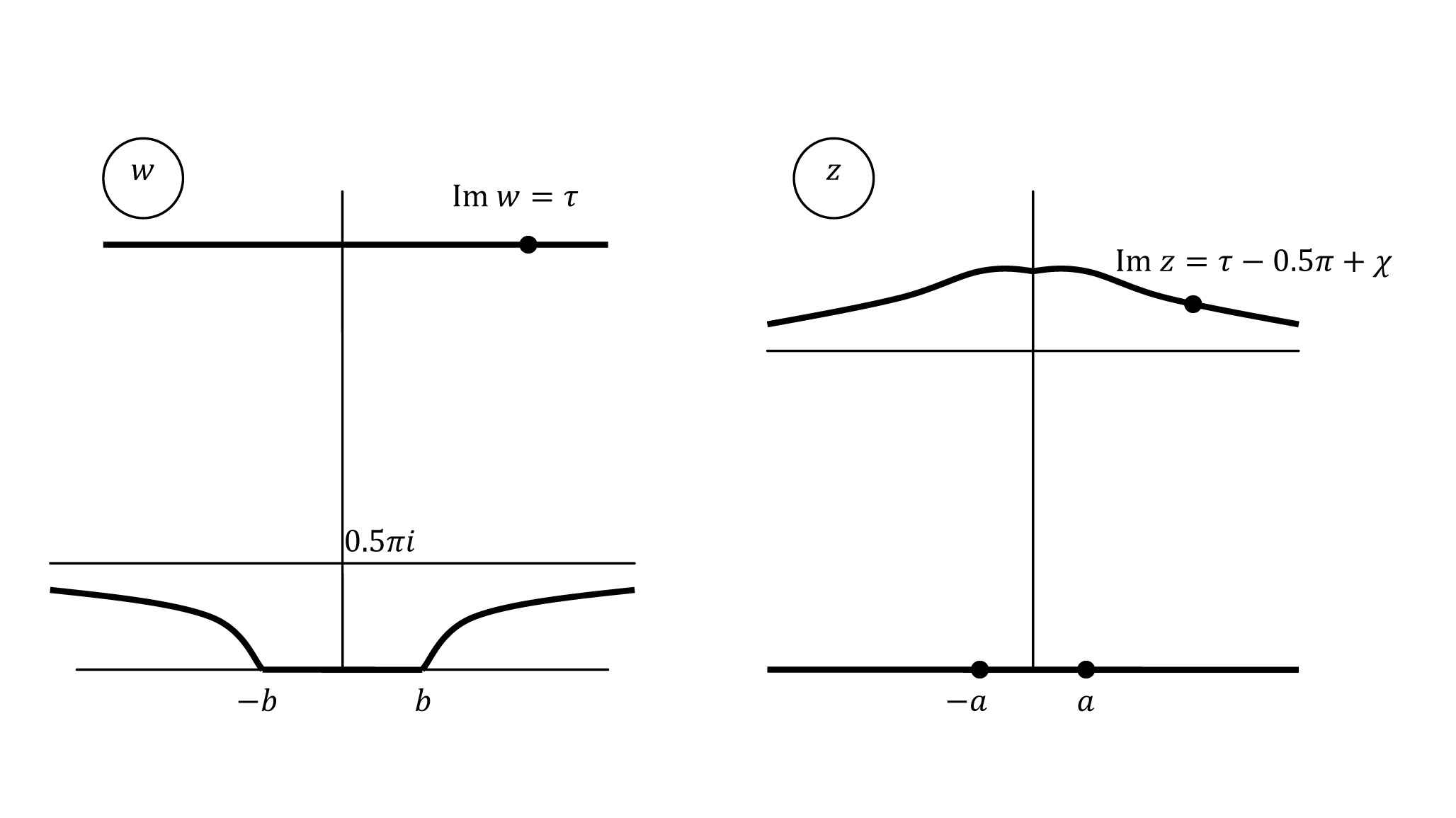
Figure 11: The preimage of the level line $\text{\rm Im\ }w=\tau$

Proof.

First we assume that $-\mu<\xi<-\lambda$. Let $z_{l}=\theta_{n_{l}}(\xi)$. For a sufficiently large $l$, by (6.4), we have

$$\text{\rm Im\ }w_{l}=\text{\rm Im\ }z_{l}+\frac{1}{\pi}\int_{|t|>a_{n_{l}}}\frac{\text{\rm Im\ }z_{l}}{(t-\text{\rm Re\ }z_{l})^{2}+\text{\rm Im\ }z_{l}^{2}}v(t,a_{n_{l}})dt.$$ (6.13)

Substituting $\text{\rm Im\ }z_{l}=\pi k_{1}(n_{l})-\frac{\pi}{2}+\chi_{n_{l}}(\xi)$ and $\text{\rm Im\ }w_{l}=\pi k_{1}(n_{l})$ to (6.13) (see Fig. 11) we obtain

$$\begin{split}\displaystyle\pi/2-\chi_{n_{l}}(\xi)=\displaystyle&\frac{1}{\pi}\int_{|t|>a_{n_{l}}}\frac{(\pi k_{1}(n_{l})-\pi/2+\chi_{n_{l}}(\xi))v(t,a_{n_{l}})}{(t-y_{l}(\xi))^{2}+(\pi k_{1}(n_{l})-\pi/2+\chi_{n_{l}}(\xi))^{2}}dt\\ \displaystyle=&\frac{1}{\pi}\int_{|t|>1}\frac{(\pi k_{1}(n_{l})-\pi/2+\chi_{n_{l}}(\xi))a_{n_{l}}v(a_{n_{l}}t,a_{n_{l}})}{(a_{n_{l}}t-y_{l}(\xi))^{2}+(\pi k_{1}(n_{l})-\pi/2+\chi_{n_{l}}(\xi))^{2}}dt\end{split}$$ (6.14)

By the leading term asymptotics, Corollary 5.3, we have

$$\lim_{l\to\infty}\frac{k_{1}(n_{l})}{n_{l}}=\alpha,\ \lim_{l\to\infty}\frac{a_{n_{l}}}{n_{l}}=\eta,\lim_{l\to\infty}\frac{y_{l}(\xi)}{n_{l}}=y(\xi).$$ (6.15)

Passing to the limit in (6.14) we get

$$\pi/2-\chi(\xi)=\frac{1}{\pi}\int_{|t|>1}\frac{\eta\pi\alpha}{(\eta t-y)^{2}+(\pi\alpha)^{2}}\tilde{v}(t)dt,$$ (6.16)

By Lemma 6.2, after trivial simplifications we obtain the first equation in (6.12).

In the second case $-\kappa<\xi<-\mu$, for sufficiently large $l$, the point $z_{l}$ corresponds to a point $w_{l}$ on the line $\text{\rm Im\ }w_{l}=\pi k_{2}(n_{l})$. Thus we can repeat the previous arguments with $\alpha$ replaced by $1-\alpha$ (let us mention that $\chi_{n_{l}}(\xi)$ is negative here).

In the last case $\text{\rm Im\ }w_{l}=\pi(k_{2}(n_{l})-1)$, and this leads to the shift of the limit value by $\pi$. ∎

7 Simplifying the result

In this section we prove the following theorem, which is our main result, and which implies Theorem 1.1.

Theorem 7.1.

Let $\nu$ be the point in the interval $(\lambda,1)$, such that $g(\nu)=\eta$. Fix a subsequence $\{n_{l}\}$ such that $\lim_{l\to\infty}{d_{n_{l}}}=d=ig(-\kappa)$. Let $g(\zeta,\nu)$ and $g(\zeta,-\kappa)$ be the corresponding complex Green functions. Then

$$\lim_{l\to\infty}\{\theta_{n_{l}}(\zeta)-n_{l}g(\zeta)\}=\frac{1}{2}\ln\frac{\eta-g(\zeta)}{\eta+g(\zeta)}+g(\zeta,\nu)-g(\zeta,-\kappa).$$ (7.1)

Proof. First of all we split $\chi(\xi)$ into the sum of a continuous function $\chi_{c}(\xi)$ and the jump

$$j_{1}(\xi)=\begin{cases}1,&\xi\in(-1,-\kappa)\\ 0,&\xi\in(-\kappa,-\lambda)\end{cases}$$ (7.2)

As usual the jump function is extended to the negative ray by the reflections $j_{1}(1/\xi)=j_{1}(\xi)$, $j_{1}(\lambda^{2}\xi)=j_{1}(\xi)$.

Note that the jump function is related to the Green function $G(z,D)$, compare (4.6) and (4.7). Since

$$\text{\rm Im\ }g(\xi,-\kappa)=\left\{\begin{array}[]{ll}0,&\xi>0,\\ \pi\omega(D),&\xi\in(-\kappa,-\lambda),\\ \pi(\omega(D)-1),&\xi\in(-1,-\kappa),\end{array}\right.$$

we obtain the following integral representation for $g(\zeta,-\kappa)$ in the upper half-plane

$$g(\zeta,-\kappa)=\int_{-\infty}^{0}\left\{\frac{1}{\xi-\zeta}-\frac{1}{\xi-1}\right\}(\bar{j}_{1}-j_{1}(\xi))d\xi,$$ (7.3)

where we use the notation $\bar{j}_{1}$ introduced in the Remark in Section 4. Notice that $G(z(\zeta),D)=\text{\rm Re\ }g(\zeta,-\kappa)$, and

$$\bar{j}_{1}=\omega(D).$$ (7.4)

Due to the chosen normalization $\chi(-\mu)=0$, we have

$$\chi(\xi)=\begin{cases}\chi_{c}(\xi)+\pi j_{1}(\xi),&-\kappa<-\mu\\ \chi_{c}(\xi)+\pi j_{1}(\xi)-\pi,&-\mu<-\kappa\end{cases}$$ (7.5)

The main point is to evaluate the Cauchy transform of the continuous part $\chi_{c}(\xi)$.

Lemma 7.2.

Let $\nu\in(\lambda,1)$ be such that $g(\nu)=\eta$, that is, $\nu$ corresponds to the critical point $C\in(-1,1)$. Let $g(\zeta,\nu)$ be the corresponding complex Green function. Then

$$\frac{1}{\pi}\int_{-\infty}^{0}\left\{\frac{1}{\xi-\zeta}-\frac{1}{\xi-1}\right\}(\chi_{c}(\xi)-\bar{\chi}_{c})d\xi=\frac{1}{2}\ln\frac{\eta-g(\zeta)}{\eta+g(\zeta)}+g(\zeta,\nu).$$ (7.6)

Proof.

Using (6.12), for $z=y(\xi)+i\alpha=g(\xi)$, $\xi\in(-\mu,-\lambda)$, we have

$$\chi_{c}(\xi)=\frac{1}{2}\text{\rm Im\ }\int_{-\eta}^{\eta}\frac{1}{t-z}dt=\frac{1}{2}\text{\rm Im\ }\ln\frac{\eta-z}{-\eta-z}.$$ (7.7)

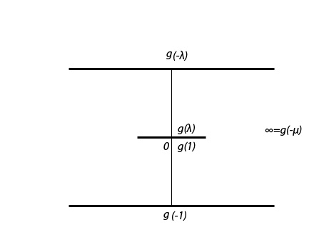
Figure 12: The image of the Green function

So let us consider the function

$$f(\zeta):=\frac{1}{2}\ln\frac{\eta-g(\zeta)}{-\eta-g(\zeta)}.$$ (7.8)

The image of the function $g(\zeta)$ is shown in Fig. 12, the image of the fraction linear transformation is shown in Fig. 13. Let us point out that for $\zeta$ in the upper half of the ring, Fig. 8, we obtain the values of $g(\zeta)$ in the right half-plane and for $\displaystyle\frac{\eta-g(\zeta)}{-\eta-g(\zeta)}$ in the unit disk. Thus,

$$\rho(\xi):=\text{\rm Im\ }f(\xi)=\begin{cases}\pi/2,&\lambda<\xi<\nu\\ -\pi/2,&\nu<\xi<1\end{cases}$$ (7.9)

here $\nu$ is such that $g(\nu)=\eta$.

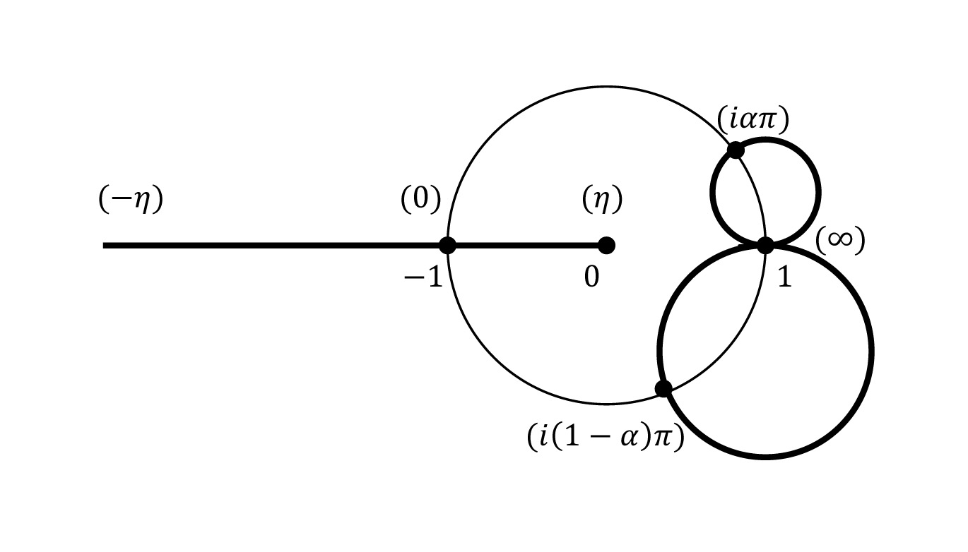
Figure 13: The image of $(\eta-g(\zeta))/(-\eta-g(\zeta))$

We use the integral representation of $f(\zeta)+i\pi/2$

$$\frac{1}{2}\ln\frac{\eta-g(\zeta)}{\eta+g(\zeta)}=f(\zeta)+\frac{\pi}{2}i=\frac{1}{\pi}\int_{-\infty}^{\infty}\left\{\frac{1}{\xi-\zeta}-\frac{1}{\xi-1}\right\}\left(\rho(\xi)+\frac{\pi}{2}\right)d\xi.$$ (7.10)

The complex Green function related to the critical point $C\in(-1,1)$ we still normalized by the condition $g(1,\nu)=0$. Therefore

$$\text{\rm Im\ }g(\xi,\nu)=\left\{\begin{array}[]{ll}-\pi,&\xi\in(\lambda,\nu),\\ -\pi(1-\omega(C)),&\xi<0,\\ 0,&\xi\in(\nu,1).\end{array}\right.$$

According to (7.9) we can represent $g(\zeta,\nu)$ as

$$\begin{split}g(\zeta,\nu)=&-(1-\omega(C))\int_{-\infty}^{0}\left\{\frac{1}{\xi-\zeta}-\frac{1}{\xi-1}\right\}d\xi\\ -&\frac{1}{\pi}\int_{0}^{\infty}\left\{\frac{1}{\xi-\zeta}-\frac{1}{\xi-1}\right\}\left(\rho(\xi)+\frac{\pi}{2}\right)d\xi.\end{split}$$ (7.11)

Recall that on the negative ray $\rho(\xi)=\chi_{c}(\xi)$, see (7.7). Adding (7.11) and (7.10) we obtain (7.6), moreover

$$\bar{\chi}_{c}=\pi(\frac{1}{2}-\omega(C)).$$ (7.12)

∎

Theorem 7.1 follows from Lemma 7.2, (4.11) and (7.3).

Completion of the proof of Theorem 1.1.

The error term $L_{n}$ satisfies

$$L_{n}\sim\sqrt{2/\pi}\,a_{n}^{-{1/2}}e^{-a_{n}},$$ (7.13)

where $a_{n}=\max\{\theta_{n}(\xi):\lambda<\xi<1\}.$ This follows from (2.4) and our explicit representation of the extremal polynomial (2.7).

The necessary constants $C,\eta,\eta_{1},\eta_{2},\alpha$ which depend only on $A$ and $B$, and the harmonic measure $\omega(x)=\omega(x,[-A,-1],\overline{\mathbb{C}}\backslash I)$ were defined in the Introduction.

According to (7.4), (7.12) and (7.5) we have

$$\frac{\bar{\chi}}{\pi}=\begin{cases}1/2-\omega(C)+\omega(D),&-\kappa<-\mu,\\ -1/2-\omega(C)+\omega(D),&-\mu<-\kappa.\end{cases}$$ (7.14)

Notice that $\omega$ is a strictly increasing function on ${\mathbb{R}}\backslash(-A,B)$ and the image of this set (together with the infinite point) equals $[0,1]$. Therefore, for every $n$ there exists a unique solution $D_{n}$ of the equation

$$\omega(D_{n})=\{\alpha n+\omega(C)\},$$ (7.15)

where $\{\cdot\}$ stands for the fractional part.

Equations (4.12), (7.14) and $d_{n_{l}}\to d$ imply that

$$\omega(D_{n_{l}})\to\omega(D).$$ (7.16)

Let $-\kappa_{n}\in(-1,-\lambda)$ be the point in $\zeta$-plane (see Fig. 8) which corresponds to $D_{n}$ in $z$-plane. Then $g(\zeta,-\kappa_{n_{l}})\to g(\zeta,-\kappa)$. Now (7.1) implies

$$\lim_{n_{l}\to\infty}(\theta_{n_{l}}(\zeta)-n_{l}g(\zeta)+g(\zeta,-\kappa_{n_{l}}))=\frac{1}{2}\ln\frac{\eta-g(\zeta)}{\eta+g(\zeta)}+g(\zeta,\nu).$$ (7.17)

The right hand side is independent of the subsequence $\{n_{l}\}$, so the limit as $n\to\infty$ exists in the left hand side. In the resulting formula we let $\zeta\to\nu$ and obtain

$$\lim_{n\to\infty}(\theta_{n}(\nu)-ng(\nu)+g(\nu,-\kappa_{n}))=-\frac{1}{2}\ln\frac{2\eta}{\eta_{1}}+\eta_{2}.$$ (7.18)

The functions $g(\zeta,-\kappa_{n})$ are uniformly bounded and have bounded derivatives on $(\lambda,1)$. Therefore,

$$a_{n}=\max\{\theta_{n}(\xi):\lambda<\xi<1\}=\theta_{n}(\nu)+o(1),\quad n\to\infty.$$

Thus

$$a_{n}=\eta n-G(D_{n},C)-\frac{1}{2}\ln\frac{2\eta}{\eta_{1}}+\eta_{2}+o(1).$$ (7.19)

To obtain the final result, this expression for $a_{n}$ has to be substituted to (7.13).

We can simplify the expression $e^{G(D_{n},C)}$ in the resulting formula and avoid solving equation (7.15) in the following way.

Let $F$ be the conformal map of the upper half-plane onto a rectangle $(0,p,p+i,i)$, where $p>0$ and the vertices of the rectangle correspond to $(1,B,-A,-1)$ in this order. It is easy to see that $\omega=\text{\rm Im\ }F$. So

$$F(C)=i\omega(C),$$ (7.20)

and in view of (7.15)

$$F(D_{n})=p+i\omega(D_{n})=p+i\{\alpha n+\omega(C)\}.$$ (7.21)

Christoffel–Schwarz formula gives (1.2), and $p=\tau/i,$ where $\tau$ is defined by (1.4). We reflect our rectangle with respect to the imaginary axis and apply the map $z\mapsto(i\pi/p)z$, to obtain the new rectangle

$$R=\{x+iy:-\pi/p<x<0,\;|y|<\pi\}.$$

Then $e^{z}$ maps this rectangle $R$ into a ring $e^{-\pi/p}<|w|<1$ and we use the expression of the Green function of this ring [3, §55 (4)] substituting to this formula $\ln w=i\pi-(\pi/p)\omega(D)$, $\ln c=(\pi/p)\omega(C)$ and using $\tau$ instead of $-1/\tau$. The result is simplified using Table VIII in [3] and we obtain

$$e^{G(D_{n},C)}=\left|\frac{\vartheta_{0}\left(\frac{1}{2}(\{n\omega(\infty)+\omega(C)\}-\omega(C))|\,\tau\right)}{\vartheta_{0}\left(\frac{1}{2}(\{n\omega(\infty)+\omega(C)\}+\omega(C))|\,\tau\right)}\right|,$$

where $\tau=ip$ is given by (1.4). Combining this with (7.13) and (7.19) we obtain the statement of Theorem 1.1.

8 Example (the symmetric case)

We consider the case $I=[-A,-1]\cup[1,A]$. In this case

$$G(z,\infty)=\int_{A}^{z}\frac{xdx}{\sqrt{(x^{2}-1)(x^{2}-A^{2})}}.$$ (8.1)

Therefore

$$\eta=\int_{0}^{1}\frac{xdx}{\sqrt{(x^{2}-1)(x^{2}-A^{2})}}=\frac{1}{2}\int_{1}^{\frac{A^{2}+1}{A^{2}-1}}\frac{dt}{\sqrt{t^{2}-1}}=\frac{1}{2}\ln\frac{A+1}{A-1}$$ (8.2)

and

$$\eta_{1}=-\frac{1}{2}G^{\prime\prime}(0,\infty)=\frac{1}{2A}.$$ (8.3)

Also,

$$G(z,0)=\int_{-1}^{z}\frac{Adx}{x\sqrt{(x^{2}-1)(x^{2}-A^{2})}}\sim\ln\frac{1}{z}+\ln\frac{2A}{\sqrt{A^{2}-1}}.$$ (8.4)

Notice that $\omega(\infty)=1/2$, $C=0$ and $\omega(C)=1/2$. Therefore for $n=2m+2$ we have $D_{n}=\infty$, so $L_{2m+2}=L_{2m+1}$.

For $n=2m+1$ we get

$$\begin{split}\sqrt{(2m+1)\eta}\sqrt{\frac{\eta_{1}}{2\eta}}e^{(2m+1)\eta+\eta_{2}}L_{2m+1}\\ \\ =\sqrt{\frac{2m+1}{4A}}\left(\frac{A+1}{A-1}\right)^{m}\sqrt{\frac{A+1}{A-1}}\frac{2A}{\sqrt{A^{2}-1}}L_{2m+1}.\end{split}$$ (8.5)

Finally,

$$\lim_{m\to\infty}\sqrt{2m+1}\left(\frac{A+1}{A-1}\right)^{m}\frac{\sqrt{A}}{A-1}L_{2m+1}=\sqrt{\frac{2}{\pi}},$$ (8.6)

as we proved in [5].

9 Approximation of $\text{\rm sgn}(x)$ by entire functions on $[-A,-1]\cup[1,+\infty)$

Only a minor variation of our method is needed to investigate the following problem: minimize

$$\sup\{|f(x)-\text{\rm sgn}(x)|:x\in[-A,-1]\cup[1,+\infty)\}$$ (9.1)

among all entire functions $f$ of order $1/2$, type $\sigma$.

Let $E(\sigma)$ be the infimum (9.1). It is easy to prove the existence of an extremal function using normal families arguments.

Now we describe a construction of extremal functions. We take the error $E$ as an independent parameter. Let $a>0$ be the unique solution of the equation $L(a)=E$, where $L(a)$ is defined in the beginning of Section 2. For $h\geq 0$, and an integer $k\geq 2$, let $\Pi_{k}(h)=\Pi^{-}_{k,\infty}(h)$, that is the region in the upper half-plane whose boundary with respect to the upper half-plane consists of the segment $[0,ia]$, and the curve $\delta_{-k}$ as in (2.6). Let $\Theta_{k,h}:{\mathbb{C}}_{+}\to\Pi_{k}(h)$ be the conformal map normalized by $\Theta_{k,h}(\pm 1)=0,\Theta_{k,h}(\infty)=\infty$.

Proposition 9.1.

If $h=0$ then $S(\Theta_{k,0},a)$ is the unique extremal function for

$$A\in[\Theta^{-1}_{k,0}(-c_{k}),\Theta^{-1}_{k,0}(-c_{k-1})].$$ (9.2)

If $h>0$ then $S(\Theta_{k,h},a)$ is the unique extremal function for

$$A=\Theta_{k,h}(-c_{k-1}+0).$$

The proof of this theorem is similar to the proof of Theorem 3 in [5]. We recall the argument for the reader’s convenience.

Proof.

Let $f(z)=S(\Theta(z),a)$. Let $x_{1}<x_{2},\ldots\to+\infty$ be the sequence of all alternance points. Let $\sigma>0$ be the type of $f$ with respect to the order $1/2$. Let $g$ be an entire function of the same type $\sigma$, order $1/2$. Without loss of generality we may assume that $g$ is real. Then there exists a sequence $\{y_{k}\}$ interlaced with $\{x_{k}\}$, that is,

$$x_{1}\leq y_{1}\leq x_{2}\leq y_{2}\leq\ldots,$$

such that $f(y_{k})=g(y_{k})$. Consider the product

$$F(z)=\prod_{k=1}^{\infty}\frac{1-z/x_{k}}{1-z/y_{k}}.$$

This product converges uniformly on compact subsets of the plane and has imaginary part of a constant sign in the upper half-plane and of the opposite sign in the lower half-plane [9, VII, Thm1]. This implies that

$$F(re^{it})=O(r),\quad r\to\infty$$ (9.3)

uniformly with respect to $t$ in $\epsilon<t<2\pi-\epsilon$, for every $\epsilon>0$. As $f(y_{k})=g(y_{k})$, we have

$$\frac{f(z)-g(z)}{f^{\prime}(z)}=\frac{P(z)}{(z-c)F(z)},$$ (9.4)

where $c$ is the critical point of $f$ which is outside the set $[-A,-1]\cup[1,\infty)$. If there is no such point $c$, then the factor $(z-c)$ has to be omitted in (9.4). Then $P$ is an entire function of order $1/2$.

Now we notice that the left hand side of (9.4) is bounded for $|\text{\rm Im\ }z|>1$. Indeed, $g$ and $f-g$ are at most of type $\sigma$, order $1/2$, while $f^{\prime}$ has indicator $\sigma\sin(t/2),\;0<t<2\pi$, so the ratio has zero type in ${\mathbb{C}}\backslash{\mathbb{R}}_{+}$ and thus this ratio is bounded by the Phragmén–Lindelöf theorem.

Combining this with (9.3) we conclude that $P$ is a polynomial, and

$$P(z)/(z-c)=O(z),\;z\to\infty,$$ (9.5)

if the point $c$ exists, and

$$P(z)=O(z),\;z\to\infty,$$ (9.6)

if the point $c$ does not exist.

On the other hand, $P(x)=0$ for each non-critical alternance point $x$. From our construction of $f=S(\Theta,a)$ it follows that when $c$ is present, then there are $3$ non-critical alternance points, namely $-A,-1,1$, while when $c$ is absent, then there are at least $2$ non-critical alternance points, namely $-1,1$. Together with (9.5), (9.6) this implies that $P=0$, that is, $f=g$. ∎

Proposition 9.2.

For every $E$ and $A$ there exist $k,h$ and $a$ such that $S(\Theta_{k,h},a)$ is an extremal function for the set $[-A,-1]\cup[1,+\infty)$.

Proof.

For given $E$ we can choose $a$ such that $L(a)=E$. To prove the existence of $k$ and $h$, we use a monotonicity argument as in Remarks in Section 3. Namely, we introduce the following order relation on the pairs $(k,h)$: $(k,h)\prec(k^{\prime},h^{\prime})$ if $k<k^{\prime}$ or $k=k^{\prime}$ and $h>h^{\prime}$. With this order, the set of pairs $(k,h)$ becomes isomorphic to the positive ray, and the correspondence $(k,h)\mapsto A$ becomes monotone increasing. This function is continuous for $h\neq 0$ and has a jump at each point $(k,0)$ (this jump is seen in the right hand side of (9.2)). So we can obtain any $A>1$ from some pair $(k,h)$. ∎

Theorem 9.3.

For every $A$ and $\sigma$, there exists a unique extremal function $f$ of type $\sigma$, and $f=S(\Theta_{k,h},a)$ for some positive integer $k$, $h\geq 0$ and $a>0$.

Proof.

Let $\sigma(A,E)$ be the type (with respect to order $1/2$) of the extremal function defined in Proposition 9.2. Then Proposition 9.1 implies that for every $A$, the function $E\mapsto\sigma(A,E)$ is strictly decreasing. It is easy to check that $\sigma(A,1)=0$ and $\sigma(A,0+)=+\infty$. Moreover, $E\mapsto\sigma(A,E)$ is continuous. So there is a unique $E=E(A,\sigma)$, which is the error of the best approximation for given $A$ and $\sigma$, and from this $E$ and $A$ we define $k$ and $h$ using Proposition 9.2. ∎

To state the asymptotic result, we introduce the Martin function $M(x)$ of the region ${\mathbb{C}}\backslash I$, where $I=[-A,-1]\cup[1,+\infty)$, replacing the Green function which we used before. Martin’s function is characterized by the properties that it is positive and harmonic in ${\mathbb{C}}\backslash I$, equals zero on $I$ and has asymptotic behavior

$$M(-x)\sim\sqrt{x},\;x\to+\infty.$$

We have $M(z)=\text{\rm Im\ }{\mathcal{M}}(z)$ where ${\mathcal{M}}$ is the conformal map of the upper half-plane onto the region

$$\{x+iy:x>-\pi\alpha,\;y>0\}\backslash[0,i\eta],$$

such that

$${\mathcal{M}}(\pm 1)=0,\;{\mathcal{M}}(-A)=-\pi\alpha,\;{\mathcal{M}}(-x)\sim\sqrt{x},\;x\to+\infty.$$

These relations define $\alpha$ and $\eta$ uniquely.

Martin’s function has a single critical point $C\in(-1,1)$ and we use the notation $\eta=M(C)$ and $\eta_{1}=-M^{\prime\prime}(C)/2,$ as before. The Green function $G(x,C)$ satisfies

$$G(x,C)=-\ln|x-C|+\eta_{2}+O(x-C),\quad x\to C,$$

and this defines $\eta_{2}$. We also introduce the harmonic measure $\omega(z)=\omega(z,[-A,-1],{\mathbb{C}}\backslash I)$. Then $\omega(x)$ is continuous and strictly increasing on $[-\infty,-A)$, and maps this ray onto $[0,1)$, so the equation

$$\omega(D_{\sigma})=\left\{\alpha\sigma+\omega(C)\right\},$$

where $\{x\}$ is the fractional part of $x$, has a unique solution for every $\sigma>0$.

Theorem 9.4.

The error of the best uniform approximation of the function $\text{\rm sgn}(x)$ on $[-A,-1]\cup[1,+\infty)$ by entire functions of order $1/2$, type $\sigma$ satisfies

$$E(\sigma)\sim\sqrt{\frac{2}{\pi}}(a(\sigma))^{-1/2}e^{-a(\sigma)},$$

where

$$a(\sigma)=\eta\sigma-G(D_{\sigma},C)-\frac{1}{2}\ln\frac{2\eta}{\eta_{1}}+\eta_{2}.$$ (9.7)

The equation (9.7) is analogous to (7.19). One can simplify $e^{G(D_{\sigma},C)}$ as we did in Section 7 by using an expression of the Green function in terms of theta-functions.

Department of mathematics,

Purdue University,

West Lafayette, IN 47907, USA

E-mail address:

eremenko@math.purdue.edu

Abteilung für Dynamische Systeme und Approximationstheorie,

Johannes Kepler Universität Linz,

A-4040 Linz, Austria

E-mail address:

Petro.Yudytskiy@jku.at

References

- [1] N. I. Akhiezer, Über einige Funktionen die in gegebenen Intervallen am wenigsten von Null abweichen, Nachr. Phys-Math. Univ. Kazan, 3, 3 (1928) 1–69. JFM 57.1430.02. Russian translation: N. I. Akhiezer, Selected works in Function theory and mathematical physics, vol. 1, Akta, Kharkiv, 2001. Zbl 1044.01014.
- [2] N. I. Akhiezer, Über einige Funktionen welche in zwei gegebenen Intervallen am wenigsten von Null abweichen, I–III, Izv. AN SSSR, 9 (1932), 1163–1202; 4 (1933), 309–344, 499–536 (German). Zbl 0007.00802, 0007.34106, 0007.34201. Russian translation: N. I. Akhiezer, Selected works in Function theory and mathematical physics, vol. 1, Akta, Kharkiv, 2001. Zbl 1044.01014.
- [3] N. I. Akhiezer, Elements of the theory of elliptic functions. Translations of Mathematical Monographs, 79. American Mathematical Society, Providence, RI, 1990.
- [4] A. Eremenko, Entire functions bounded on the real axis, Soviet Math. Dokl., 37, 3 (1988), 693-695. MR0948815.
- [5] A. Eremenko and P. Yuditskii, Uniform approximation of by polynomials and entire functions, J. Anal. Math. 101 (2007), 313–324. MR2346548.
- [6] W. H. J. Fuchs, On the degree of Chebyshev approximation on sets with several components, Izv. Akad. Nauk Armyan. SSR Ser. Mat. 13 (1978), no. 5-6, 396–404, 541. (Russian) MR0541788.
- [7] W. H. J. Fuchs, On Chebyshev approximation on several disjoint intervals. Complex approximation (Proc. Conf., Quebec, 1978), pp. 67–74, Progr. Math., 4, Birkhäuser, Boston, Mass., 1980. Zbl 0451.30031.
- [8] W. H. J. Fuchs, On Chebyshev approximation on sets with several components. Aspects of contemporary complex analysis (Proc. NATO Adv. Study Inst., Univ. Durham, Durham, 1979), pp. 399–408, Academic Press, London-New York, 1980. MR0623482.
- [9] B. Ya. Levin, Distribution of zeros of entire functions, AMS, Providence, RI, 1970.
- [10] G. MacLane, Concerning the uniformization of certain Riemann surfaces allied to the inverse-cosine and inverse-gamma surfaces, Trans. Amer. Math. Soc., 62 (1947) 99–113. MR0021596.
- [11] F. Nazarov, F. Peherstorfer, A. Volberg and P. Yuditskii, Asymptotics of the best polynomial approximation of and of the best Laurent polynomial approximation of on two symmetric intervals, Constructive Approximation, 2009, v. 29, no 1, 23–39. MR2465289.
- [12] E. B. Vinberg, Real entire functions with prescribed critical values, Problems of Group Theory and Homological Algebra, Yaroslavl. Gos. Univ., Yaroslavl, 1989, pp. 127–138. (Russian) MR1068773