Three Mistakes in Pulsar Electrodynamics

Abstract

In the paper Pulsar Electrodynamics, published in 1969, Goldreich and Julian propose some basic properties of pulsars, such as the oft-cited Goldreich-Julian density, light cylinders, open and closed magnetic field lines, corotation and so on. However, inspection of their mathematics reveals three mistakes: first, the relative velocity is irrelevantly replaced by the corotation velocity; second, a hypothesis in their theory is contradictory to Maxwell’s equations; and third, their theory neglected a special solution of the frozen-in field equation which is of particular importance for pulsar research. We additionally describe the results of a series of magnetohydrodynamic experiments that may be beneficial to the understanding of pulsar electrodynamics.

1 Introduction

Soon after pulsars were discovered, Goldreich & Julian (1969) (hereafter GJ69) discussed their electrodynamics, and proposed a series of concepts that have remained in use ever since (Lyne & Graham-Smith, 2006). These include the Goldreich-Julian density, light cylinders, open and closed magnetic field lines, corotation and so on. However, inspection of their mathematics reveals three mistakes, which are discussed in Section 2 of the present paper. In Section 3, we describe the results of a series of magnetohydrodynamic experiments that may be beneficial to the understanding of pulsar electrodynamics.

GJ69 discussed only the problem of aligned pulsars. Thus, our discussion here will also be focused on the aligned cases.

2 Three Mistakes in the theory

2.1 Relative Velocity and Corotation Velocity

In GJ69, the basis of all calculations is the equation

$$\emph{{E}}+\frac{\emph{{v}}}{c}\times\emph{{B}}=0.$$ (1)

The second term of equation (1) is the induced electric field (corresponding to the Lorentz force), and it is widely recognized that v is the relative velocity of a charged particle traveling through the magnetic field. If the plasma and charged particles of the pulsar cannot travel perpendicularly to the magnetic field because of the effects of frozen-in field lines, we find that $\frac{\emph{{v}}}{c}\times\emph{{B}}\equiv 0$ and $\emph{{E}}\equiv 0$, sequentially, so that Equation (1) is meaningless.

The first equation in GJ69 is

$$\emph{{E}}+\frac{\Omega\times\emph{{r}}}{c}\times\emph{{B}}=0,$$ (2)

where $\Omega$ is the angular velocity of the pulsar. Obviously, replacing relative velocity v by $\Omega\times$r means that the relative velocity of a charged particle traveling through the magnetic field is equal to $\Omega\times$r, that is, $\emph{{v}}=\emph{{$\Omega\times$r}}$. In this case the particle corotates with the pulsar and the magnetic field is stationary. However, GJ69 state that the charged particles are threaded by magnetic field lines and corotate with the star, implying that the charged particles cannot travel perpendicularly to the magnetic field lines.

Therefore, the authors’ statements are self-contradicting.

2.2 Rotation of the Magnetic Field

GJ69 propose the hypothesis that when a pulsar rotates, the magnetic field lines corotate rigidly with the star’s angular velocity. Whether or not the magnetic field lines corotate with its magnetic dipole while the latter is rotating around its own magnetic axis, a problem known as unipolar induction, has been debated for a century. Some researchers believe that they rotate together (the M hypothesis), while others think they do not (the N hypothesis). Here, we refute the M hypothesis by showing that it contradicts Maxwell’s equations.

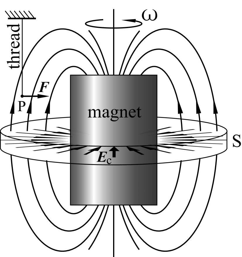
Figure 1: Electric force on the testing charge. When the magnet rotates, does the electric force F appear? The M hypothesis and the Maxwell’s equation will give the opposite answers to this question.

In the light of the inference of the M hypothesis, when the magnet in Fig. 1 rotates, the magnetic field lines rotating with the magnet together will apply an electric force F on the testing charge P suspended in the magnetic field. However, as we know, the electric field E anywhere can be described as

$$\emph{{E}}=\emph{{E}}_{c}+\emph{{E}}_{i},$$ (3)

where $\emph{{E}}_{c}$ is the electric field energized by the charges and $\emph{{E}}_{i}$ is the vortex electric field induced by the change of magnetic field. The following equations can be derived from Maxwell’s equations:

$$\left\{\begin{array}[]{l}\nabla\cdot\textbf{\emph{E}}_{c}=\rho/\varepsilon_{0}\;\left(\textup{or}\;\oint_{\,S}\textbf{\emph{E}}_{c}\cdot\mathrm{d}\textbf{\emph{S}}=Q/\varepsilon_{0}\right),\\ \nabla\times\textbf{\emph{E}}_{c}=0,\end{array}\right.$$ (4)

and

$$\left\{\begin{array}[]{l}\nabla\times\emph{{E}}_{i}=-\,\partial\emph{{B}}/\partial t,\\ \nabla\cdot\textbf{\emph{E}}_{i}=0.\end{array}\right.$$ (5)

If there is an electric field $\emph{{E}}_{c}$ when a magnet rotates, it is certain that this electric field will be symmetrically distributed around the axis of the magnet (shown in Fig 1). As long as the quantity of electric charge in the closed surface S is zero, that is, Q=0, Equation (4) implies the electric field $\emph{{E}}_{c}$ is zero. Therefore, provided the magnet has no charges, no matter whether it rotates or not, the electric field $\emph{{E}}_{c}$ will always be zero. On the other hand, whether the magnet rotates or not, B is always a constant everywhere, while according to Equation (5), the curl of the vortex electric field $\emph{{E}}_{i}$ is zero and clearly $\emph{{E}}_{i}$ also vanishes. In other words, according to Maxwell’s equations, no matter whether the magnet rotates or not, there is no electric field E in the outside space around the magnet and it is impossible to apply an electric field force F on the charge P. However, the M hypothesis infers that the charge P can be acted upon by the electric field force, thus contradicting Maxwell’s equations. Therefore, we suggest the M hypothesis is flawed and that the N hypothesis should be applied to the study of astrophysics.

Unfortunately, the M hypothesis has had an important influence on the pulsar theory. Current consensus in the scientific community appears to be that general physicists prefer the N hypothesis, whereas almost all astrophysicists prefer the M hypothesis. We therefore believe it is worthwhile to discuss the nature of the magnetic field in more detail, to highlight the shortcomings of the M hypothesis. For this reason, we designed a set of cartoons depicting the moving characteristics of the magnetic field, which are available for viewing at http://www.pulsar2.com/English/fieldfilm1.htm.

The corotation model proposed in GJ69 is based on the M hypothesis, which contradicts Maxwell’s equation. Therefore, it cannot be valid.

2.3 Effect of Frozen-in Field Lines

The point of view of GJ69, based on the so-called effect of frozen-in field lines deduced from magnetohydrodynamics, is that the magnetosphere particles cannot travel perpendicularly to the field lines. Here we will show that this concept is untenable.

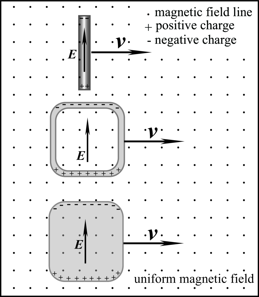
Figure 2: The frozen-in effect. Whether the ideal conductive fluid can be frozen with the magnetic field lines together or not when moving in the uniform magnetic field, the magnetohydrodynamics holds the opposite opinion from the general physics. The mistake of the magnetohydrodynamics is that it irrelevantly omitted the existence of the polarized charges and electric field.

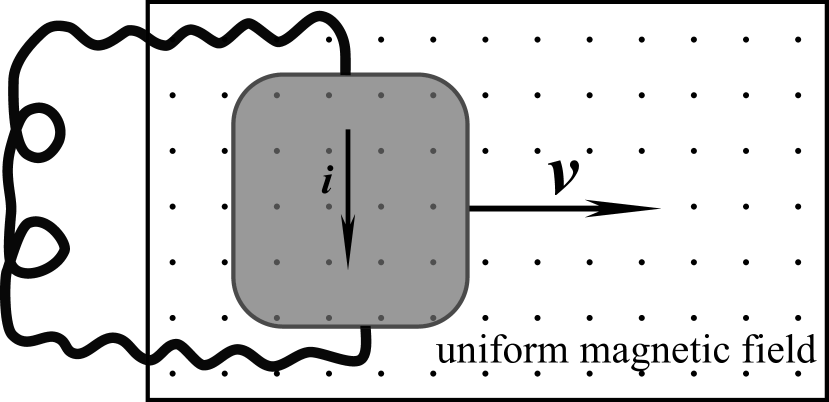
Figure 3: The influence of boundary condition on the frozen-in effect. Only when the polarized charges of the boundary can continuously flow away and the current i forms, the frozen-in effect will occur.

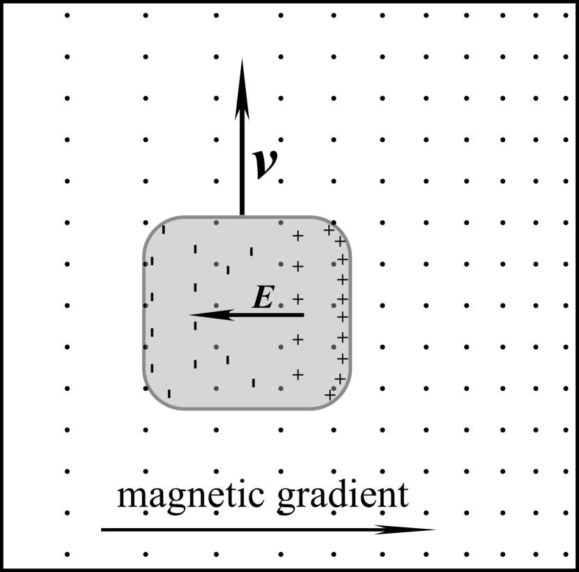
Figure 4: The second non-frozen situation. Even if the conductive fluid moves in the nonuniform magnetic field, as long as it moves along an isomagnetic surface, the frozen-in effect will not occur.

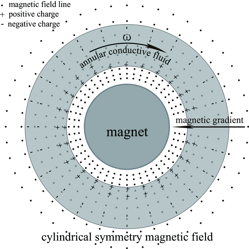
Figure 5: The third non-frozen situation. In the cylindrically symmetrical magnetic field, the rotation of the conductive fluid around the magnetic axle does not lead to the generation of the magnetic frozen phenomenon either, because this induced electric field has zero curl, which is just the same situation in the vicinity of pulsar’s equator.

According to general physics, a wire, annular wire or plate made up of conducting material (Fig. 2), when moving with constant velocity in a uniform magnetic field and cutting the magnetic field lines, can neither produce electric current, nor receive any resistance from the magnetic field, so that the conductors cannot be frozen together with the magnetic field. This conclusion is independent of both the kind and the conductivity of materials, even if a conductive fluid such as mercury or plasma is used to make the objects shown in Fig.2, so the frozen field phenomenon cannot exist. However, the magnetohydrodynamical theory states that an ideal conductive fluid is frozen in the magnetic field and that it cannot travel across the field lines. Thus, there is a contradiction.

We have found that in all studies of the frozen-in effect, the polarization charges and the electric field E shown in Fig. 2 were irrelevantly disregarded. It is the electric field E that thaws the frozen phenomenon and can be simply calculated using the drift theory of charged particles, whereby the drift velocity driven by the electric field E is equal to the advection velocity of the fluid v, that is to say $\emph{{v}}\!_{shift}\equiv\emph{{v}}$. The direction of the drift velocity $\emph{{v}}\!_{shift}$ is always perpendicular to both the electric field and the magnetic field. Therefore, the conductive fluid can cross a uniform magnetic field without any resistance and cannot be frozen together with the magnetic field lines.

If a wire is connected to the two ends of the conductor and the charges are allowed to flow out, as shown in Fig. 3, the current i and the frozen-in field effect will appear and the magnetic field will exert a resistance on the conductor. Consequently, the existence of the frozen phenomenon in a uniform magnetic field is a function of the boundary conditions of the fluid. If the charges can continuously flow, with current i, the frozen phenomenon can be manifested. Otherwise, there is no frozen phenomenon.

An ideal conductive fluid can cross not only a uniform magnetic field, but also a non-uniform field, still free from any resistance, providing the fluid moves along an isomagnetic surface of the magnetic field as shown in Fig. 4. This conclusion can be obtained from the frozen-in field equation:

$$\frac{\partial\mathbf{\emph{{B}}}}{\partial{t}}=\nabla\times(\emph{{v}}\times\emph{{B}}),$$ (6)

where v is the velocity of the conductive fluid elements moving through the magnetic field, and v$\times$B is the induced electric field.

As we know, the essential condition under which a force can exist between the conductive fluid and magnetic field is that of the existence of an eddy current inside the conductive fluid, and the essential condition for the existence of an eddy current appearing is an eddy induced electric field. When both sides of Equation (6) are equal to zero, the induced electric field inside the conductive fluid is an irrotational field. In this case, there is neither an eddy electric field nor an eddy current in the conductive fluid. Sequentially, there is no magnetic force acting on the conductive fluid when it passes through the magnetic field with velocity v. This case is a special solution of the frozen-in field equation (6).

The frozen-in field equation (6) can be expanded as:

$$\frac{\partial\mathbf{\emph{{B}}}}{\partial{t}}=\textbf{\emph{v}}(\nabla\cdot\emph{{B}})-\textbf{\emph{B}}(\nabla\cdot\emph{{v}})-(\textbf{\emph{v}}\cdot\nabla)\emph{{B}}+(\textbf{\emph{B}}\cdot\nabla)\emph{{v}}.$$ (7)

The first term on the right-hand side includes the divergence of the magnetic field $\nabla\cdot\emph{{B}}$, therefore, this term is always zero.

The factor $\nabla\cdot\emph{{v}}$ in the second term is the divergence of the velocity field. When the fluid moves without expansion or compression (i.e., the bulk has not change), this term is also zero.

When the path of each conductive fluid element follows an isomagnetic surface (i.e., constant B), the third term $(\textbf{\emph{v}}\cdot\nabla)\emph{{B}}$ is also equal to zero.

If all of the fluid elements threaded by a magnetic field line have the same velocity, without differential movement, the fourth term $(\textbf{\emph{B}}\cdot\nabla)\emph{{v}}$ is also zero. If the shapes of magnetic field lines have not change and this term is not equal to zero, the shape of the fluid will change.

Therefore, providing the shape and the size of the conductive fluid remain the same, all of the situations shown in Fig. 2, Fig. 4 and Fig. 5 correspond to a special solution where all four terms are zero in the right-hand side of equation (7). In these cases the induced electric field inside the conductive fluid are irrotational, and the frozen-in phenomenon is not manifested. Because the case illustrated in Fig. 5 is equivalent to that in the vicinity of a pulsar’s equator, the viewpoint that the plasma of a pulsar cannot cross the magnetic field lines is inaccurate.

Another description of the frozen-in field equation is

$$\frac{d\Phi}{dt}=0.$$ (8)

From this equation, one can see that the essence of the frozen-in field theorem is the conservation of magnetic flux inside the fluid. This conservation principle does not imply that the conductive fluid cannot pass through magnetic field lines, only that the magnetic field lines entering a given fluid element are equal in number to those leaving the element at all times.

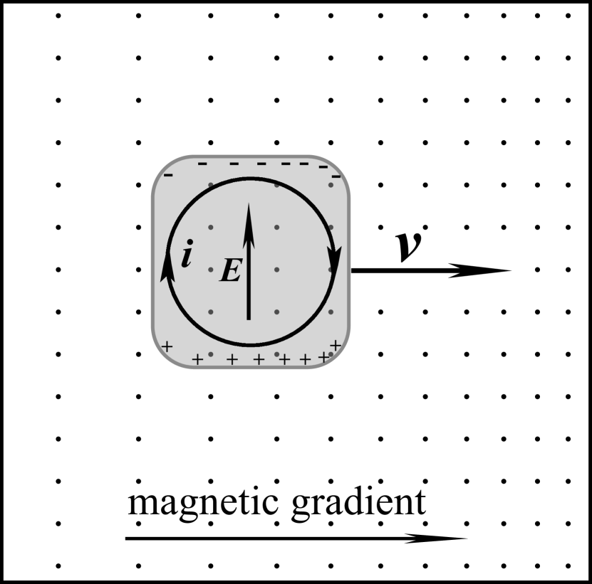
Figure 6: A frozen-in situation. The movement of the conductive fluid, if the velocity has a component in the direction of the magnetic gradient, will lead to the emergence of the frozen-in effect.

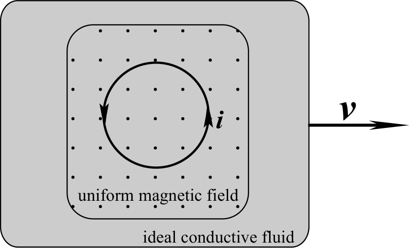
Figure 7: Another frozen-in situation. If the size of the magnetic field is smaller than the size of the conductive fluid, even if the magnetic field is uniform, the frozen-in effect will also occur, because the magnetic field has a high gradient near its boundary.

On the condition that the shape and the size of the conductive fluid do not change, two frozen examples are respectively shown in Fig. 6 and Fig. 7. In general, if the magnetic field intensity in the direction of travel of the conductive fluid changes, the conductive fluid will be acted upon by the frozen resistance.

Further, when an individual charged particle crosses a magnetic field the Lorentz force will compel it to gyrate around the magnetic field lines. However, within the conductive fluid, the appearances of polarization charges and a polarization electric field create a very different situation. Under some special conditions such as those illustrated in Figs. 2, 4 and 5, the polarized electric field can counteract the Lorentz force and allow the conductive fluid to cross the magnetic field without any resistance.

3 Magnetohydrodynamic experiments

To illustrate the above analysis, we conducted a series of magnetohydrodynamic experiments.

The main materials used in our experiments were liquid mercury and solid magnets. The mercury simulated the plasma, while the magnet simulated the pulsar. For the sake of simplicity and clarity, our experiments were recorded as videos which are available at YouTube. Briefly, the mercury is placed in a cylindrical trough surrounding a rotating platform with a receptacle for the solid magnet.

The experiments were divided into two subgroups. The first consisted of three pairs of experiments whose purpose was to ascertain the conditions under which the magnet can drive rotation in the surrounding mercury. In each experiment our basis for comparison was an aligned rotator : a cylindrically symmetric magnet whose magnetic axis is the same as the axis of rotation. The three experiment pairs were as follows:

1. Drive Experiment A shows the contrast between the aligned rotator and a rotator whose magnetic axis is orthogonal to the axis of rotation. The URL is

   http://www.youtube.com/watch?v=YCc4ybfKiY0.

2. Drive Experiment B shows the contrast between the aligned rotator and a magnet whose magnetic axis is parallel to but displaced from the axis of rotation. This video can be found at

   http://www.youtube.com/watch?v=ZiVNxVAqUKc.

3. Drive Experiment C shows the contrast between the aligned rotator and a magnet which is not cylindrically symmetric. The video is at URL

   http://www.youtube.com/watch?v=SBAzUBzc2xM.

The first subgroup of experiments demonstrates that a cylindrically symmetric magnetic fieldcannot drive the mercury when its magnetic axis is the same as the axis of rotation. When the magnetic axis is unaligned with the spin axis or the distribution of the magnetic field is not cylindrically symmetric, however, the mercury can be driven.

In the second subgroup of experiments, we ascertain the conditions under which rotating mercury can be slowed down by a stationary magnet. To do so, we spun the mercury trough rather than the central magnet until the mercury’s revolution reached a steady state. In each experiment our basis of comparison was again an aligned magnet : a cylindrically symmetric magnet whose magnetic axis was the same as the axis of rotating mercury. With the aligned magnet, the mercury eventually revolved at the same rate as the trough. In the other three cases, braking forces limited the mercury to a slower rate. We used the same magnets in every pair of experiments seen in Braking Experiments A, B and C.

1. Braking Experiment A shows the contrast between the aligned magnet and the orthogonal magnet, and can be viewed at

   http://www.youtube.com/watch?v=C7DxRoVdtxw.

2. Braking Experiment B shows the contrast between the aligned magnet and the off-axis magnet, and can be viewed at

   http://www.youtube.com/watch?v=p9UzfT6UHcE.

3. Braking Experiment C shows the contrast between the aligned magnet and the magnet which is cylindrically asymmetric, and can be viewed at

   http://www.youtube.com/watch?v=Eq0B5XR_o8U.

These experiments demonstrate that a coaxial, cylindrically symmetric magnetic field has no braking effect on the mercury. In other words, under some special conditions the mercury can cross the magnetic field lines without experiencing a braking force. The magnet can exert a braking effect on the mercury only when its magnetic axis is unaligned with the axis of mercury rotation or when the magnetic field is not cylindrically symmetrical.

4 Discussion

The experimental results reveal two phenomena worthy of special attention:

1. A rotating magnet cannot drive the stationary mercury when the axes of rotation of the mercury and the magnet are identical. This result is apparent based on the N hypothesis, because the stationary magnetic field lines are unable to induce rotation in the mercury.

2. A stationary magnet cannot slow down revolving mercury when the axis of rotation is identical to the magnetic axis. This result is apparent based on the analytical results in Section 2.3 and Fig. 5.

In summary, no exchange of angular momentum will occur between the magnet and the mercury under conditions where the magnetic field and the mercury share cylindrical symmetry. The degrees of axial alignment and symmetry thus control the exchange of the angular momentum. Of course, a change of magnetic flux through each fluid element is a necessary condition for the exchange of angular momentum.

The plasma surrounding a pulsar covers the entire spherical surface. In our experiments, the mercury circulates within a region near the equatorial plane. Therefore, the results of our study are only directly comparable to the behavior of plasma near the equatorial plane.

The above discussion refers only to aligned pulsars. Pulsars with unaligned magnetic fields are more complicated. As shown in
http://www.pulsar2.com/English/fieldfilm7.htm, while the magnetic axis of an oblique rotator swings around, the magnetic field lines do not rotate around the magnetic axis. When the magnetic dip angle is small, the magnetic field lines near the equatorial plane can be considered approximately stationary. Thus, our results are still noteworthy.

Results presented by both GJ69 and the present paper are based on the theory of classical mechanics without considering relativistic effects in the plasma. Even if it is necessary to consider these effects, we can make relativistic corrections to the classical mechanics, but the laws of classical mechanics can never be violated. However, ideas proposed by GJ69 contradict the laws of classical mechanics.

5 Conclusions

The following conclusions can be drawn from our experiments and analysis:

1. Three mistakes were made by GJ69: first, the relative velocity is irrelevantly replaced by the corotation velocity; second, their theory is based on the M hypothesis which is contradictory to Maxwell’s equations; and third, their theory neglected a special solution of the frozen-in field equation which is of particular importance for pulsar research.

2. The magnetic field near the equatorial plane of an aligned pulsar is steady, so it can neither drive nor brake the plasma. Thus, the viewpoint that magnetosphere particles can only move along magnetic field lines is wrong and the corotation model is flawed.

3. The corotation model should be abandoned and the models of pulsar electrodynamics should be reformulated under new assumptions.

References

- Goldreich & Julian (1969) Goldreich, P. & Julian, W. H., 1969, ApJ, 157, 869
- Lyne & Graham-Smith (2006) Lyne, A. & Graham-Smith, F., 2006, Pulsar Astronomy, p22(third ed.; Cambridge University Press)