Formal-language-theoretic Optimal Path Planning
For Accommodation of Amortized Uncertainties and Dynamic Effects

Abstract

We report a globally-optimal approach to robotic path planning under uncertainty, based on the theory of quantitative measures of formal languages. A significant generalization to the language-measure-theoretic path planning algorithm $\boldsymbol{\nu^{\star}}$ is presented that explicitly accounts for average dynamic uncertainties and estimation errors in plan execution. The notion of the navigation automaton is generalized to include probabilistic uncontrollable transitions, which account for uncertainties by modeling and planning for probabilistic deviations from the computed policy in the course of execution. The planning problem is solved by casting it in the form of a performance maximization problem for probabilistic finite state automata. In essence we solve the following optimization problem: Compute the navigation policy which maximizes the probability of reaching the goal, while simultaneously minimizing the probability of hitting an obstacle. Key novelties of the proposed approach include the modeling of uncertainties using the concept of uncontrollable transitions, and the solution of the ensuing optimization problem using a highly efficient search-free combinatorial approach to maximize quantitative measures of probabilistic regular languages. Applicability of the algorithm in various models of robot navigation has been shown with experimental validation on a two-wheeled mobile robotic platform (SEGWAY RMP 200) in a laboratory environment.

1 Introduction & Motivation

The objective of this paper is to report a globally-optimal approach to path planning under uncertainty, based on the theory of quantitative measures of formal languages. The field of trajectory and motion planning is enormous, with applications in such diverse areas as industrial robots, mobile robot navigation, spacecraft reentry, video games and even drug design. Many of the basic concepts are presented in  [Lat91] and in recent comprehensive surveys [Lav06]. In the context of planning for mobile robots and manipulators much of the literature on path and motion planning is concerned with finding collision-free trajectories [KK92]. A great deal of the complexity in these problems arises from the topology of the robot’s configuration space, called the $\mathcal{C}$-Space. Various analytical techniques, such as wavefront expansion [BK02] and cellular decomposition, have been reported in recent literature [Lp87], which partition the $\mathcal{C}$-Space into a finite number of regions with the objective of reducing the motion planning problem as identification of a sequence of neighboring cells between the initial and final (i.e., goal) regions. Graph-theoretic search-based techniques have been used somewhat successfully in many wheeled ground robot path planning problems and have been used for some UAV planning problems, typically radar evasion [AniHamHu03]. These approaches typically suffer from complexity issues arising from expensive searches, particularly in complicated configuration spaces. To circumvent the complexity associated with graph-based planning, sampling based planning methods [BLL90] such as probabilistic roadmaps have been proposed. However, sampling based approaches are only probabilistically complete (i.e. if a feasible solution exists it will be found, given enough time) but there is no guarantee of finding a solution within a specified time, and more often than not, global route optimality is not guaranteed. Distinct from these general approaches, there exist reported techniques that explicitly make use of physical aspects of specific problems for planning $e.g.$ use of vertical wind component for generating optimal trajectories for UAVs [Lan08], feasible collision-free trajectory generation for cable driven platforms [LOZRC09], and the recently reported approach employing angular processing [Ort09].

1.1 Potential Field-based Planning Methodology

Among reported deterministic approaches, methods based on artificial potential fields have been extensively investigated, often referred to cumulatively as potential field methods (PFM). The idea of imaginary forces acting on a robot were suggested by several authors inclding [AH83] and [Kh85]. In these approaches obstacles exert repulsive forces onto the robot, while the target applies an attractive force to the robot. The resultant of all forces determines the subsequent direction and speed of travel. One of the reasons for the popularity of this method is its simplicity and elegance. Simple PFMs can be implemented quickly and initially provide acceptable results without requiring many refinements. [Kr84] has suggested a generalized potential field method that combines global and local path planning. Potential field based techniques have been also successfully employed in multi-robot co-operative planning scenarios [KGZ07, SHK08], where other techniques prove to be inefficient and impractical.

While the potential field principle is particularly attractive because of its elegance and simplicity, substantial shortcomings have been identified that are inherent to this principle. The interested reader is referred to [BK91-1] for a systematic criticism of PFM-based planning, where the authors cite the underlying differential equation based analysis as the source of the problems, and the fact that it combines the robot and the environment into one unified system. Key problems inherent to PFMs, independent of the particular implementation, are:

1. Trap situations due to local minima: Perhaps the best-known problem with PFMs are possible trap-situations [AH83, Ti90], which occur when when the robot runs into a dead end, due to the existence of a local extrema in the potential field. Trap-situations can be remedied with heuristic recovery rules, which are likely to result in non-optimal paths.

2. No passage between closely spaced obstacles: A severe problem with PFMs occurs when the robot attempts to travel through narrow corridors thereby experiencing repulsive forces simultaneously from opposite sides, leading to wavy trajectories, no passage etc.

3. Oscillations in the presence of obstacles: Presence of high obstacle clutter often leads to unstable motion, due to the complexity of the resultant potential.

4. Effect of past obstacles: Even after the robot has already passed an obstacle, the latter keeps affecting the robot motion for a significant period of time (until the repulsive potential dies down).

These disadvantages become more apparent when the PFM-based methods are implemented in high-speed real-time systems; simulations and slow speed experiments often conceal the issues; probably contributing to the widespread popularity of potential planners.

1.2 The $\boldsymbol{\nu^{\star}}$ Planning Algorithm

Recently, the authors reported a novel path planning algorithm $\boldsymbol{\nu^{\star}}$ [CMR08], that models the navigation problem in the framework of Probabilistic Finite State Automata (PFSA) and computes optimal plans via optimization of the PFSA from a strictly control-theoretic viewpoint. $\boldsymbol{\nu^{\star}}$ uses cellular decomposition of the workspace, and assumes that the blocked grid locations can be easily estimated, upon which the planner computes an optimal navigation gradient that is used to obtain the routes. This navigation gradient is computed by optimizing the quantitative measure of the probabilistic formal language generated by the associated navigation automaton. The key advantages can be enumerated as:

1. $\boldsymbol{\nu^{\star}}$ is fundamentally distinct from a search: The search problem is replaced by a sequential solution of sparse linear systems. On completion of cellular decomposition, $\boldsymbol{\nu^{\star}}$ optimizes the resultant PFSA via a iterative sequence of combinatorial operations which elementwise maximizes the language measure vector [CR06][CR07]. Note that although $\boldsymbol{\nu^{\star}}$ involves probabilistic reasoning, the final waypoint sequence obtained is deterministic.

2. Computational efficiency: The intensive step in $\boldsymbol{\nu^{\star}}$ is a special sparse matrix inversion to compute the language measure. The time complexity of each iteration step can be shown to be linear in problem size implying significant numerical advantage over search-based methods for high-dimensional problems.

3. Global monotonicity: The solution iterations are globally monotonic, $i.e$, each iteration yields a better approximation to the final optimal solution. The final waypoint sequence is generated essentially by following the measure gradient which has a unique maxima at the goal.

4. Global Optimality: It can be shown that trap-situations are a mathematical impossibility for $\boldsymbol{\nu^{\star}}$.

The optimal navigation gradient produced by $\boldsymbol{\nu^{\star}}$ is reminiscent of potential field methods [BLL90]. However, $\boldsymbol{\nu^{\star}}$ automatically generates, and optimizes this gradient; no ad-hoc potential function is necessary.

1.3 Focus of Current Work & Key Contributions

The key focus of this paper is extension of the $\boldsymbol{\nu^{\star}}$ planning algorithm to optimally handle execution uncertainties. It is well recognized by domain experts that merely coming up with a navigation plan is not sufficient; the computed plan must be executed in the real world by the mobile robot, which often cannot be done exactly and precisely due to measurement noise in the exteroceptive sensors, imperfect actuations, and external disturbances. The idea of planning under uncertainties is not particularly new, and good surveys of reported methodologies exist [JTCL05]. In chronological order, the main family of reported approaches can be enumerated as follows:

• Pre-image Back-chaining [LP84, ll92, fm98] where the plan is synthesized by computing a set of configurations from which the robot can possibly reach the goal, and then propgating this preimage recursively backward or back-chaining, a problem solving approach originally proposed in [Ni80].

• Approach based on sensory uncertainty fields (SUF) [tl92, tk96, vt98, rt99] computed over the collision-free subset of the robot’s configuration space, which reflects expected uncertainty (distribution of possible errors) in the sensed configuration that would be computed by matching the sensory data against a known environment model ($e.g.$ landmark locations). A planner then makes use of the computed SUF to generate paths that minimize expected errors.

• Sensor-based planning approaches [as94, bsa95, kbsc97], which consider explicit uncertainty models of various motion primitives to compute a feasible robust plan composed of sensor-based motion commands in polygonal environments, with significant emphasis on wall-following schemes.

• Information space based approach using the Bellman principle of stochastic dynamic programming [BF95], which introduced key concepts such as setting up the problem in a probabilistic framework, and demanding that the optimal plan maximize the probability of reaching the goal. However, the main drawback was the exponential dependence on the dimension of the computed information space.

• The set-membership approach [PS95] which performs a local search, trying to deform a path into one that respects uncertainty constraints imposed by arbitrarily shaped uncertainty sets. Each hard constraint is turned into a soft penalty function, and the gradient descent algorithm is employed, hoping convergence to an admissible solution.

• Probabilistic approaches based on disjunctive linear programming [blw06, b06], with emphasis on UAV applications. The key limitation is the inability to take into account exteroceptive sensors, and also the assumption that dead-reckoning is independent of the path executed. Later extensions of this approach use particle representations of the distributions, implying wider applicability.

• Adaptation of search strategies in extended spaces [lf00, LG03, gs05, gs07], which consider the classical search problem in configuration spaces augmented with uncertainty information.

• Approach based on Stochastic Motion Roadmaps (SRM) [ASG07], which combines sampling-based roadmap representation of the configuration space, with the theory of Markov Decision Processes, to yield models that can be subsequently optimized via value-iteration based infinite horizon dynamic programming, leading to plans that maximize the probability of reaching the goal.

The current work adds a new member to the family of existing approaches to address globally optimal path planning under uncertainties. The key novelty of this paper is the association of uncertainty with the notion of uncontrollability in a controlled system. The navigation automaton introduced in  [CMR08] is augmented with uncontrollable transitions which essentially captures the possibility that the agent may execute actuation sequences (or motion primitives) that are not coincident with the planned moves. The planning objective is simple: Maximize the probability of reaching the goal, while simultaneously minimizing the probability of hitting any obstacle. Note that, in this respect, we are essentially solving the exact same problem investigated by  [ASG07]. However our solution approach is very different. Instead of using value iteration based dynamic programming, we use the theory of language-measure-theoretic optimization of probabilistic finite state automata [CR07]. Unlike the SRM approach, the proposed algorithm does not require the use of local auxiliary planners, and also needs to make no assumptions on the structure of the configuration space to guarantee iterative convergence. The use of arbitrary penalties for reducing the weight on longer paths is also unnecessary, which makes the proposed $\boldsymbol{\nu^{\star}}$ under uncertainties completely free from heuristics. We show that all the key advantages that $\boldsymbol{\nu^{\star}}$ has over the state-of-art carries over to this more general case; namely that of significantly better computational efficiency, simplicity of implementation, and achieving global optimality via monotonic sequence of search-free combinatorial iterative improvements, with guaranteed polynomial convergence. The proposed approach thus solves the inherently non-convex optimization [SS08] by mapping the physical specification to an optimal control problem for probabilistic finite state machines (the navigation automata), which admits efficient combinatorial solutions via the language-measure-theoretic approach. The source of many uncertainties, namely modeling uncertainty, disturbances, and uncertain localization, is averaged over (or amortized) for adequate representation in the automaton framework. This may be viewed as a source of approximation in the proposed approach; however we show in simulation and in actual experimentation that the amortization is indeed a good approach to reduce planning complexity and results in highly robust planning decisions. Thus the modified language-measure-theoretic approach presented in this paper, potentially lays the framework for seamless integration of data-driven and physics-based models with the high-level decision processes; this is a crucial advantage, and goes to address a key issue in autonomous robotics, $e.g.$, in a path-planning scenario with mobile robots, the optimal path may be very different for different speeds, platform capabilities and mission specifications. Previously reported approaches to handle these effects using exact differential models of platform dynamics results in overtly complex solutions that do not respond well to modeling uncertainties, and more importantly to possibly non-stationary environmental dynamics and evolving mission contexts. Thus the measure-theoretic approach enables the development of true Cyber-Physical algorithms for control of autonomous systems; algorithms that operate in the logical domain while optimally integrating, and responding to, physical information in the planning process.

The rest of the paper is organized in seven sections. Section 2 briefly explains the language-theoretic models considered in this paper, reviews the language-measure-theoretic optimal control of probabilistic finite state machines and presents the necessary details of the reported $\boldsymbol{\nu^{\star}}$ algorithm. Section 3 presents the modifications to the navigation model to incorporate the effects of dynamic uncertainties within the framework of probabilistic automata. Section 4 presents the pertinent theoretical results and establishes the main planning algorithm. Section 5 develops a formulation to identify the key amortized uncertainty parameters of the PFSA-based navigation model from an observed dynamical response of a given platform. The proposed algorithm is summarized with pertinent comments in Section 6. The theoretical development is verified in high-fidelity simulations on different navigation models and validated in experimental runs on the SEGWAY RMP 200 in section LABEL:secvv. The paper is summarized and concluded in Section LABEL:secsummary with recommendations for future work.

2 Preliminaries: Language Measure-theoretic Optimization Of Probabilistic Automata

This section summarizes the signed real measure of regular languages; the details are reported in [R05]. Let $G_{i}\equiv\langle Q,\Sigma,\delta,q_{i},Q_{m}\rangle$ be a trim (i.e., accessible and co-accessible) finite-state automaton model that represents the discrete-event dynamics of a physical plant, where $Q=\{q_{k}:k\in\mathcal{I}_{Q}\}$ is the set of states and $\mathcal{I}_{Q}\equiv\{1,2,\cdots,n\}$ is the index set of states; the automaton starts with the initial state $q_{i}$; the alphabet of events is $\Sigma=\{\sigma_{k}:k\in\mathcal{I}_{\Sigma}\}$, having $\Sigma\bigcap\mathcal{I}_{Q}=\emptyset$ and $\mathcal{I}_{\Sigma}\equiv\{1,2,\cdots,\ell\}$ is the index set of events; $\delta:Q\times\Sigma\rightarrow Q$ is the (possibly partial) function of state transitions; and $Q_{m}\equiv\{q_{m_{1}},q_{m_{2}},\cdots,q_{m_{l}}\}\subseteq Q$ is the set of marked (i.e., accepted) states with $q_{m_{k}}=q_{j}$ for some $j\in\mathcal{I}_{Q}$. Let $\Sigma^{*}$ be the Kleene closure of $\Sigma$, i.e., the set of all finite-length strings made of the events belonging to $\Sigma$ as well as the empty string $\epsilon$ that is viewed as the identity of the monoid $\Sigma^{*}$ under the operation of string concatenation, i.e., $\epsilon s=s=s\epsilon$. The state transition map $\delta$ is recursively extended to its reflexive and transitive closure $\delta:Q\times\Sigma^{*}\rightarrow Q$ by defining $\forall q_{j}\in Q,\ \delta(q_{j},\epsilon)=q_{j}$ and $\forall q_{j}\in Q,\sigma\in\Sigma,s\in\Sigma^{\star},\ \delta(q_{i},\sigma s)=\delta(\delta(q_{i},\sigma),s)$

Definition 1.

The language $L(q_{i})$ generated by a DFSA $G$ initialized at the state $q_{i}\in Q$ is defined as: $L(q_{i})=\{s\in\Sigma^{*}\ |\ \delta^{*}(q_{i},s)\in Q\}$ The language $L_{m}(q_{i})$ marked by the DFSA $G$ initialized at the state $q_{i}\in Q$ is defined as: $L_{m}(q_{i})=\{s\in\Sigma^{*}\ |\ \delta^{*}(q_{i},s)\in Q_{m}\}$

Definition 2.

For every $q_{j}\in Q$, let $L(q_{i},q_{j})$ denote the set of all strings that, starting from the state $q_{i}$, terminate at the state $q_{j}$, i.e., $L_{i,j}=\{s\in\Sigma^{*}\ |\ \delta^{*}(q_{i},s)=q_{j}\in Q\}$

The formal language measure is first defined for terminating plants [G92, G92-2] with sub-stochastic event generation probabilities $i.e.$ the event generation probabilities at each state summing to strictly less than unity.

Definition 3.

The event generation probabilities are specified by the function $\tilde{\pi}:\Sigma^{\star}\times\,Q\to[0,\,1]$ such that $\forall q_{j}\in Q,\forall\sigma_{k}\in\Sigma,\forall s\in\Sigma^{\star},$

1. $\tilde{\pi}({\sigma_{k}},q_{j})\triangleq\tilde{\pi}_{jk}\in[0,1)$;  $\sum_{k}\tilde{\pi}_{jk}=1-\theta,\ \mathrm{with}\ \theta\in(0,1)$;

2. $\tilde{\pi}(\sigma,q_{j})=0$ if $\delta(q_{j},\sigma)$ is undefined; $\ \tilde{\pi}(\epsilon,q_{j})=1$;

3. $\tilde{\pi}({\sigma_{k}s},q_{j})=\tilde{\pi}({\sigma_{k}},q_{j})\ \tilde{\pi}(s,\delta(q_{j},\sigma_{k}))$.

The $n\times\ell$ event cost matrix is defined as: $\mathbf{\widetilde{\Pi}}|_{ij}=\tilde{\pi}(q_{i},\sigma_{j})$

Definition 4.

The state transition probability $\pi:Q\times Q\rightarrow[0,1)$, of the DFSA $G_{i}$ is defined as follows: $\forall q_{i},q_{j}\in Q,\pi_{ij}=\displaystyle\sum_{\sigma\in\Sigma\ \mathrm{s.t.}\ \delta(q_{i},\sigma)=q_{j}}\tilde{\pi}(\sigma,q_{i})$ The $n\times n$ state transition probability matrix is defined as $\mathbf{\Pi}|_{jk}=\pi(q_{i},q_{j})$

The set $Q_{m}$ of marked states is partitioned into $Q_{m}^{+}$ and $Q_{m}^{-}$, i.e., $Q_{m}=Q_{m}^{+}\cup Q_{m}^{-}$ and $Q_{m}^{+}\cap Q_{m}^{-}=\emptyset$, where $Q_{m}^{+}$ contains all good marked states that we desire to reach, and $Q_{m}^{-}$ contains all bad marked states that we want to avoid, although it may not always be possible to completely avoid the bad states while attempting to reach the good states. To characterize this, each marked state is assigned a real value based on the designer’s perception of its impact on the system performance.

Definition 5.

The characteristic function $\chi:Q\rightarrow[-1,1]$ that assigns a signed real weight to state-based sublanguages $L(q_{i},q)$ is defined as:

$$\forall q\in Q,\quad\chi(q)\in\left\{\begin{array}[]{cc}[-1,0),&q\in Q_{m}^{-}\\ \{0\},&q\notin Q_{m}\\ \rm{(0,1]},&\it{q}\in Q_{m}^{+}\end{array}\right.$$ (1)

The state weighting vector, denoted by $\boldsymbol{\chi}=[\chi_{1}\ \chi_{2}\ \cdots\ \chi_{n}]^{T}$, where $\chi_{j}\equiv\chi(q_{j})$ $\forall j\in\mathcal{I}_{Q}$, is called the $\boldsymbol{\chi}$-vector. The $j$-th element $\chi_{j}$ of $\boldsymbol{\chi}$-vector is the weight assigned to the corresponding terminal state $q_{j}$.

In general, the marked language $L_{m}(q_{i})$ consists of both good and bad event strings that, starting from the initial state $q_{i}$, lead to $Q_{m}^{+}$ and $Q_{m}^{-}$ respectively. Any event string belonging to the language $L^{0}=L(q_{i})-L_{m}(q_{i})$ leads to one of the non-marked states belonging to $Q-Q_{m}$ and $L^{0}$ does not contain any one of the good or bad strings. Based on the equivalence classes defined in the Myhill-Nerode Theorem, the regular languages $L(q_{i})$ and $L_{m}(q_{i})$ can be expressed as: $L(q_{i})=\bigcup_{q_{k}\in Q}L_{i,k}$ and $L_{m}(q_{i})=\bigcup_{q_{k}\in Q_{m}}L_{i,k}=L_{m}^{+}\cup L_{m}^{-}$ where the sublanguage $L_{i,k}\subseteq G_{i}$ having the initial state $q_{i}$ is uniquely labelled by the terminal state $q_{k},k\in\mathcal{I}_{Q}$ and $L_{i,j}\cap L_{i,k}=\emptyset$ $\forall j\neq k$; and $L_{m}^{+}\equiv\bigcup_{q_{k}\in Q_{m}^{+}}L_{i,k}$ and $L_{m}^{-}\equiv\bigcup_{q_{k}\in Q_{m}^{-}}L_{i,k}$ are good and bad sublanguages of $L_{m}(q_{i})$, respectively. Then, $L^{0}=\bigcup_{q_{k}\notin Q_{m}}L_{i,k}$ and $L(q_{i})=L^{0}\cup L_{m}^{+}\cup L_{m}^{-}$.

A signed real measure $\mu^{i}:{2^{L(q_{i})}}\rightarrow\mathbb{R}\equiv(-\infty,+\infty)$ is constructed on the $\sigma$-algebra $2^{L(q_{i})}$ for any $i\in\mathcal{I}_{Q}$; interested readers are referred to [R05] for the details of measure-theoretic definitions and results. With the choice of this $\sigma$-algebra, every singleton set made of an event string $s\in L(q_{i})$ is a measurable set. By Hahn Decomposition Theorem [R88], each of these measurable sets qualifies itself to have a numerical value based on the above state-based decomposition of $L(q_{i})$ into $L^{0}$(null), $L^{+}$(positive), and $L^{-}$(negative) sublanguages.

Definition 6.

Let $\omega\in L(q_{i},q_{j})\subseteq 2^{L(q_{i})}$. The signed real measure $\mu^{i}$ of every singleton string set $\{\omega\}$ is defined as: $\mu^{i}(\{\omega\})\coloneqq\tilde{\pi}(q_{i},\omega)\chi(q_{j})$. The signed real measure of a sublanguage $L_{i,j}\subseteq L(q_{i})$ is defined as: $\mu_{i,j}\coloneqq\mu^{i}(L(q_{i},q_{j}))=\left(\sum_{\omega\in L(q_{i},q_{j})}\tilde{\pi}(q_{i},\omega)\right)\chi_{j}$

Therefore, the signed real measure of the language of a DFSA $G_{i}$ initialized at $q_{i}\in Q$, is defined as $\mu_{i}\coloneqq\mu^{i}(L(q_{i}))=\sum_{j\in\mathcal{I}_{Q}}\mu^{i}(L_{i,j})$. It is shown in [R05] that the language measure can be expressed as $\mu_{i}=\sum_{j\in\mathcal{I}_{Q}}\mathcal{\pi}_{ij}\mu_{j}+\chi_{i}$. The language measure vector, denoted as $\mu$ = $[\mu_{1}\ \mu_{2}\ \cdots\ \mu_{n}]^{T}$, is called the $\mu$-vector. In vector form, we have $\mbox{\boldmath$\mu$}=\mathbf{\Pi}\mathbf{\mu}+\boldsymbol{\chi}$ whose solution is given by $\mbox{\boldmath$\mu$}=(\mathbf{I}-\mathbf{\Pi})^{-1}\boldsymbol{\chi}$ The inverse exists for terminating plant models [G92] because $\boldsymbol{\Pi}$ is a contraction operator [R05] due to the strict inequality $\sum_{j}\Pi_{ij}<1$. The residual $\theta_{i}=1-\sum_{j}\Pi_{ij}$ is referred to as the termination probability for state $q_{i}\in Q$. We extend the analysis to non-terminating plants with stochastic transition probability matrices ($i.e.$ with $\theta_{i}=0,\ \forall q_{i}\in Q$) by renormalizing the language measure [CR06] with respect to the uniform termination probability of a limiting terminating model as described next.

Let $\widetilde{\Pi}$ and $\Pi$ be the stochastic event generation and transition probability matrices for a non-terminating plant $G_{i}=\langle Q,\Sigma,\delta,q_{i},Q_{m}\rangle$. We consider the terminating plant $G_{i}(\theta)$ with the same DFSA structure $\langle Q,\Sigma,\delta,q_{i},Q_{m}\rangle$ such that the event generation probability matrix is given by $(1-\theta)\widetilde{\Pi}$ with $\theta\in(0,1)$ implying that the state transition probability matrix is $(1-\theta)\Pi$.

Definition 7 (Renormalized Measure).

The renormalized measure $\nu^{i}_{\theta}:2^{L(q_{i}(\theta))}\rightarrow[-1,1]$ for the $\theta$-parametrized terminating plant $G_{i}(\theta)$ is defined as:

$$\forall\omega\in L(q_{i}(\theta)),\ \nu^{i}_{\theta}(\{\omega\})=\theta\mu^{i}(\{\omega\})$$ (2)

The corresponding matrix form is given by $\boldsymbol{\nu_{\theta}}=\theta\ \boldsymbol{\mu}=\theta\ [I-(1-\theta)\Pi]^{-1}\boldsymbol{\chi}\ \mathrm{with}\ \theta\in(0,1)$. We note that the vector representation allows for the following notational simplification $\nu_{\theta}^{i}(L(q_{i}(\theta)))=\boldsymbol{\nu_{\theta}}\big{|}_{i}$ The renormalized measure for the non-terminating plant $G_{i}$ is defined to be $\lim_{\theta\rightarrow o^{+}}\nu_{\theta}^{i}$.

2.1 Event-driven Supervision of PFSA

Plant models considered in this paper are deterministic finite state automata (plant) with well-defined event occurrence probabilities. In other words, the occurrence of events is probabilistic, but the state at which the plant ends up, given a particular event has occurred, is deterministic. Since no emphasis is placed on the initial state and marked states are completely determined by $\chi$, the models can be completely specified by a sextuple as: $G=(Q,\Sigma,\delta,\widetilde{\boldsymbol{\Pi}},\chi,\mathscr{C})$

Definition 8 (Control Philosophy).

If $q_{i}\xrightarrow[\sigma]{}q_{k}$, and the event $\sigma$ is disabled at state $q_{i}$, then the supervisory action is to prevent the plant from making a transition to the state $q_{k}$, by forcing it to stay at the original state $q_{i}$. Thus disabling any transition $\sigma$ at a given state $q$ results in deletion of the original transition and appearance of the self-loop $\delta(q,\sigma)=q$ with the occurrence probability of $\sigma$ from the state $q$ remaining unchanged in the supervised and unsupervised plants. For a given plant, transitions that can be disabled in the sense of Definition 8 are defined to be controllable transitions. The set of controllable transitions in a plant is denoted $\mathscr{C}$. Note controllability is state-based.

2.2 Optimal Supervision Problem: Formulation & Solution

A supervisor disables a subset of the set $\mathscr{C}$ of controllable transitions and hence there is a bijection between the set of all possible supervision policies and the power set $2^{\mathscr{C}}$. That is, there exists $2^{|\mathscr{C}|}$ possible supervisors and each supervisor is uniquely identifiable with a subset of $\mathscr{C}$ and the language measure $\nu$ allows a quantitative comparison of different policies.

Definition 9.

For an unsupervised plant $G=(Q,\Sigma,\delta,\widetilde{\Pi},\chi,\mathscr{C})$, let $G^{{\dagger}}$ and $G^{{\ddagger}}$ be the supervised plants with sets of disabled transitions, $\mathscr{D}^{{\dagger}}\subseteq\mathscr{C}$ and $\mathscr{D}^{{\ddagger}}\subseteq\mathscr{C}$, respectively, whose measures are $\boldsymbol{\nu}^{{\dagger}}$ and $\boldsymbol{\nu}^{{\ddagger}}$. Then, the supervisor that disables $\mathscr{D}^{{\dagger}}$ is defined to be superior to the supervisor that disables $\mathscr{D}^{{\ddagger}}$ if $\boldsymbol{\nu}^{{\dagger}}\geqq_{\textbf{{(Elementwise)}}}\boldsymbol{\nu}^{{\ddagger}}$ and strictly superior if $\boldsymbol{\nu}^{{\dagger}}>_{\textbf{{(Elementwise)}}}\boldsymbol{\nu}^{{\ddagger}}$.

Definition 10 (Optimal Supervision Problem).

Given a (non-terminating) plant $G=(Q,\Sigma,\delta,\widetilde{\Pi},\chi,\mathscr{C})$, the problem is to compute a supervisor that disables a subset $\mathscr{D}^{\star}\subseteq\mathscr{C}$, such that $\boldsymbol{\nu}^{\star}\geqq_{\textbf{{(Elementwise)}}}\boldsymbol{\nu}^{{\dagger}}\ \ \forall\mathscr{D}^{{\dagger}}\subseteq\mathscr{C}$ where $\boldsymbol{\nu}^{\star}$ and $\boldsymbol{\nu}^{{\dagger}}$ are the measure vectors of the supervised plants $G^{\star}$ and $G^{{\dagger}}$ under $\mathscr{D}^{\star}$ and $\mathscr{D}^{\dagger}$, respectively.

Remark 1.

The solution to the optimal supervision problem is obtained in [CR07, C-PhD] by designing an optimal policy for a terminating plant [G92-2] with a sub-stochastic transition probability matrix $(1-\theta)\widetilde{\Pi}$ with $\theta\in(0,1)$. To ensure that the computed optimal policy coincides with the one for $\theta=0$, the suggested algorithm chooses a small value for $\theta$ in each iteration step of the design algorithm. However, choosing $\theta$ too small may cause numerical problems in convergence. Algorithms reported in [CR07, C-PhD] computes how small a $\theta$ is actually required, $i.e.$, computes the critical lower bound $\theta_{\star}$, thus solving the optimal supervision problem for a generic PFSA. It is further shown that the solution obtained is optimal and unique and can be computed by an effective algorithm.

Definition 11.

Following Remark 1, we note that algorithms reported in [CR07, C-PhD] compute a lower bound for the critical termination probability for each iteration of such that the disabling/enabling decisions for the terminating plant coincide with the given non-terminating model. We define $\theta_{min}=\min_{k}\theta^{[k]}_{\star}$ where $\theta^{[k]}_{\star}$ is the termination probability computed in the $k^{th}$ iteration.

Definition 12.

If $G$ and $G^{\star}$ are the unsupervised and supervised PFSA respectively then we denote the renormalized measure of the terminating plant $G^{\star}(\theta_{min})$ as $\nu_{\#}^{i}:2^{L(q_{i})}\rightarrow[-1,1]$ (See Definition 7). Hence, in vector notation we have: $\boldsymbol{\nu_{\#}}=\theta_{min}[I-(1-\theta_{min})\Pi^{\#}]^{-1}\boldsymbol{\chi}$ where $\Pi^{\#}$ is the transition probability matrix of the supervised plant $G^{\star}$, we note that $\boldsymbol{\nu_{\#}}=\nu^{[K]}$ where $K$ is the total number of iterations required for convergence.

For the sake of completeness, the algorithmic approach is shown in Algorithms 1 and 2.

input : $\mathbf{P},\ \boldsymbol{\chi},\ \mathscr{C}$

output : Optimal set of disabled transitions $\mathscr{D}^{\star}$

begin  Set $\mathscr{D}^{[0]}=\emptyset$ ;  /* Initial disabling set */

Set $\widetilde{\Pi}^{[0]}=\widetilde{\Pi}$ ;  /* Initial event prob. matrix */

Set $\theta^{[0]}_{\star}=0.99$, Set $k\ =\ 1$ , Set $\texttt{Terminate}=$ false ;

while (Terminate == false) do  Compute $\theta_{\star}^{[k]}$;  /* Algorithm 2 */

Set $\widetilde{\Pi}^{[k]}=\frac{1-\theta_{\star}^{[k]}}{1-\theta_{\star}^{[k-1]}}\widetilde{\Pi}^{[k-1]}$;

Compute $\boldsymbol{\nu}^{[k]}$ ;

for $j=1$ to $n$ do  for $i=1$ to $n$ do  Disable all controllable $q_{i}\xrightarrow[]{\sigma}q_{j}$ s.t. $\boldsymbol{\nu}^{[k]}_{j}<\boldsymbol{\nu}^{[k]}_{i}$ ;

Enable all controllable $q_{i}\xrightarrow[]{\sigma}q_{j}$ s.t. $\boldsymbol{\nu}^{[k]}_{j}\geqq\boldsymbol{\nu}^{[k]}_{i}$ ;

    Collect all disabled transitions in $\mathscr{D}^{[k]}$;

if $\mathscr{D}^{[k]}==\mathscr{D}^{[k-1]}$ then  $\texttt{Terminate}=$ true ;

else  $k\ =\ k\ +\ 1$ ;

    $\mathscr{D}^{\star}\ =\ \mathscr{D}^{[k]}$ ;  /* Optimal disabling set */

end

Algorithm 1 Computation of Optimal Supervisor

input : $\mathbf{P},\ \boldsymbol{\chi}$

output : $\theta_{\star}$

begin  Set $\theta_{\star}=1$, Set $\theta_{curr}=0$;

Compute $\mathscr{P}$ , $M_{0}$ , $M_{1}$, $M_{2}$;

for $j=1$ to $n$ do  for $i=1$ to $n$ do  if $\left(\mathscr{P}\boldsymbol{\chi}\right)_{i}-\left(\mathscr{P}\boldsymbol{\chi}\right)_{j}\neq 0$ then  $\theta_{curr}=\frac{1}{8M_{2}}\big{|}\left(\mathscr{P}\boldsymbol{\chi}\right)_{i}-\left(\mathscr{P}\boldsymbol{\chi}\right)_{j}\big{|}$ else  for $r=0$ to $n$ do  if $\left(M_{0}\boldsymbol{\chi}\right)_{i}\neq\left(M_{0}\boldsymbol{\chi}\right)_{j}$ then  Break;

else  if $\left(M_{0}M_{1}^{r}\boldsymbol{\chi}\right)_{i}\neq\left(M_{0}M_{1}^{r}\boldsymbol{\chi}\right)_{j}$ then  Break;

      if $r==0$ then  $\theta_{curr}=\frac{|\left\{(M_{0}-\mathscr{P})\boldsymbol{\chi}\right\}_{i}-\left\{(M_{0}-\mathscr{P})\boldsymbol{\chi}\right\}_{j}|}{8M_{2}}$;

else  if $r>0$ AND $r\leq n$ then  $\theta_{curr}=\frac{|\left(M_{0}M_{1}\boldsymbol{\chi}\right)_{i}-\left(M_{0}M_{1}\boldsymbol{\chi}\right)_{j}|}{2^{r+3}M_{2}}$ ;

else  $\theta_{curr}=1$ ;

    $\theta_{\star}$ = $\mathrm{min}(\theta_{\star},\theta_{curr})$ ;

    end

Algorithm 2 Computation of the Critical Lower Bound $\theta_{\star}$

2.3 Problem Formulation: A PFSA Model of Autonomous Navigation

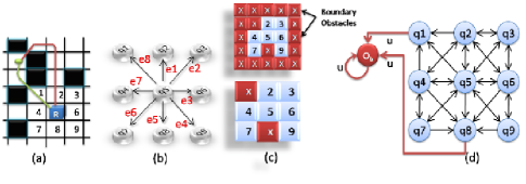
Figure 1: (a) shows the vehicle (marked ”R”) with the obstacle positions shown as black squares. The Green4 dot identifies the goal (b) shows the finite state representation of the possible one-step moves from the current position. (d) shows uncontrollable transitions ”u” from states corresponding to blocked grid locations to ”$q_{\circleddash}$”

We consider a 2D workspace for the mobile agents. This restriction on workspace dimensionality serves to simplify the exposition and can be easily relaxed. To set up the problem, the workspace is first discretized into a finite grid and hence the approach developed in this paper falls under the generic category of discrete planning. The underlying theory does not require the grid to be regular; however for the sake of clarity we shall present the formulation under the assumption of a regular grid. The obstacles are represented as blocked-off grid locations in the discretized workspace. We specify a particular location as the fixed goal and consider the problem of finding optimal and feasible paths from arbitrary initial grid locations in the workspace. Figure 1(a) illustrates the basic problem setup. We further assume that at any given time instant the robot occupies one particular location ($i.e.$ a particular square in Figure 1(a)). As shown in Figure 1, the robot has eight possible moves from any interior location. The boundaries are handled by removing the moves that take the robot out of the workspace. The possible moves are modeled as controllable transitions between grid locations since the robot can ”choose” to execute a particular move from the available set. We note that the number of possible moves ($8$ in this case) depends on the chosen fidelity of discretization of the robot motion and also on the intrinsic vehicle dynamics. The complexity results presented in this paper only assumes that the number of available moves is significantly smaller compared to the number of grid squares, $i.e.$, the discretized position states. Specification of inter-grid transitions in this manner allows us to generate a finite state automaton (FSA) description of the navigation problem. Each square in the discretized workspace is modeled as a FSA state with the controllable transitions defining the corresponding state transition map. The formal description of the model is as follows:

Let $\mathds{G}_{\textrm{{Nav}}}=(Q,\Sigma,\delta,\tilde{\Pi},\chi)$ be a Probabilistic Finite State Automaton (PFSA). The state set $Q$ consists of states that correspond to grid locations and one extra state denoted by $q_{\circleddash}$. The necessity of this special state $q_{\circleddash}$ is explained in the sequel. The grid squares are numbered in a pre-determined scheme such that each $q_{i}\in Q\setminus\{q_{\circleddash}\}$ denotes a specific square in the discretized workspace. The particular numbering scheme chosen is irrelevant. In the absence of dynamic uncertainties and state estimation errors, the alphabet contains one uncontrollable event $i.e.$ $\Sigma=\Sigma_{C}\bigcup\{u\}$ such that $\Sigma_{C}$ is the set of controllable events corresponding to the possible moves of the robot. The uncontrollable event $u$ is defined from each of the blocked states and leads to $q_{\circleddash}$ which is a deadlock state. All other transitions ($i.e.$ moves) are removed from the blocked states. Thus, if a robot moves into a blocked state, it uncontrollably transitions to the deadlock state $q_{\circleddash}$ which is physically interpreted to be a collision. We further assume that the robot fails to recover from collisions which is reflected by making $q_{\circleddash}$ a deadlock state. We note that $q_{\circleddash}$ does not correspond to any physical grid location. The set of blocked grid locations along with the obstacle state $q_{\circleddash}$ is denoted as $Q_{\textrm{{Obstacle}}}\subseteqq Q$. Figure 1 illustrates the navigation automaton for a nine state discretized workspace with two blocked squares. Note that the only outgoing transition from the blocked states $q_{1}$ and $q_{8}$ is $u$. Next we augment the navigation FSA by specifying event generation probabilities defined by the map $\tilde{\pi}:Q\times\Sigma\rightarrow[0,1]$ and the characteristic state-weight vector specified as $\chi:Q\rightarrow[-1,1]$. The characteristic state-weight vector [CR07] assigns scalar weights to the PFSA states to capture the desirability of ending up in each state.

Definition 13.

The characteristic weights are specified for the navigation automaton as follows:

$$\chi(q_{i})=\left\{\begin{array}[]{cl}-1&\mathrm{if}\ q_{i}\equiv q_{\circleddash}\\ 1&\mathrm{if}\ q_{i}\ \mathrm{is\ the\ goal}\\ 0&\mathrm{otherwise}\end{array}\right.$$ (6)

In the absence of dynamic constraints and state estimation uncertainties, the robot can ”choose” the particular controllable transition to execute at any grid location. Hence we assume that the probability of generation of controllable events is uniform over the set of moves defined at any particular state.

Definition 14.

Since there is no uncontrollable events defined at any of the unblocked states and no controllable events defined at any of the blocked states, we have the following consistent specification of event generation probabilities: $\forall q_{i}\in Q,\sigma_{j}\in\Sigma$,

$$\tilde{\pi}(q_{i},\sigma_{j}) =\left\{\begin{array}[]{cl}\frac{1}{\mathrm{No.\ of\ controllable\ events\ at\ }q_{i}},&\mathrm{if}\ \sigma_{j}\in\Sigma_{C}\\ 1,&\mathrm{otherwise}\end{array}\right.$$ (9)

The boundaries are handled by ”surrounding” the workspace with blocked position states shown as ”boundary obstacles” in the upper part of Figure 1(c).

Definition 15.

The navigation model id defined to have identical connectivity as far as controllable transitions are concerned implying that every controllable transition or move ($i.e.$ every element of $\Sigma_{C}$) is defined from each of the unblocked states.

2.4 Decision-theoretic Optimization of PFSA

The above-described probabilistic finite state automaton (PFSA) based navigation model allows us to compute optimally feasible path plans via the language-measure-theoretic optimization algorithm [CR07] described in Section 2. Keeping in line with nomenclature in the path-planning literature, we refer to the language-measure-theoretic algorithm as $\boldsymbol{\nu^{\star}}$ in the sequel. For the unsupervised model, the robot is free to execute any one of the defined controllable events from any given grid location (See Figure 1(b)). The optimization algorithm selectively disables controllable transitions to ensure that the formal measure vector of the navigation automaton is elementwise maximized. Physically, this implies that the supervised robot is constrained to choose among only the enabled moves at each state such that the probability of collision is minimized with the probability of reaching the goal simultaneously maximized. Although $\boldsymbol{\nu^{\star}}$ is based on optimization of probabilistic finite state machines, it is shown that an optimal and feasible path plan can be obtained that is executable in a purely deterministic sense.

Let $\mathds{G}_{\textrm{{Nav}}}$ be the unsupervised navigation automaton and $\mathds{G}_{\textrm{{Nav}}}^{\star}$ be the optimally supervised PFSA obtained by $\boldsymbol{\nu^{\star}}$. We note that $\nu_{\#}^{i}$ is the renormalized measure of the terminating plant $\mathds{G}_{\textrm{{Nav}}}^{\star}(\theta_{min})$ with substochastic event generation probability matrix $\widetilde{\Pi}^{\theta_{min}}=(1-\theta_{min})\widetilde{\Pi}$. Denoting the event generating function (See Definition 3) for $\mathds{G}_{\textrm{{Nav}}}^{\star}$ and $\mathds{G}_{\textrm{{Nav}}}^{\star}(\theta_{min})$ as $\tilde{\pi}:Q\times\Sigma\rightarrow Q$ and $\tilde{\pi}^{\theta_{min}}:Q\times\Sigma\rightarrow Q$ respectively, we have

$$\tilde{\pi}^{\theta_{min}}(q_{i},\epsilon)=1$$ (10a)

$$\forall q_{i}\in Q,\sigma_{j}\in\Sigma,\ \tilde{\pi}^{\theta_{min}}(q_{i},\sigma_{j})=(1-\theta_{min})\tilde{\pi}(q_{i},\sigma_{j})$$ (10b)

Notation 2.1.

For notational simplicity, we use

$$\nu_{\#}^{i}(L(q_{i}))=\nu_{\#}(q_{i})=\boldsymbol{\nu_{\#}}|_{i}$$

$$\mathrm{where}\ \boldsymbol{\nu_{\#}}=\theta_{min}[I-(1-\theta_{min})\Pi^{\#}]^{-1}\boldsymbol{\chi}$$

Definition 16 ($\boldsymbol{\nu^{\star}}$-path).

A $\boldsymbol{\nu^{\star}}$-path $\rho(q_{i},q_{j})$ from state $q_{i}\in Q$ to state $q_{j}\in Q$ is defined to be an ordered set of PFSA states $\rho=\{q_{r_{1}},\cdots,q_{r_{M}}\}$ with $q_{r_{s}}\in Q,\ \forall s\in\{1,\cdots,M\},M\leq\textrm{{Card}}(Q)$ such that

$$q_{r_{1}}=q_{i}$$ (11a)

$$q_{r_{M}}=q_{j}$$ (11b)

$$\forall i,j\in\{1,\cdots,M\},\ q_{r_{i}}\neq q_{r_{j}}$$ (11c)

$$\forall s\in\{1,\cdots,M\},\forall t\leqq s,\ \nu_{\#}(q_{r_{t}})\leqq\nu_{\#}(q_{r_{s}})$$ (11d)

We reproduce without proof the following key results pertaining to $\boldsymbol{\nu^{\star}}$- planning as reported in [CMR08].

Lemma 1.

There exists an enabled sequence of transitions from state $q_{i}\in Q\setminus Q_{\textrm{{Obstacle}}}$ to $q_{j}\in Q\setminus\{q_{\circleddash}\}$ in $\mathds{G}_{\textrm{{Nav}}}^{\star}$ if and only if there exists a $\boldsymbol{\nu^{\star}}$-path $\rho(q_{i},q_{j})$ in $\mathds{G}_{\textrm{{Nav}}}^{\star}$.

Proposition 1.

For the optimally supervised navigation automaton $\mathds{G}_{\textrm{{Nav}}}^{\star}$, we have

$$\forall q_{i}\in Q\setminus Q_{\textrm{{Obstacle}}},\ L(q_{i})\subseteqq\Sigma^{\star}_{C}$$

Corollary 1.

(Obstacle Avoidance:) There exists no $\boldsymbol{\nu^{\star}}$-path from any unblocked state to any blocked state in the optimally supervised navigation automaton $\mathds{G}_{\textrm{{Nav}}}^{\star}$.

Proposition 2 (Existence of $\boldsymbol{\nu^{\star}}$-paths).

There exists a $\boldsymbol{\nu^{\star}}$-path $\rho(q_{i},q_{\textrm{{Goal}}})$ from any state $q_{i}\in Q$ to the goal $q_{\textrm{{Goal}}}\in Q$ if and only if $\nu_{\#}(q_{i})>0$.

Corollary 2.

(Absence of Local Maxima:) If there exists a $\boldsymbol{\nu^{\star}}$-path from $q_{i}\in Q$ to $q_{j}\in Q$ and a $\boldsymbol{\nu^{\star}}$-path from $q_{i}$ to $q_{\textrm{{Goal}}}$ then there exists a $\boldsymbol{\nu^{\star}}$-path from $q_{j}$ to $q_{\textrm{{Goal}}}$, $i.e.$,

$$\forall q_{i},q_{j}\in Q\bigg{(}\exists\rho_{1}(q_{i},q_{\textrm{{Goal}}})\bigwedge\exists\rho_{2}(q_{i},q_{j})\Rightarrow\exists\rho(q_{j},q_{\textrm{{Goal}}})\bigg{)}$$

2.5 Optimal Tradeoff between Computed Path Length & Availability Of Alternate Routes

Figure 2: Tradeoff between path-length and robustness under dynamic uncertainty: $\sigma_{2}\omega$ is the shortest path to $q_{\textrm{{Goal}}}$ from $q_{i}$; but the $\boldsymbol{\nu^{\star}}$ plan may be $\sigma_{1}\omega_{1}$ due to the availability of larger number of feasible paths through $q_{j}$.

Majority of reported path planning algorithms consider minimization of the computed feasible path length as the sole optimization objective. However, the $\boldsymbol{\nu^{\star}}$ algorithm can be shown to achieve an optimal trade-off between path lengths and availability of feasible alternate routes. If $\omega$ is the shortest path to goal from state $q_{k}$, then the shortest path from state $q_{i}$ (with $q_{i}\xrightarrow{\sigma_{2}}q_{k}$) is given by $\sigma_{2}\omega$. However, a larger number of feasible paths may be available from state $q_{j}$ (with $q_{i}\xrightarrow{\sigma_{1}}q_{j}$) which may result in the optimal $\boldsymbol{\nu^{\star}}$ plan to be $\sigma_{1}\omega_{1}$. Mathematically, each feasible path from state $q_{j}$ has a positive measure which may sum to be greater than the measure of the single path $\omega$ from state $q_{k}$. The condition $\nu_{\#}(q_{j})>\nu_{\#}(q_{k})$ would then imply that the next state from $q_{i}$ would be computed to be $q_{j}$ and not $q_{k}$. Physically it can be interpreted that the mobile gent is better off going to $q_{j}$ since the goal remains reachable even if one or more paths become unavailable. The key results [CMR08] are as follows:

Lemma 2.

For the optimally supervised navigation automaton $\mathds{G}_{\textrm{{Nav}}}^{\star}$, we have $\forall q_{i}\in Q\setminus Q_{\textrm{{Obstacle}}}$,

$$\forall\omega\in L(q_{i}),\ \nu_{\#}^{i}(\{\omega\})=\theta_{min}\bigg{(}\frac{1-\theta_{min}}{\textrm{{Card}}(\Sigma_{C})}\bigg{)}^{|\omega|}\chi(\delta^{\#}(q_{i},\omega))$$

Proposition 3.

For $q_{i}\in Q\setminus Q_{\textrm{{Obstacle}}}$, let $q_{i}\xrightarrow{\sigma_{1}}q_{j}\rightarrow\cdots\rightarrow q_{\textrm{{Goal}}}$ be the shortest path to the goal. If there exists $q_{k}\in Q\setminus Q_{\textrm{{Obstacle}}}$ with $q_{i}\xrightarrow{\sigma_{2}}q_{k}$ for some $\sigma_{2}\in\Sigma_{C}$ such that $\nu_{\#}(q_{k})>\nu_{\#}(q_{j})$, then the number of distinct paths to goal from state $q_{k}$ is at least $\textrm{{Card}}(\Sigma_{C})+1$.

The lower bound computed in Proposition 3 is not tight and if the alternate paths are longer or if there are multiple ’shortest’ paths then the number of alternate routes required is significantly higher. Detailed examples can be easily presented to illustrate situation where $\boldsymbol{\nu^{\star}}$ opts for a longer but more robust plan.

3 Generalizing The Navigation Automaton To Accommodate Uncertain Execution

In this paper, we modify the PFSA-based navigation model to explicitly reflect uncertainties arising from imperfect localization and the dynamic response of the platform to navigation commands. These effects manifest as uncontrollable transitions in the navigation automaton as illustrated in Figure 4. Note, while in absence of uncertainties and dynamic effects, one can disable transitions perfectly, in the modified model, such disabling is only partial. Choosing the probabilities of the uncontrollable transitions correctly allows the model to incorporate physical movement errors and sensing noise in an amortized fashion.

A sample run with a SEGWAY RMP at NRSL is shown in Figure 3. Note that the robot is unable to follow the plan exactly due to cellular discretization and dynamic effects. Such effects can be conceptually modeled by decomposing trajectory fragments into sequential combinations of controllable and uncontrollable inter-cellular moves as illustrated in Figure 4(c). We do not need to actually decompose trajectories, it is merely a conceptual construct that gives us a theoretical basis for computing the probabilities of uncontrollable transitions from observed robot dynamics (as described later in Section 5, and therefore incorporate the amortized effect of uncertainties in the navigation automaton.

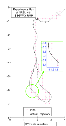
Figure 3: Plan execution with SEGWAY RMP at NRSL, Pennstate

\psfrag{J0}[tl]{$J_{0}$}\psfrag{J1}{}\psfrag{J2}{}\psfrag{J3}{}\psfrag{J4}[tc]{$J_{4}$}\psfrag{J5}{}\psfrag{J6}{}\psfrag{J7}[tl]{$J_{7}$}\psfrag{J8}{}\psfrag{T}[cc]{\small\color[rgb]{1,0,0}Trajectory}\psfrag{C}[cc]{\small\hbox{\hbox{\kern 0.0pt\raise-6.2pt\vbox{\halign{\relax\hfil\txtline@@{#}\hfil\cr\hbox{{\ignorespaces\leavevmode Controllable}\\\hbox{{\ignorespaces Move}\crcr}}}}}\psfrag{U}[cc]{\small\hbox{\hbox{\kern 0.0pt\raise-6.2pt\vbox{\halign{\relax\hfil\txtline@@{#}\hfil\cr\hbox{{\ignorespaces\leavevmode Uncontrollable }\\\hbox{{\ignorespaces Move}\crcr}}}}}\includegraphics[width=90.3375pt]{plan2}}}}}

Figure 4: (a) shows available moves from the current state (C) in unsupervised navigation automaton. (b) shows the enabled moves in the optimally supervised PFSA with no dynamic uncertainty, (c) illustrates the case with dynamic uncertainty, so that the robot can still uncontrollably (and hence unwillingly) make the disabled transitions, albeit with a small probability, $i.e.$, probability of transitions $e_{2}^{\prime},e_{3}^{\prime},e_{4}^{\prime}$ etc. is small. (d) illustrates the concept of using uncontrollable transitions to model dynamical response for a 2D circular robot: $J_{0}$ is the target cell from $J_{7}$, while the actual trajectory of the robot (shown in dotted line) ends up in $J_{4}$. We can model this trajectory fragment as first executing a controllable move to $J_{0}$ and then uncontrollably moving to $J_{4}$.

3.1 The Modified Navigation Automaton

The modified navigation automaton $\mathds{G}^{\textit{MOD}}_{\textrm{{Nav}}}=(Q,\Sigma,\delta,\widetilde{\Pi},\chi)$ is defined similar to the formulation in Section 2.3, with the exception that the alphabet $\Sigma$ is defined as follows:

$$\Sigma=\Sigma_{C}\cup\Sigma_{UC}\cup\{u\}$$ (12)

where $\Sigma_{C}$ is the set of controllable moves from any unblocked navigation state (as before), while $\Sigma_{UC}$ is the set of uncontrollable transitions that can occur as an effect of the platform dynamics and oather uncertainty effects. We assume that for each $\sigma\in\Sigma_{C}$, we have a corresponding event $\sigma_{u}$ in $\Sigma_{UC}$, such that both $\sigma$ and $\sigma_{u}$ represent the same physical move from a given navigation state; but while $\sigma$ is controllable and may be disabled, $\sigma_{u}$ is uncontrollable. Although for 2D circular robots we have: $\textrm{{Card}}(\Sigma_{C})=\textrm{{Card}}(\Sigma_{UC})$, in general, there can exist uncontrollable moves reflecting estimation errors that cannot be realized via a single controllable move. For example, for planar rectangular robots with a non-zero minimum turn radius, there can be an uncontrollable shift in the heading without any change in the $xy$-positional coordinates, which may reflect errors in heading estimation, but such a move cannot be executed via controllable transitions due to the restriction on the minimum turn radius. We will discuss these issues in more details in the sequel.

Definition 17.

The coefficient of dynamic deviation $\gamma(\mathds{G}^{\textit{MOD}}_{\textrm{{Nav}}})$ is defined as follows:

$$\gamma(\mathds{G}^{\textit{MOD}}_{\textrm{{Nav}}})=1-\max_{q_{i}\in Q}\sum_{\sigma_{u}\in\Sigma_{UC}}\tilde{\pi}(q_{i},\sigma_{u})$$ (13)

Definition 18.

The event generation probabilities for $\mathds{G}^{\textit{MOD}}_{\textrm{{Nav}}}$ is defined as follows: $\forall q_{i}\in Q\setminus\{q_{\textrm{{Goal}}}\},\sigma_{j}\in\Sigma$,

$$\tilde{\pi}(q_{i},\sigma_{j}) =\left\{\begin{array}[]{cl}\frac{1-\sum_{\sigma_{u}\in\Sigma_{UC}}\tilde{\pi}(q_{i},\sigma_{u})}{\mathrm{No.\ of\ controllable\ events\ at\ }q_{i}},&\mathrm{if}\ \sigma_{j}\in\Sigma_{C}\\ \tilde{\pi}(q_{i},\sigma_{j}),&\mathrm{if}\ \sigma_{j}\in\Sigma_{UC}\\ 1,&\mathrm{otherwise}\end{array}\right.$$ (17)

and for the goal, we define as before:

$$\tilde{\pi}(q_{\textrm{{Goal}}},\sigma_{j}) =\left\{\begin{array}[]{cl}\frac{1}{\mathrm{No.\ of\ controllable\ events\ at\ }q_{i}},&\mathrm{if}\ \sigma_{j}\in\Sigma_{C}\\ 1,&\mathrm{otherwise}\end{array}\right.$$ (20)

Note that we assume there is no uncontrollability at the goal. This assumption is made for technical reasons clarified in the sequel and also to reflect the fact that once we reach the goal, we terminate the mission and hence such effects can be neglected.

We note the following:

• In the idealized case where we assume platform dynamics is completely absent, we have $\tilde{\pi}(q_{i},\sigma_{u})=0,\forall q_{i}\in Q,\forall\sigma_{u}\in\Sigma_{UC}$ implying that $\gamma(\mathds{G}^{\textit{MOD}}_{\textrm{{Nav}}})=1$, while in practice, we expect $\gamma(\mathds{G}^{\textit{MOD}}_{\textrm{{Nav}}})<1$.

• In Definition 17, we allowed for the possibility of $\tilde{\pi}(q_{i},\sigma_{u})$ being dependent on the particular navigation states $q_{i}\in Q$. A significantly simpler approach would be to redefine the probability of the uncontrollable events $\tilde{\pi}(q_{i},\sigma_{u})$ as follows:

  $$\tilde{\pi}_{AV}(\sigma_{u})=\frac{1}{\textrm{{Card}}(Q)}\sum_{q_{i}\in Q}\tilde{\pi}(q_{i},\sigma_{u})$$ (21)

  where $\tilde{\pi}_{AV}(\sigma_{u})$ is the average probability of the uncontrollable event $\sigma_{u}$ being generated.

The averaging of the probabilities of uncontrollable transitions is justified in situations where we can assume that the dynamic response of the platform is not dependent on the location of the platform in the workspace. In this simplified case, the event generation probabilities for $\mathds{G}^{\textit{MOD}}_{\textrm{{Nav}}}$ can be stated as: $\forall q_{i}\in Q\setminus\{q_{\textrm{{Goal}}}\},\sigma_{j}\in\Sigma$,

$$\tilde{\pi}(q_{i},\sigma_{j}) =\left\{\begin{array}[]{cl}\frac{\gamma(\mathds{G}^{\textit{MOD}}_{\textrm{{Nav}}})}{\mathrm{No.\ of\ controllable\ events\ at\ }q_{i}},&\mathrm{if}\ \sigma_{j}\in\Sigma_{C}\\ \tilde{\pi}_{AV}(\sigma_{j}),&\mathrm{if}\ \sigma_{j}\in\Sigma_{UC}\\ 1,&\mathrm{otherwise}\end{array}\right.$$ (25)

The key difficulty is allowing the aforementioned dependence on states is not the decision optimization that would follow, but the complexity of identifying the probabilities; averaging results in significant simplification as shown in the sequel. Thus, even if we cannot realistically average out the uncontrollable transition probabilities over the entire state space, we could decompose the workspace to identify subregions where such an assumption is locally valid. In this paper, we do not address formal approaches to such decomposition, and will generally assume that the afore-mentioned averaging is valid throughout the workspace; the explicit identification of the sub-regions is more a matter of implementation specifics, and has little to do with the details of the planning algorithm presented here, and hence will be discussed elsewhere. In Section 5, we will address the computation of the probabilities of uncontrollable transitions from observed dynamics. First, we will establish the main planning algorithm as a solution to the performance optimization of the navigation automaton in the next section.

4 Optimal Planning Via Decision Optimization Under Dynamic Effects

The modified model $\mathds{G}^{\textit{MOD}}_{\textrm{{Nav}}}$ can be optimized via the measure-theoretic technique in a straightforward manner, using the $\boldsymbol{\nu^{\star}}$-algorithm reported in [CMR08]. The presence of uncontrollable transitions in $\mathds{G}^{\textit{MOD}}_{\textrm{{Nav}}}$ poses no problem (as far as the automaton optimization is concerned), since the underlying measure-theoretic optimization is already capable of handling such effects [CR07]. However the presence of uncontrollable transitions weakens some of the theoretical results obtained in [CMR08] pertaining to navigation, specifically the absence of local maxima. We show that this causes the $\boldsymbol{\nu^{\star}}$ planner to lose some of its crucial advantages, and therefore must be explicitly addressed via a recursive decomposition of the planning problem.

Proposition 4 (Weaker Version of Proposition 2).

There exists a $\boldsymbol{\nu^{\star}}$-path $\rho(q_{i},q_{\textrm{{Goal}}})$ from any state $q_{i}\in Q$ to the goal $q_{\textrm{{Goal}}}\in Q$ if $\nu_{\#}(q_{i})>0$.

Proof.

We note that $\nu_{\#}(q_{i})>0$ implies that there necessarily exists at least one string $\omega$ of positive measure initiating from $q_{i}$ and hence there exists at least one string that terminates on $q_{\textrm{{Goal}}}$. The proof then follows from the definition of $\boldsymbol{\nu^{\star}}$-paths (See Definition 16). ∎

Remark 2.

Comparing with Proposition 2, we note that the only if part of the result is lost in the modified case.

Remark 3.

We note that under the modified model, $\nu_{\#}(q_{i})<0$ needs to be interpreted somewhat differently. In absence of any dynamic uncertainty, $\nu_{\#}(q_{i})<0$ implies that no path to goal exists. However, due to weakening of Proposition 1 (See Proposition 4), $\nu_{\#}(q_{i})<0$ implies that the measure of the set of strings reaching the goal is smaller to that of the set of strings hitting an obstacle from the state $q_{i}$.

The $\boldsymbol{\nu^{\star}}$-planning algorithm is based on several abstract concepts such as the navigation automaton and the formal measure of symbolic strings. It is important to realize that in spite of the somewhat elaborate framework presented here, $\boldsymbol{\nu^{\star}}$-optimization is free from heuristics, which is often not the case with competing approaches. In this light, the next proposition is critically important as it elucidates this concrete physical connection.

\psfrag{N}[l]{\small No Connecting Path}\psfrag{G}[l][c]{\small\bf Goal}\psfrag{A}[c]{\small\bf A}\psfrag{B}[c]{\small\bf B}\psfrag{O}[l]{\small\bf Obstacles}\includegraphics[width=144.54pt,height=126.47249pt]{connectingpath}

Figure 5: Absence of uncontrollable transitions at the goal imply that there is no path in the optimally disabled navigation automaton from point A to point B (or vice versa), since all controllable transitions will necessarily be disabled at the goal. It follows that the stationary probability vector may be different depending on whether one starts left or right to the goal. However, note that that any two points on the same side have a path (possibly made of uncontrollable transitions) between them; implying that the stationary probability vector will be identical if either of them is chosen as the start locations.

Proposition 5.

Given that a feasible path exists from the starting state to the goal, the $\boldsymbol{\nu^{\star}}$ planning algorithm under non-trivial dynamic uncertainty ($i.e.$ with $\gamma(\mathds{G}^{\textit{MOD}}_{\textrm{{Nav}}})<1$) maximizes the probability $\wp_{\textrm{{Goal}}}$ of reaching the goal while simultaneously minimizing the probability $\wp_{\circleddash}$ of hitting an obstacle.

Proof.

Let $\wp$ be the stationary probability vector for the stochastic transition probability matrix corresponding to the navigation automaton $\mathds{G}^{\textit{MOD}}_{\textrm{{Nav}}}$, for a starting state from which a feasible path to goal exists. (Note that $\wp$ may depend on the starting state; Figure 5 illustrates one such example. However, once we fix a particular starting state, the stationary vector $\wp$ is uniquely determined). The selective disabling of controllable events modifies the transition matrix and in effect alters $\wp$, such that $\wp^{T}\chi$ is maximized [CR07], where $\boldsymbol{\chi}$ is the characteristic weight vector, $i.e.$ , $\boldsymbol{\chi}_{i}=\chi(q_{i})$. Recalling that $\chi(q_{\textrm{{Goal}}})=1,\chi(q_{\circleddash})=-1$ and $\chi(q_{i})=0$ if $q_{i}$ is neither the goal nor the abstract obstacle state $q_{\circleddash}$, we conclude that the optimization, in effect, maximizes the quantity:

$$\psi=\wp_{\textrm{{Goal}}}-\wp_{\circleddash}$$ (26)

Also, note that the optimized navigation automaton has only two dump states, namely the goal $q_{\textrm{{Goal}}}$ and the abstract obstacle state $q_{\circleddash}$. That the goal $q_{\textrm{{Goal}}}$ is in fact a dump state is ensured by not having uncontrollable transitions at the goal (See Definition 18). Hence we must have

$$\forall q_{i}\in Q\setminus\{q_{\textrm{{Goal}}},q_{\circleddash}\},\ \wp_{i}=0$$ (27)

implying that

$$\wp_{\textrm{{Goal}}}+\wp_{\circleddash}=1$$ (28a)

$$\Longrightarrow\psi=2\wp_{\textrm{{Goal}}}-1=1-2\wp_{\circleddash}$$ (28b)

Hence it follows that the optimization maximizes $\wp_{\textrm{{Goal}}}$ and simultaneously minimizes $\wp_{\circleddash}$. ∎

Remark 4.

It is easy to see that Proposition 5 remains valid if $\chi(q_{\textrm{{Goal}}})=\chi_{\textrm{{Goal}}}>1$. In fact, the result remains valid as long as the characteristic weight of the goal is positive and the characteristic weight of the abstract obstacle state $q_{\circleddash}$ is negative.

4.1 Recursive Problem Decomposition For Maxima Elimination

Weakening of Proposition 1 (See Proposition 4) has the crucial consequence that Corollary 2 is no longer valid. Local maxima can occur under the modified model. This is a serious problem for autonomous planning and must be remedied. The problem becomes critically important when applied to solution of mazes; larger the number of obstables, higher is the chance of ending up in a local maxima. While elimination of local maxima is notoriously difficult for potential based planning approaches, $\boldsymbol{\nu^{\star}}$ can be modified with ease into a recursive scheme that yields maxima-free plans in models with non-zero dynamic effects ($i.e.$ with $\gamma(\mathds{G}^{\textit{MOD}}_{\textrm{{Nav}}})<1$).

It will be shown in the sequel that for successful execution of the algorithm, we may need to assign a larger than unity characteristic weight $\chi_{\textrm{{Goal}}}$ to the goal $q_{\textrm{{Goal}}}$. A sufficient lower bound for $\chi_{\textrm{{Goal}}}$, with possible dependence on the recursion step, is given in Proposition 6. The basic recursion scheme can be described as follows (Also see the flowchart illustration in Algorithm 3):

1. In the first step ($i.e.$, at recursion step $k=1$) we execute $\boldsymbol{\nu^{\star}}$-optimization on the given navigation automaton $\mathds{G}^{\textit{MOD}}_{\textrm{{Nav}}}$ and obtain the measure vector $\boldsymbol{\nu_{\#}}^{[k]}$.

2. We denote the set of states with strictly positive measure as $Q_{k}$ ($k$ denotes the recursion step), $i.e.$,

   $$Q_{k}=\{q_{i}\in Q:\boldsymbol{\nu_{\#}}^{[k]}|_{i}>0\}$$ (29)

3. If $Q_{k}=Q_{k-1}$, the recursion terminates; else we update the characteristic weights as follows:

   $$\forall q_{i}\in Q_{k},\ \chi(q_{i})=\chi_{\textrm{{Goal}}}^{[k]}$$ (30)

   and continue the recursion by going back to the first step and incrementing the step number $k$.

\psfrag{P}[c]{\bf\small\hbox{\hbox{\kern 0.0pt\raise-7.922pt\vbox{\halign{\relax\hfil\txtline@@{#}\hfil\cr\hbox{{\ignorespaces\leavevmode\color[rgb]{.545,.145,0} Problem: }\\\hbox{{\ignorespaces$\mathds{G}^{\textit{MOD}}_{\textrm{{Nav}}}$}\crcr}}}}}\psfrag{E}[c]{\bf\small\color[rgb]{0,.545,0} Execute $\boldsymbol{\nu^{\star}}$}\psfrag{C}[c]{\bf\small$Q_{k}=Q_{k-1}?$}\psfrag{T}[c][c]{\bf\small Terminate}\psfrag{K}[l][c]{\bf\small Set $k=k+1$}\psfrag{S}[c]{\bf\small\hbox{\hbox{\kern 0.0pt\raise-8.12415pt\vbox{\halign{\relax\hfil\txtline@@{#}\hfil\cr\hbox{{\ignorespaces\leavevmode Save vector }\\\hbox{{\ignorespaces$\boldsymbol{\nu_{\#}}^{[k]}$}\crcr}}}}}\psfrag{G}[c]{\bf\small\hbox{\hbox{\kern 0.0pt\raise-18.75pt\vbox{\halign{\relax\hfil\txtline@@{#}\hfil\cr\hbox{{\ignorespaces\leavevmode 1. Set: $\forall q_{i}\in Q_{k}$}\\\hbox{{\ignorespaces$\chi(q_{i})=\chi_{\textrm{{Goal}}}^{[k]}$}\\\hbox{{\ignorespaces$\phantom{-}$2. Eliminate Uncont. }\\\hbox{{\ignorespaces transitions from }\\\hbox{{\ignorespaces all $q_{i}\in Q_{k}$}\crcr}}}}}\psfrag{Y}[c][c]{\bf\small\color[rgb]{.545,.145,0} No}\psfrag{N}[c][c]{\bf\small\color[rgb]{0,.408,.545}Yes}\psfrag{Q}[cc]{\bf\small\hbox{\hbox{\kern 0.0pt\raise-9.04166pt\vbox{\halign{\relax\hfil\txtline@@{#}\hfil\cr\hbox{{\ignorespaces\leavevmode$\phantom{XXXXXXXXX}$Define: }\\\hbox{{\ignorespaces$\phantom{XXXXXXXXXXX}$ $Q_{k}=\{q_{i}\in Q:\boldsymbol{\nu_{\#}}^{[k]}|_{i}>0\}$}\crcr}}}}}\psfrag{I}[l]{\bf\small\hbox{\hbox{\kern 0.0pt\raise-8.125pt\vbox{\halign{\relax\hfil\txtline@@{#}\hfil\cr\hbox{{\ignorespaces\leavevmode Initialize: }\\\hbox{{\ignorespaces$k=0,\ Q_{0}=\{q_{\textrm{{Goal}}}\}$}\crcr}}}}}\includegraphics[width=216.81pt]{flow}}}}}}}}}}}}}}

Algorithm 3 Flowchart for recursive $\boldsymbol{\nu^{\star}}$-planning

Proposition 6.

If $\theta_{min}^{[k]}$ is the critical termination probability (See Definition 11) for the $\boldsymbol{\nu^{\star}}$-optimization in the $k^{th}$ recursion step of Algorithm 3, then the following condition

$$\chi_{\textrm{{Goal}}}^{[k]}>\frac{\textrm{{Card}}(\Sigma_{C})}{1-\theta_{min}^{[k]}}\left(\frac{1}{\gamma}-1\right)$$ (31)

is sufficient to guarantee that the following statements are true:

1. If there exists a state $q_{i}\in Q\setminus Q_{k}$ from which at least one state $q_{\ell}\in Q_{k}$ is reachable in one hop, then $\boldsymbol{\nu_{\#}}^{[k]}|_{i}>0$.

2. The recursion terminates in at most $\textrm{{Card}}(Q)$ steps.

3. For the $k^{th}$ recursion step, either $Q_{k}\supsetneqq Q_{k-1}$ or no feasible path exists to $q_{\textrm{{Goal}}}$ from any state $q_{i}\in Q\setminus Q_{k-1}$.

\psfrag{G}[c][c]{\bf\small$q_{\textrm{{Goal}}}$}\psfrag{q}[c][c]{\bf\small$q_{i}$}\psfrag{p1}[c][t\trianglerighteq]{\bf\small$1-\theta_{min}$}\psfrag{p2}[c][c]{\bf\small$(1-\gamma)(1-\theta_{min})$}\psfrag{p3}[c][r]{\bf\small$(1-\theta_{min})\frac{\gamma}{\textrm{{Card}}(\Sigma_{C})}$}\psfrag{p4}[c][c]{\bf\small}\psfrag{a}[t][c]{\bf\small$q_{j}$}\psfrag{b}[t][c]{\bf\small$q_{k}$}\psfrag{O}[c][b]{\bf\small$q_{\circleddash}$ }\includegraphics[width=162.6075pt]{gneigh}

Figure 6: Illustration for Proposition 6. Uncontrollable events and strings are shown in dashed.

Proof.

Statement 1:
We first consider the first recursion step, $i.e.$, the case where $k=0$ and $Q_{k}=\{q_{\textrm{{Goal}}}\}$ (See Algorithm 3). We note that the goal $q_{\textrm{{Goal}}}$ achieves the maximum measure on account of the fact that only $q_{\textrm{{Goal}}}$ has a positive characteristic weight, $i.e.$, we have

$$\forall q_{i}\in Q,\ \boldsymbol{\nu_{\#}}^{[1]}|_{\textrm{{Goal}}}\geqq\boldsymbol{\nu_{\#}}^{[1]}|_{i}$$ (32)

It follows that all controllable transitions from the goal will be disabled in the optimized navigation automaton obtained at the end of the first recursion step (See Definition 8 and Algorithms 1 & 2), which in turn implies that the non-renormalized measure of the goal (at the end of the first recursion step) is given by $\chi_{\textrm{{Goal}}}\frac{1}{\theta_{min}}$.

The Hahn Decomposition Theorem [R88], allows us to write:

$$\boldsymbol{\nu_{\#}}|_{i}=\nu_{\#}(L^{+}(q_{i}))+\nu_{\#}(L^{-}(q_{i}))$$ (33)

where $L^{+}(q_{i}),L^{-}(q_{i})$ are the sets of strings initiating from state $q_{i}$ that have positive and negative measures respectively.

Let $q_{i}\in Q\setminus\{q_{\textrm{{Goal}}}\}$ such that $q_{\textrm{{Goal}}}$ is reachable from $q_{i}$ in one hop. We note that since it is possible to reach the goal in one hop from $q_{i}$, we have:

$$\nu_{\#}(L^{+}(q_{i}))\geqq\theta_{min}\times\frac{\gamma(1-\theta_{min})}{\textrm{{Card}}(\Sigma_{C})}\times\frac{\chi_{\textrm{{Goal}}}}{\theta_{min}}$$ (34)

where the first term arises due to renormalization (See Definition 7), the second term denotes the probability of the transition leading to the goal and the third term is the non-renormalized measure of the goal itself (as argued above). Since it is obvious that the goal achieves the maximum measure, the transition to the goal will obviously be enabled in the optimized automaton, which justifies the second term. It is clear that there are many more strings of positive measure ($e.g.$ arising due to the self loops at the state $q_{i}$ that correspond to the disabled controllable events that do not transition to the goal from $q_{i}$) which are not considered in the above inequality (which contributes to making the left hand side even larger); therefore guaranteeing the correctness of the lower bound stated in Eq.(34).

Next, we compute a lower bound for $\nu_{\#}(L^{-}(q_{i}))$. To that effect, we consider an automaton $G^{\prime}$ identical to the navigation automaton at hand in ever respect, but the fact that the $q_{\textrm{{Goal}}}$ has zero characteristic. We denote the state corresponding to $q_{i}$ in this hypothesized automaton as $q_{i}^{\prime}$, and the set of al states in $G^{\prime}$ as $Q^{\prime}$. We claim that, after a measure-theoretic optimization ($i.e.$ after applying Algorithms 1 and 2), the measure of $q_{i}^{\prime}$, denoted as $\nu^{\star}(q_{i}^{\prime})$, satisfies:

$$\nu^{\star}(q_{i}^{\prime})\geqq-(1-\gamma)$$ (35)

To prove the claim in Eq. (35), we first note that denoting the renormalized measure vector for $G^{\prime}$ before any optimization as $\boldsymbol{\nu^{\prime}}$, the characteristic vector as $\chi^{\prime}$ and for any termination probability $\theta\in(0,1)$, we have:

$$||\boldsymbol{\nu^{\prime}}||_{\infty}=||\theta[\mathbb{I}-(1-\theta)\Pi]^{-1}\chi^{\prime}||_{\infty}\\ \leqq||\theta[\mathbb{I}-(1-\theta)\Pi]^{-1}||_{\infty}\times 1=1$$ (36)

which follows from the following facts:

1. For all $\theta\in(0,1]$, $\theta[\mathbb{I}-(1-\theta)\Pi]^{-1}$ is a row-stochastic matrix and therefore has unity infinity norm [CR06]

2. $||\chi^{\prime}||_{\infty}=1$, since all entries of $\chi^{\prime}$ are $0$ except for the state corresponding to the obstacle state in the navigation automaton, which has a characteristic of $-1$.

Since the only non-zero characteristic is $-1$, it follows that no state in $G^{\prime}$ can have a positive measure and we conclude from Eq. (36) that:

$$\forall q_{j}^{\prime}\in Q^{\prime},\ \nu(q_{j}^{\prime})\in[-1,0]$$ (37)

Note that $q_{i}^{\prime}$ is not blocked itself (since we chose $q_{i}$ such that a feasible 1-hop path to the goal exists from $q_{i}$). Next, we subject $G^{\prime}$ to the measure-theoretic optimization (See Algorithms 1 & 2), which disables all controllable transitions to the blocked states. In order to compute a lower bound on the optimized measure for the state $q_{i}^{\prime}$, (denoted by $\nu^{\star}(q_{i}^{\prime})$ ), we consider the worst case scenario where all neighboring states that can be reached from $q_{i}^{\prime}$ in single hops are blocked. Denoting the set of all such neighboring states of $q_{i}$ by $\mathcal{N}(q_{i}^{\prime})$, we have:

$$\nu^{\star}(q_{i}^{\prime})=\sum_{q_{j}^{\prime}\in\mathcal{N}(q_{i}^{\prime})}\Pi^{u}_{ij}\nu(q_{j}^{\prime})\geqq-1\times\sum_{q_{j}^{\prime}\in\mathcal{N}(q_{i}^{\prime})}\Pi^{u}_{ij}=-1\times(1-\gamma)$$ (38)

where $\Pi^{u}_{ij}$ is the probability of the uncontrollable transition from $q_{i}^{\prime}$ to the neighboring state $q_{j}^{\prime}$. Note that we can write Eq. (38) in the worst case scenario where each state in $\mathcal{N}(q_{i}^{\prime})$ is blocked, since all controllable transitions from $q_{i}^{\prime}$ will be disabled in the optimized plant under such a scenario, and only the uncontrollable transitions will remain enabled; and the probabilities of all uncontrollable transitions defined at state $q_{i}$ sums to $1-\gamma$. It is obvious that the lower bound computed in Eq. (38) also reflects a lower bound for $\nu_{\#}(L^{-}(q_{i}))$, since addition of state(s) with positive characteristic or eliminating obstacles cannot possibly make strings more negative. Furthermore, recalling that the goal $q_{\textrm{{Goal}}}$ is actually reachable from state $q_{i}$ by a single hop, it follows that not all neighbors of $q_{i}$ in the navigation automaton are blocked, and hence we have the strict inequality:

$$\nu_{\#}(L^{-}(q_{i}))>-(1-\gamma)$$ (39)

Combining Eqns. (34) and (39), we note that the following condition is sufficient for guaranteeing $\boldsymbol{\nu_{\#}}|_{i}>0$.

$$\frac{\gamma(1-\theta_{min})}{\textrm{{Card}}(\Sigma_{C})}\times\chi_{\textrm{{Goal}}}>1-\gamma$$ (40)

which after a straightforward calculation yields the bound stated in Eq. 31, and the Statement 1 is proved for the first recursion step, $i.e.$ for $Q_{k}=\{q_{\textrm{{Goal}}}\}$.

\psfrag{qi1}[c][c]{\bf$q_{i}$}\psfrag{qi2}[c][c]{\bf$q_{i}$}\psfrag{u}[c][c]{\bf$\sigma$}\psfrag{s1}[c][c]{\bf$\sigma_{1}$}\psfrag{s2}[c][c]{\bf$\sigma_{2}$}\psfrag{s21}[c][c]{\bf$\sigma_{1},\sigma_{2}$}\psfrag{Q}[c][c]{\bf\color[rgb]{.545,.145,0} $\boldsymbol{Q_{k}}$}\psfrag{qj3}[c][c]{\bf$q_{j_{1}}$}\psfrag{qj4}[c][c]{\bf$q_{j_{2}}$}\psfrag{qj5}[c][c]{\bf$q_{j_{3}}$}\psfrag{qj2}[c][c]{\bf$q_{\textrm{{Goal}}}$}\includegraphics[width=173.44756pt]{reduceGoal}

Figure 7: Illustration for Statement 1 of Proposition 6. Note that even if $Q_{k}$ has multiple states, $q_{j_{1}},q_{j_{2}},q_{j_{3}}$, the measure of any string (say $\sigma\sigma_{1}\sigma_{1}\sigma_{2}$) from $q_{i}$ is the same as if $q_{i}$ was directly connected to the goal $q_{\textrm{{Goal}}}$ with all controllable events disabled at $q_{\textrm{{Goal}}}$. The bottom plate illustrates this by showing the hypothetical scenario where $q_{i}$ is connected to $q_{\textrm{{Goal}}}$ by $\sigma$ and $\sigma_{1},\sigma_{2}$ are controllable events disabled at $q_{\textrm{{Goal}}}$. Note that for this argument to work, we must eliminate uncontrollable transitions from all states in $Q_{k}$.

To extend the argument to later recursion steps of Algorithm 3, $i.e.$, for $k>0$, we argue as follows. Let $Q_{k}\supsetneqq\{q_{\textrm{{Goal}}}\}$ and we have eliminated all uncontrollable transitions from all $q_{j}\in Q_{k}$ (as required in Algorithm 3). Further, let $q_{i}\in Q\setminus Q_{k}$ such that it is possible to reach some $q_{j}\in Q$ in a single controllable hop, $i.e.$

$$q_{i}\xrightarrow[controllable]{\sigma}q_{j},\ q_{j}\in Q_{k}$$ (41)

We first claim that

$$\forall q_{j}\in Q_{k},q_{r}\notin Q_{k},\ \boldsymbol{\nu_{\#}}^{[k]}|_{j}>\boldsymbol{\nu_{\#}}^{[k]}|_{r}$$ (42)

which immediately follows from the fact that the optimal configuration (of transitions from states in $Q_{k}$) at the end of the $\boldsymbol{\nu^{\star}}$-optimization at the $k^{th}$ step would be to have all controllable transitions from states $q_{j}\in Q_{k}$ enabled if and only if the transition goes to some state in $Q_{k}$, since in that case every string initiating from $q_{j}$ terminates on a state having characteristic $\chi_{\textrm{{Goal}}}$ (since there is no uncontrollability from states within $Q_{k}$ by construction), whereas if a transition $q_{j}\xrightarrow[controllable]{\sigma}q_{r},\ \mathrm{where}\ q_{j}\in Q_{k},q_{r}\notin Q_{k}$ allows strings which end up in zero-characteristic states and also (via uncontrollable transitions) on negative-characteristic states.

Eq.  (42) implies that no enabled string exits $Q_{k}$. It therefore follows that every string $\sigma\omega$ starting from the state $q_{i}$, with $\omega\in\Sigma_{C}^{\star}$ and $\delta(q_{i},\sigma)\in Q_{k}$ ($i.e.$, $\sigma$ leads to some state within $Q_{k}$) has exactly the same measure as if $q_{i}$ is directly connected to $q_{\textrm{{Goal}}}$ and all controllable transitions are disabled at $q_{\textrm{{Goal}}}$ (See Figure 7 for an illustration). This conceptual reduction implies that Eq. (34) is valid when $Q_{k}\supsetneqq\{q_{\textrm{{Goal}}}\}$ since the lower bound for $\nu_{\#}(L^{+}(q_{i}))$ can be computed exactly as already done for the case with $Q_{k}=\{q_{\textrm{{Goal}}}\}$. The argument for obtaining the lower bound for $\nu_{\#}(L^{-}(q_{i}))$ is the same as before, thus completing the proof for Statement 1 for all recursion steps of Algorithm 3 .
Statement 2:
Let $Q_{R}\subsetneqq Q$ be the set of states from which a feasible path to the goal exists. If $\textrm{{Card}}(Q_{R})=1$, then we must have $Q_{R}=\{q_{\textrm{{Goal}}}\}$ and the recursion terminates in one step. In general, for the $k^{th}$ recursion step, let $\textrm{{Card}}(Q_{k})<\textrm{{Card}}(Q_{R})$. Since there exists at least one state, not in $Q_{k}$, from which a feasible path to the goal exists, it follows that there exists at least one state $q_{j}$ from which it is possible to reach a state in $Q_{k}$ in one hop. Using Statement 1, we can then conclude:

$$Q_{k+1}\neq Q_{k}\Rightarrow\textrm{{Card}}(Q_{k+1})\geqq\textrm{{Card}}(Q_{k})+1$$

$$\Rightarrow\textrm{{Card}}(Q_{k+1})\geqq k+1$$ (43)

which immediately implies that the recursion must terminate in at most $\textrm{{Card}}(Q)$ steps.
Statement 3:
Follows immediately from the argument used for proving Statement 2. ∎

Remark 5.

The generality of Eq. (31) is remarkable. Note that the lower bound is not directly dependent on the exact structure of the navigation automaton; what only matters is the number of controllable moves available at each state, the coefficient of dynamic deviation $\gamma(\mathds{G}^{\textit{MOD}}_{\textrm{{Nav}}})$ and the critical termination probability $\theta_{min}$. Although the exact automaton structure and the probability distribution of the uncontrollable transitions are not directly important, their effect enters, in a somewhat non-trivial fashion, through the value of the critical termination probability. The reader might want to review Algorithm 2 (See also [CR06, CR07]) which computes the critical termination probability in each step of the $\boldsymbol{\nu^{\star}}$-optimization for a better elucidation of the aforementioned connection between the structure of the navigation automaton and $\chi_{\textrm{{Goal}}}$.

The dependencies of the acceptable lower bound for $\chi_{\textrm{{Goal}}}$ with the coefficient of dynamic deviation $\gamma(\mathds{G}^{\textit{MOD}}_{\textrm{{Nav}}})$, as computed in Proposition 6, is illustrated in Figures 8(a) and (b). The key points to be noted are:

1. As $\gamma(\mathds{G}^{\textit{MOD}}_{\textrm{{Nav}}})\rightarrow 0^{+}$, $\chi_{\textrm{{Goal}}}\rightarrow+\infty$; which reflects the physical fact that if no events are controllable, then we cannot optimize the mission plan no matter how large $\chi_{\textrm{{Goal}}}$ is chosen.

2. As $\gamma(\mathds{G}^{\textit{MOD}}_{\textrm{{Nav}}})\rightarrow 1$, $\chi_{\textrm{{Goal}}}\rightarrow 0$; which implies that in the absence of dynamic effects any positive value of $\chi_{\textrm{{Goal}}}$ suffices. This reiterates the result obtained with $\chi_{\textrm{{Goal}}}=1$ in [CMR08].

3. As the number of available controllable moves increases (See Figure 8(a)), we need a larger value of $\chi_{\textrm{{Goal}}}$; similarly if the critical termination probability $\theta_{min}$ is large, then the value of $\chi_{\textrm{{Goal}}}$ required is also large (See Figure 8(b)).

4. The functional relationships in Figures 8(a) and (b) establish the fact that for relatively smaller number of controllable moves, a large value of $\gamma(\mathds{G}^{\textit{MOD}}_{\textrm{{Nav}}})$ and a small termination probability, a constant value of $\chi_{\textrm{{Goal}}}=1$ may be sufficient.

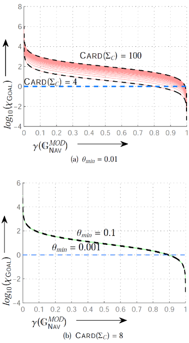
Figure 8: Variation of the acceptable lower bound for $\chi_{\textrm{{Goal}}}$ with $\gamma(\mathds{G}^{\textit{MOD}}_{\textrm{{Nav}}})$. (a) The set of controllable moves is expanded from $\textrm{{Card}}(\Sigma_{C})=4$ to $\textrm{{Card}}(\Sigma_{C})=100$ while holding $\theta_{min}=0.01$ (b) The critical termination probability $\theta_{min}$ is varied from $0.001$ to $0.1$ while holding $\textrm{{Card}}(\Sigma_{C})=8$. Note the lines are almost coincident in this case.

input : $\boldsymbol{\nu_{\#}}^{[k]},k=1,\cdots,K$

(Plan Vectors) output : $\boldsymbol{\nu_{\#}}^{\mathbf{A}}$ (Assembled Plan)

begin  Set $\boldsymbol{\nu_{\#}}^{\mathbf{A}}=\boldsymbol{0}$;  /* Zero vector */

for $k=1:K$ do  for $i\in Q$ do  $\boldsymbol{\nu_{\#}}^{tmp}|_{i}=0$; AlgoLine0.1

if $\boldsymbol{\nu_{\#}}^{[k-1]}|_{i}>0$ then  $\boldsymbol{\nu_{\#}^{tmp}}|_{i}=1$; AlgoLine0.2

else  if $\boldsymbol{\nu_{\#}}^{[k]}|_{i}>0$ then  $\boldsymbol{\nu_{\#}^{tmp}}|_{i}=\boldsymbol{\nu_{\#}}^{[k]}|_{i}$; AlgoLine0.3

endif endif endfor $\boldsymbol{\nu_{\#}}^{\mathbf{A}}=\boldsymbol{\nu_{\#}}^{\mathbf{A}}+\boldsymbol{\nu_{\#}^{tmp}}$;AlgoLine0.4

endfor endAlgoLine0.5

Algorithm 4 Assembly of Plan Vectors

5

5

5

5

5

4.2 Plan Assembly & Execution Approach

The plan vectors $\boldsymbol{\nu_{\#}}^{[k]}$ (Say, there are $K$ of them, $i.e.$, $k\in\{1,\cdots,K\}$) obtained via the recursive planning algorithm described above, can be used for subsequent mission execution in two rather distinct ways:

1. (The Direct Approach:)

   • At any point during execution, if the current state $q_{i}\in Q_{k}$ for some $k\in\{1,\cdots,K\}$, then use the gradient defined by the plan vector $\boldsymbol{\nu_{\#}}^{[k]}$ to decide on the next move, $i.e.$, $q_{j}$ is an acceptable next state if $\boldsymbol{\nu_{\#}}^{[k]}|_{j}>\boldsymbol{\nu_{\#}}^{[k]}|_{i}$ and for states $q_{\ell}$ that can be reached from the current state $q_{i}$ via controllable events, we have $\boldsymbol{\nu_{\#}}^{[k]}|_{j}\geqq\boldsymbol{\nu_{\#}}^{[k]}|_{\ell}$.

   • if $\forall k\in\{1,\cdots,K\},\ q_{i}\notin Q_{k}$, then terminate operation because there is no feasible path to the goal.

   • Note that this entails keeping $K$ vectors in memory.

2. (The Assembled Plan Approach:)

   • Use $\boldsymbol{\nu_{\#}}^{[k]},k\in\{1,\cdots,K\}$ to obtain the assembled plan vector $\boldsymbol{\nu_{\#}}^{\mathbf{A}}$ following Algorithm 4, which assigns a real value $\boldsymbol{\nu_{\#}}^{\mathbf{A}}|_{i}$ to each state $q_{i}$ in the workspace. We refer to this map as the assembled plan.

   • Make use of the gradient defined by $\boldsymbol{\nu_{\#}}^{\mathbf{A}}$ to reach the goal, by sequentially moving to states with increasing values specified by the assembled plan, $i.e.$,. if the current state is $q_{i}\in Q$, then $q_{j}$ is an acceptable next state if $\boldsymbol{\nu_{\#}}^{\mathbf{A}}|_{j}>\boldsymbol{\nu_{\#}}^{\mathbf{A}}|_{i}$ and for states $q_{\ell}$ that can be reached from the current state $q_{i}$ via controllable events, we have $\boldsymbol{\nu_{\#}}^{\mathbf{A}}|_{j}\geqq\boldsymbol{\nu_{\#}}^{\mathbf{A}}|_{\ell}$.

   • We show in the sequel that if $\boldsymbol{\nu_{\#}}^{\mathbf{A}}|_{i}<0$, then no feasible path exists to the goal.

Before we can proceed further, we need to formally establish some key properties of the assembled plan approach. In particular, we have the following proposition:

Proposition 7.

1. For a state $q_{i}\in Q$, a feasible path to the goal exists from the state $q_{i}$, if and only if $\boldsymbol{\nu_{\#}}^{\mathbf{A}}|_{i}>0$.

2. The assembled plan $\boldsymbol{\nu_{\#}}^{\mathbf{A}}$ is free from local maxima, $i.e.$, if there exists a $\boldsymbol{\nu^{\star}}$-path (w.r.t. to $\boldsymbol{\nu_{\#}}^{\mathbf{A}}$) from $q_{i}\in Q$ to $q_{j}\in Q$ and a $\boldsymbol{\nu^{\star}}$-path from $q_{i}$ to $q_{\textrm{{Goal}}}$ then there exists a $\boldsymbol{\nu^{\star}}$-path from $q_{j}$ to $q_{\textrm{{Goal}}}$, $i.e.$,

   $$\forall q_{i},q_{j}\in Q\bigg{(}\exists\rho_{1}(q_{i},q_{\textrm{{Goal}}})\bigwedge\exists\rho_{2}(q_{i},q_{j})\Rightarrow\exists\rho(q_{j},q_{\textrm{{Goal}}})\bigg{)}$$

3. If a feasible path to the goal exists from the state $q_{i}$, then the agent can reach the goal optimally by following the gradient of $\boldsymbol{\nu_{\#}}^{\mathbf{A}}$, where the optimality is to be understood as maximizing the probability of reaching the goal while simultaneously minimizing the probability of hitting an obstacle ($i.e.$ in the sense stated in Proposition 5).

Proof.

Statement 1:
Let the plan vectors obtained by the recursive procedure stated in the previous section be $\boldsymbol{\nu_{\#}}^{[k]}$ (Say, there are $K$ of them, $i.e.$, $k\in\{1,\cdots,K\}$) and further let the current state $q_{i}\in Q_{k}$ for some $k\in\{1,\cdots,K\}$. We observe that on account of Proposition 4, if $k=1$, then $\boldsymbol{\nu_{\#}}^{[k]}|_{i}>0$ is sufficient to guarantee that there exists a $\boldsymbol{\nu^{\star}}$-path $\rho(q_{i},q_{\textrm{{Goal}}})$ w.r.t the plan vector $\boldsymbol{\nu_{\#}}^{[1]}$. We further note that $\boldsymbol{\nu_{\#}}^{[1]}|_{i}<=0\Rightarrow q_{i}\notin Q_{1}$ (See Eq. (29)), implying that $\boldsymbol{\nu_{\#}}^{[1]}|_{i}>0$ is also necessary for the existence of $\rho(q_{i},q_{\textrm{{Goal}}})$. Extending this argument, we note that, for $k>1$, a $\boldsymbol{\nu^{\star}}$-path $\rho(q_{i},q_{j})$ with $q_{j}\in Q_{k-1}$ exists (with respect to the plan vector $\boldsymbol{\nu_{\#}}^{[k]}$) if and only if $\boldsymbol{\nu_{\#}}^{[k]}|_{i}>0$. Noting that $\boldsymbol{\nu_{\#}}^{[k]}|_{i}>0\Leftrightarrow\boldsymbol{\nu_{\#}}^{\mathbf{A}}|_{i}>0$, (See Algorithm 4) we conclude that a $\boldsymbol{\nu^{\star}}$-path $\rho(q_{i},q_{j})$ with $q_{j}\in Q_{k-1}$ exists (with respect to the plan vector $\boldsymbol{\nu_{\#}}^{[k]}$) if and only if $\boldsymbol{\nu_{\#}}^{\mathbf{A}}|_{i}>0$. Also, since $q_{j}\in Q_{k-1}\wedge q_{i}\in Q_{k}$, it follows from Algorithm 4, that $\boldsymbol{\nu_{\#}}^{\mathbf{A}}|_{j}\geqq 1+\boldsymbol{\nu_{\#}}^{\mathbf{A}}|_{i}>0$. It follows that the same argument can be used recursively to find $\boldsymbol{\nu^{\star}}$-paths $\rho(q_{j},q_{\ell_{1}}),\cdots,\rho(q_{j},q_{\textrm{{Goal}}})$ if and only if $\boldsymbol{\nu_{\#}}^{\mathbf{A}}|_{i}>0$.

To complete the proof, we still need to show that if there exists a feasible path from a state $q_{i}$ to the goal $q_{\textrm{{Goal}}}$, then there exists a $\boldsymbol{\nu^{\star}}$-path $\rho(q_{i},q_{\textrm{{Goal}}})$. We argue as follows: Let $q_{i}=q_{r1}\rightarrow q_{r2}\rightarrow\cdots\rightarrow q_{r_{m-1}}\rightarrow q_{r_{m}}=q_{\textrm{{Goal}}}$ be a feasible path from the state $q_{i}$ to $q_{\textrm{{Goal}}}$. Furthermore, assume if possible that

$$\forall k\ \boldsymbol{\nu_{\#}}^{[k]}|_{i}\leqq 0$$ (44)

$i.e.$, there exists no $\boldsymbol{\nu^{\star}}$-path from $q_{i}$ to $q_{\textrm{{Goal}}}$ w.r.t $\boldsymbol{\nu_{\#}}^{\mathbf{A}}$. We observe that since it is possible to reach $q_{\textrm{{Goal}}}$ from $q_{r_{m-1}}$ in one hop, using Proposition 6 we have:

$$\boldsymbol{\nu_{\#}}^{[1]}|_{r_{m-1}}>0\Rightarrow q_{r_{m-1}}\in Q_{1}$$ (45)

We further note:

$$\boldsymbol{\nu_{\#}}^{[1]}|_{r_{m-2}}>0\Rightarrow q_{r_{m-2}}\in Q_{1}$$ (46)

$$\boldsymbol{\nu_{\#}}^{[1]}|_{r_{m-2}}\leqq 0\Rightarrow\boldsymbol{\nu_{\#}}^{[2]}|_{r_{m-2}}>0\Rightarrow q_{r_{m-2}}\in Q_{2}$$ (47)

Hence, we conclude either $q_{r_{m-2}}\in Q_{2}$ or $q_{r_{m-2}}\in Q_{1}$. It follows by straightforward induction that either $q_{1}\in Q_{m-1}$ or $q_{1}\in Q_{m-2}$, which contradicts the statement in Eq. (44). Therefore, we conclude that if a feasible path to the goal exists from any state $q_{i}$, then a $\boldsymbol{\nu^{\star}}$-path $\rho(q_{i},q_{\textrm{{Goal}}})$ (w.r.t $\boldsymbol{\nu_{\#}}^{\mathbf{A}}$) exists as well. This completes the proof of Statement 1.
Statement 2:
Given states $q_{i},q_{j}\in Q$, assume that we have the $\boldsymbol{\nu^{\star}}$-paths $\rho_{1}(q_{i},q_{\textrm{{Goal}}})$ and $\rho_{2}(q_{i},q_{j})$. We observe that:

$$\exists\rho_{1}(q_{i},q_{\textrm{{Goal}}})\Rightarrow\boldsymbol{\nu_{\#}}^{\mathbf{A}}|_{i}>0\ \mathsf{(See\ Statement\ 1)}$$ (48a)

$$\exists\rho_{2}(q_{i},q_{j})\Rightarrow\boldsymbol{\nu_{\#}}^{\mathbf{A}}|_{j}\geqq\boldsymbol{\nu_{\#}}^{\mathbf{A}}|_{i}\ \mathsf{(See\ Definition~{}\ref{defnustar})}$$ (48b)

$$\Rightarrow\boldsymbol{\nu_{\#}}^{\mathbf{A}}|_{j}>0\Rightarrow\exists\rho(q_{j},q_{\textrm{{Goal}}})\ \mathsf{(See\ Statement\ 1)}$$ (48c)

which proves Statement 2.
Statement 3:
Statements 1 and 2 guarantee that if a feasible path to the goal exists from a state $q_{i}\in Q$, then an agent can reach the goal by following a $\boldsymbol{\nu^{\star}}$-path (w.r.t $\boldsymbol{\nu_{\#}}^{\mathbf{A}}$) from $q_{i}$, $i.e.$, by sequentially moving to states which have a better measure as compared to the current state.

We further note that a $\boldsymbol{\nu^{\star}}$-path $\omega$ w.r.t $\boldsymbol{\nu_{\#}}^{\mathbf{A}}$ from any state $q_{i}$ to $q_{\textrm{{Goal}}}$ can be represented as a concatenated sequence $\omega_{1}\omega_{2}\cdots\omega_{r}\cdots\omega_{m}$ where $\omega_{r}$ is a $\boldsymbol{\nu^{\star}}$-path from some intermediate state $q_{j}\in Q_{s}$, for some $s\in\{1,\cdots,K\}$, to some state $q_{\ell}\in Q_{s-1}$. Since the recursive procedure optimizes all such intermediate plans, and since the outcome “reached goal from $q_{i}$” can be visualized as the intersection of the mutually independent outcomes “reached $Q_{s}$ from $q_{i}\in Q_{s-1}$”, “reached $Q_{s+1}$ from $q_{j}\in Q_{s}$” , $\cdots$ , “reached $q_{\textrm{{Goal}}}$ from $q_{\ell}\in Q_{1}$”, the overall path must be optimal as well. This completes the proof. ∎

We compute the set of acceptable next states from the following definition.

Definition 19.

Given the current state $q_{i}\in Q$, $Q_{next}$ is the set of states satisfying the strict inequality:

$$Q_{next}=\{q_{j}\in Q:\boldsymbol{\nu_{\#}}^{\mathbf{A}}|_{j}>\boldsymbol{\nu_{\#}}^{\mathbf{A}}|_{i}\}$$ (49)

We note that Proposition 7 implies that $Q_{next}$ is empty if and only if the current state is the goal or if no feasible path to the goal exists from the current state.

5 Computation of Amortized Uncertainty Parameters

\psfrag{U}[cc]{\bf\footnotesize\color[rgb]{0,.408,.545} \hbox{\hbox{\kern 0.0pt\raise-6.2889pt\vbox{\halign{\relax\hfil\txtline@@{#}\hfil\cr\hbox{{\ignorespaces\leavevmode Actuation \& Localization }\\\hbox{{\ignorespaces Uncertainty}\crcr}}}}}\psfrag{G}[ct]{\bf\scriptsize\color[rgb]{0,.545,0}\hbox{\hbox{\kern 0.0pt\raise-3.1111pt\vbox{\halign{\relax\hfil\txtline@@{#}\hfil\cr\hbox{{\ignorespaces\leavevmode Grid Decomposition}\crcr}}}}}\psfrag{R}[cc]{\bf\scriptsize\color[rgb]{1,1,1} R}\psfrag{T}[lt]{\bf\footnotesize\color[rgb]{0,.408,.545}Trajectory}\psfrag{q1}[cc]{\bf\footnotesize\color[rgb]{0,.545,0} $\phantom{|}q_{1}$}\psfrag{q2}[cc]{\bf\footnotesize\color[rgb]{0,.545,0} $\phantom{|}q_{2}$}\psfrag{q3}[cc]{\bf\footnotesize\color[rgb]{0,.545,0} $\phantom{|}q_{3}$}\psfrag{q4}[cc]{\bf\footnotesize\color[rgb]{0,.545,0} $\phantom{|}q_{4}$}\psfrag{q5}[cc]{\bf\footnotesize\color[rgb]{0,.545,0} $\phantom{|}q_{5}$}\psfrag{q6}[cc]{\bf\footnotesize\color[rgb]{0,.545,0} $\phantom{|}q_{6}$}\psfrag{q7}[cc]{\bf\footnotesize\color[rgb]{0,.545,0} $\phantom{|}q_{7}$}\psfrag{q8}[cc]{\bf\footnotesize\color[rgb]{0,.545,0} $\phantom{|}q_{8}$}\psfrag{Q}[cc]{\bf\footnotesize\color[rgb]{0,.545,0} $\phantom{|}Q$}\includegraphics[width=252.94499pt]{uncertain}}}}

\psfrag{U}[cc]{\bf\footnotesize\color[rgb]{0,.408,.545} \hbox{\hbox{\kern 0.0pt\raise-6.2889pt\vbox{\halign{\relax\hfil\txtline@@{#}\hfil\cr\hbox{{\ignorespaces\leavevmode Actuation \& Localization }\\\hbox{{\ignorespaces Uncertainty}\crcr}}}}}\psfrag{G}[ct]{\bf\scriptsize\color[rgb]{0,.545,0}\hbox{\hbox{\kern 0.0pt\raise-3.1111pt\vbox{\halign{\relax\hfil\txtline@@{#}\hfil\cr\hbox{{\ignorespaces\leavevmode Grid Decomposition}\crcr}}}}}\psfrag{R}[cc]{\bf\scriptsize\color[rgb]{1,1,1} R}\psfrag{T}[lt]{\bf\footnotesize\color[rgb]{0,.408,.545}Trajectory}\psfrag{q1}[cc]{\bf\footnotesize\color[rgb]{0,.545,0} $\phantom{|}q_{1}$}\psfrag{q2}[cc]{\bf\footnotesize\color[rgb]{0,.545,0} $\phantom{|}q_{2}$}\psfrag{q3}[cc]{\bf\footnotesize\color[rgb]{0,.545,0} $\phantom{|}q_{3}$}\psfrag{q4}[cc]{\bf\footnotesize\color[rgb]{0,.545,0} $\phantom{|}q_{4}$}\psfrag{q5}[cc]{\bf\footnotesize\color[rgb]{0,.545,0} $\phantom{|}q_{5}$}\psfrag{q6}[cc]{\bf\footnotesize\color[rgb]{0,.545,0} $\phantom{|}q_{6}$}\psfrag{q7}[cc]{\bf\footnotesize\color[rgb]{0,.545,0} $\phantom{|}q_{7}$}\psfrag{q8}[cc]{\bf\footnotesize\color[rgb]{0,.545,0} $\phantom{|}q_{8}$}\psfrag{Q}[cc]{\bf\footnotesize\color[rgb]{0,.545,0} $\phantom{|}Q$}\psfrag{X}[rb]{\footnotesize\bf X}\psfrag{Y}[rb]{\footnotesize\bf Y}\psfrag{A}[lt]{\footnotesize\bf A}\psfrag{B}[rb]{\footnotesize\bf B}\psfrag{C}[rb]{\footnotesize\bf C}\psfrag{D}[lt]{\footnotesize\bf D}\psfrag{j0}{\small$J_{0}$}\psfrag{j1}{\small$J_{1}$}\psfrag{j2}{\small$J_{2}$}\psfrag{j3}{\small$J_{3}$}\psfrag{j4}[ct]{\small$J_{4}$}\psfrag{j5}[ct]{\small$J_{5}$}\psfrag{j6}[ct]{\small$J_{6}$}\psfrag{j7}{\small$J_{7}$}\psfrag{j8}{\small$J_{8}$}\psfrag{p}[cb]{\small\hbox{\hbox{\kern 0.0pt\raise-3.075pt\vbox{\halign{\relax\hfil\txtline@@{#}\hfil\cr\hbox{{\ignorespaces\leavevmode$\phantom{X}$Discretization}\crcr}}}}}\psfrag{h}[cb]{\small\hbox{\hbox{\kern 0.0pt\raise-7.575pt\vbox{\halign{\relax\hfil\txtline@@{#}\hfil\cr\hbox{{\ignorespaces\leavevmode Deviation}\\\hbox{{\ignorespaces Contour$(\mathds{D})\rightarrow$}\crcr}}}}}\includegraphics[width=216.81pt]{numerical}}}}}}}

Figure 9: (a) Model for 2D circular robot(b) Numerical integration technique for computing the dynamic parameters for the case of a circular robot model$e.g.$ a SEGWAY RMP 200

Specific numerical values of the uncertainty parameters, $i.e.$ the probability of uncontrollable transitions in the navigation automaton can be computed from a knowledge of the average uncertainty in the robot localization and actuation in the configuration space. For simplicity of exposition, we assume a 2D circular robot; however the proposed techniques are applicable to more general scenarios. The complexity of this identification is related to the dynamic model assumed for the platform ($e.g.$ circular robot in a 2D space, rectangular robot with explicit heading in the configuration etc.), the simplifying assumptions made for the possible errors, and the degree of averaging that we are willing to make. Uncertainties arise from two key sources:

1. Actuation errors: Inability of the robot to execute planned motion primitives exactly, primarily due to the dynamic response of the physical platform.

2. Localization errors: Estimation errors arising from sensor noise, and the limited time available for post-processing exteroceptive data for a moving platform. Even if we assume that the platform is capable of processing sensor data to eventually localize perfectly for a static robot, the fact that we have to get the estimates while the robot pose is changing in real time, implies that the estimates lag the actual robot configuration. Thus, this effect cannot be neglected even for the best case scenario of a 2D robot with an accurate global positioning system (unless the platform speed is sufficiently small).

In our approach, we do not distinguish between the different sources of uncertainty, and attempt to represent the overall amortized effect as uncontrollability in the navigation automaton. The rationale for this approach is straightforward: we visualize actuation errors as the uncontrollable execution of transitions before the controllable planned move can be executed, and for localization errors, we assume that any controllable planned move is followed by an uncontrollable transition to the actual configuration. Smaller is the probability of the uncontrollable transitions in the navigation automaton, $i.e.$, larger is the coefficient of dynamic deviation for each state, smaller is the uncertainty in navigation. From a history of observed dynamics or from prior knowledge, one can compute the distribution of the robot pose around the estimated configuration (in an amortized sense). Then the probability of uncontrollable transitions can be estimated by computing the probabilities with which the robot must move to the neighboring cells to approximate this distribution. The situation for a 2D circular robot is illustrated in Figure 9(a), where we assume that averaging over the observations lead to a distribution with zero mean-error; $i.e.$, the distribution is centered around the estimated location in the configuration space. For more complex scenarios (as we show in the simulated examples), this assumption can be easily relaxed. We call this distribution the deviation contour ($\mathds{D}$) in the sequel. The amortization or averaging is involved purely in estimating the deviation contour from observed dynamics (or from prior knowledge); a simple methodology for which will be presented in the sequel. However, we first formalize the computation of the uncertainty parameters from a knowledge of the deviation contour.

For that purpose, we consider the current state in the navigation automaton to be $q_{i}$. Recall that $q_{i}$ maps to a set of possible configurations in the workspace. For a 2D circular robot, $q_{i}$ corresponds to a set of $x-y$ coordinates that the robot can occupy, while for a rectangular robot, $q_{i}$ maps to a set of $(x,y,\theta)$ coordinates. The footprint of the navigation automaton states in the configuration space can be specified via the map $\xi:Q\rightarrow 2^{\mathcal{C}}$, where $\mathcal{C}$ is the configuration space of the robot. In general, for a given current state $q_{i}$, we can identify the set $\mathcal{N}(q_{i})\subset Q$ of neighboring states that the robot can transition to in one move. The current state $q_{i}$ is also included in $\mathcal{N}(q_{i})$ for notational simplicity. In case of the 2D circular robot model considered in this paper, the cardinality of $\mathcal{N}(q_{i})$ is 8 (provided of course that $q_{i}$ is not blocked and is not a boundary state). For a position $s\in\xi(q_{i})$ of the robot, we denote a neighborhood of radius $r$ of the position $s$ in the configuration space as $\mathcal{B}_{s,r}$. The normalized “volume” intersections of $\mathcal{B}_{s,r}$ with the footprints of the states included in $\mathcal{N}(q_{i})$ in the configuration space can be expressed as :

$$F_{j}(s,r)=\frac{\int_{A_{j}}\mathrm{d}x}{\displaystyle\int_{\displaystyle\cup_{q_{j}}A_{j}}\mathrm{d}x},\forall q_{j}\in\mathcal{N}(q_{i})$$ (50)

where $A_{j}=\displaystyle\mathcal{B}_{s,r}\bigcap\xi(q_{j})$ and $\mathrm{d}x$ is the appropriate Lebesgue measure for the continuous configuration space.

We observe that the expected or the average probability of the robot deviating to a neighboring state $q_{j}\in\mathcal{N}(q_{i})$ from a location $s\in\xi(q_{i})$ is given by:

$$\int_{0}^{\infty}F_{j}(s,r)\mathds{D}\mathrm{d}r$$ (51)

Hence, the probability $\Pi^{uc}_{ij}$ of uncontrollably transitioning to a neighboring state $q_{j}$ from the current state $q_{i}$ is obtained by considering the integrated effect of all possible positions of the robot within $\xi(q_{i})$, $i.e.$ we have:

$$\Pi^{uc}_{ij}=\frac{\displaystyle\int_{\xi(q_{i})}\int_{0}^{\infty}F_{j}(s,r)\mathds{D}\mathrm{d}r\mathrm{d}s}{\displaystyle\sum_{q_{j}\in\mathcal{N}(q_{i})}\int_{\xi(q_{i})}\int_{0}^{\infty}F_{j}(s,r)\mathds{D}\mathrm{d}r\mathrm{d}s}$$ (52)

where $\mathrm{d}r,\mathrm{d}s$ are appropriate Lebesgue measures on the continuous configuration space of the robot. It is important to note that the above formulation is completely general and makes no assumption on the structure of the configuration space, $e.g.$, the calculations can be carried out for 2D circular robots, rectangular robots or platforms with more complex kinematic constraints equally well. Figures LABEL:fighistex1(a)-(c) illustrate the computation for a circular robot with eight controllable moves, $.e.g.$, the situation for a SEGWAY RMP. The 2D circular case is however the simplest, where any state that can be reached by an uncontrollable transition, can also be reached by a controllable move. For more complex scenarios, this may not be the case. For example, in the rectangular model, with constraints on minimum turn radius, the robot may not be able to move via a controllable transition from $(x,y,h_{1})$ to $(x,y,h_{2})$, where $h_{i},i=1,2$ is the heading in the initial and final configurations. However, there most likely will be an uncontrollable transition that causes this change, reflecting uncertainty in the heading estimation (See Figure 10). Also, one can reduce the averaging effect by considering more complex navigation automata. For example, for a 2D circular robot, the configuration state can be defined to be $(x_{previous},y_{previous},x_{current},y_{current})$, $i.e.$ essentially considering a 4D problem. The identification of the uncertainty parameters on such a model will capture the differences in the uncontrollable transition probabilities arising from arriving at a given state from different directions. While the 2D model averages out the differences, the 4D model will make it explicit in the specification of the navigation automaton (See Figure LABEL:fignoncirc). In the sequel, we will present comparative simulation results for these models. Note, in absence of uncertainty, the 4D implementation is superfluous; $(x_{previous},y_{previous},x_{current},y_{current})$ has no more information than $(x_{current},y_{current})$ in that case.

\psfrag{H}[rc]{$15^{\circ}$}\psfrag{A}[cr]{\color[rgb]{.545,0,0}\hbox{\hbox{\kern 0.0pt\raise-10.4611pt\vbox{\halign{\relax\hfil\txtline@@{#}\hfil\cr\hbox{{\ignorespaces\leavevmode Available }\\\hbox{{\ignorespaces Controllable $\boldsymbol{\rightarrow}$}\\\hbox{{\ignorespaces Transitions$\phantom{XX}$}\crcr}}}}}\psfrag{C}[cl]{\hbox{\hbox{\kern 0.0pt\raise-6.88889pt\vbox{\halign{\relax\hfil\txtline@@{#}\hfil\cr\hbox{{\ignorespaces\leavevmode Controllable }\\\hbox{{\ignorespaces Move}\crcr}}}}}\psfrag{U}[cl]{\hbox{\hbox{\kern 0.0pt\raise-6.88889pt\vbox{\halign{\relax\hfil\txtline@@{#}\hfil\cr\hbox{{\ignorespaces\leavevmode Uncontrollable }\\\hbox{{\ignorespaces Move}\crcr}}}}}\includegraphics[width=108.405pt]{rectucmove}}}}}}}}

Figure 10: A rectangular robot unable to execute zero-radius turns. There exists uncontrollable transitions that alter heading in place, which reflects uncertainties in heading estimation, although there are no controllable moves that can achieve this transition

Next, we present a methodology for computing the relevant uncertainty parameters as a function of the robot dynamics. We assume a modular plan execution framework, in which the low-level continuous controller on-board the robotic platform is sequentially given a target cell (neighboring to the current cell) to go to, as it executes the plan. The robot may be able to reach the cell and subsequently receives the next target, or may end up in a different cell due to dynamic constraints, when it receives the next target from this deviated cell as dictated by the computed plan. The inherent dynamical response of the particular robot determines how well the patform is able to stick to the plan. We formulate a framework to compute the probabilities of uncontrollable transitions that best describe these deviations.

\psfrag{J0}{\small$J_{0}$}\psfrag{J1}{\small$J_{1}$}\psfrag{J2}{\small$J_{2}$}\psfrag{J3}{\small$J_{3}$}\psfrag{J4}{\small$J_{4}$}\psfrag{J5}{\small$J_{5}$}\psfrag{J6}{\small$J_{6}$}\psfrag{J7}{\small$J_{7}$}\psfrag{J8}{\small$J_{8}$}\psfrag{U}[bl]{\color[rgb]{.804,.215,0}$\boldsymbol{\sigma_{u}}$}\psfrag{A}[rc]{\color[rgb]{1,0,0}{A}}\psfrag{B}[rc]{\color[rgb]{1,0,0}{B}}\psfrag{C}[cr]{\color[rgb]{1,0,0}{C}}\psfrag{D}[tc]{\color[rgb]{1,0,0}{D}}\psfrag{D0}{\color[rgb]{1,0,0}\small$\Delta_{R}(t_{0})$}\psfrag{Dt}{\color[rgb]{1,0,0}\small$\Delta_{R}(t)$}\psfrag{T}[cc]{\color[rgb]{0,.408,.545}\small\hbox{\hbox{\kern 0.0pt\raise-7.075pt\vbox{\halign{\relax\hfil\txtline@@{#}\hfil\cr\hbox{{\ignorespaces\leavevmode Robot }\\\hbox{{\ignorespaces Trajectory}\crcr}}}}}\psfrag{T1}[tl]{\color[rgb]{0,.408,.545}\small Target Cell}\psfrag{T2}[cr]{\color[rgb]{.804,.215,0}\small\hbox{\hbox{\kern 0.0pt\raise-7.575pt\vbox{\halign{\relax\hfil\txtline@@{#}\hfil\cr\hbox{{\ignorespaces\leavevmode Current Location $\phantom{.}$}\\\hbox{{\ignorespaces(time = $t_{0}$)}\crcr}}}}}\includegraphics[width=144.54pt]{traj}}}}}

\psfrag{J0}{\small$J_{0}$}\psfrag{J1}{\small$J_{1}$}\psfrag{J2}{\small$J_{2}$}\psfrag{J3}{\small$J_{3}$}\psfrag{J4}{\small$J_{4}$}\psfrag{J5}{\small$J_{5}$}\psfrag{J6}{\small$J_{6}$}\psfrag{J7}{\small$J_{7}$}\psfrag{J8}{\small$J_{8}$}\psfrag{U}[bl]{\color[rgb]{.804,.215,0}$\boldsymbol{\sigma_{u}}$}\psfrag{A}[rc]{\color[rgb]{1,0,0}{A}}\psfrag{B}[rc]{\color[rgb]{1,0,0}{B}}\psfrag{C}[cr]{\color[rgb]{1,0,0}{C}}\psfrag{D}[tc]{\color[rgb]{1,0,0}{D}}\psfrag{D0}{\color[rgb]{1,0,0}\small$\Delta_{R}(t_{0})$}\psfrag{Dt}{\color[rgb]{1,0,0}\small$\Delta_{R}(t)$}\psfrag{T}[cc]{\color[rgb]{0,.408,.545}\small\hbox{\hbox{\kern 0.0pt\raise-7.075pt\vbox{\halign{\relax\hfil\txtline@@{#}\hfil\cr\hbox{{\ignorespaces\leavevmode Robot }\\\hbox{{\ignorespaces Trajectory}\crcr}}}}}\psfrag{T1}[tl]{\color[rgb]{0,.408,.545}\small Target Cell}\psfrag{T2}[cr]{\color[rgb]{.804,.215,0}\small\hbox{\hbox{\kern 0.0pt\raise-7.575pt\vbox{\halign{\relax\hfil\txtline@@{#}\hfil\cr\hbox{{\ignorespaces\leavevmode Current Location $\phantom{.}$}\\\hbox{{\ignorespaces(time = $t_{0}$)}\crcr}}}}}\includegraphics[width=144.54pt]{traj2}}}}}

Figure 11: Illustration for computation of amortized dynamic uncertainty parameters

Definition 20.

The raw deviation $\Delta_{R}(t)$ as a function of the operation time $t$ is defined as follows:

$$\Delta_{R}(t)=\Theta(p(t),\zeta(t))$$ (53)

where $p(t)$ is the current location of the robot in the workspace coordinates, $\zeta(t)$ is the location of the point within the current target cell which is nearest to the robot position $p(t)$ (See Figure 11), and $\Theta(\cdot,\cdot)$ is an appropriate distance metric in the configuration space.

The robot will obviously take some time to reach the target cell, assuming it is actually able to do so. We wish to eliminate the effect of this delay from our calculations, since a platform that is able to sequentially reach each target cell, albeit with some delay, does not need the plan to be modified. Furthermore, unless velocity states are incorporated in the navigation automata, the plan cannot be improved for reducing this delay. We note that the raw deviation $\Delta_{R}(t)$ incorporates the effect of this possibly variable delay and needs to be corrected for. We do so by introducing the delay corrected deviation $\Delta(t)$ as follows:

Definition 21.

The delayed deviation $\Delta_{d}(t,\eta)$ is defined as:

$$\Delta_{d}(t,\eta)=\Theta(p(t+\eta(t)),\zeta(t))$$ (54)

where $\eta(t)$ is some delay function satisfying $\forall\tau\in\mathbb{R},\eta(\tau)\geq 0$.

Definition 22.

The delay corrected deviation $\Delta(t)$ as a function of the operation time $t$ is defined as:

$$\forall t\in\mathbb{R},\ \Delta(t)=\mathop{arginf}_{\displaystyle\Delta_{d}(t,\eta):\forall\tau\in\mathbb{R},\eta(\tau)\geq 0}\big{|}\big{|}\Delta_{d}(t,\eta)\big{|}\big{|}$$ (55)

Note that Definition 22 incorporates the possibility that the delay may vary in the course of mission execution. We will make the assumption that although the delay may vary, it does so slowly enough to be approximated as a constant function over relatively short intervals.

If we further assume that we can make observations only at discrete intervals, we can approximately compute $\Delta(t)$ over a short interval $I=[t_{init},t_{final}]$ as follows:

$$\forall t\in I,\Delta(t)=\mathop{argmin}_{\Theta(p(t+\eta),\zeta(t)):\eta\in\mathbb{N}\cup\{0\}}\big{|}\big{|}\Theta(p(t+\eta),\zeta(t))\big{|}\big{|}$$ (56)

Furthermore, the approximately constant average delay $\eta^{\star}$ over the interval $I$ can be expressed as:

$$\eta^{\star}=\mathop{argmin}_{\eta\in\mathbb{N}\cup\{0\}}\big{|}\big{|}\Theta(p(t+\eta),\zeta(t))\big{|}\big{|}$$ (57)

Since the delay may vary slowly, the computed value of $\eta^{\star}$ may vary from one observation interval to another. For each interval $I_{k}\in\{I_{1},\cdots,I_{M}\}$, one can obtain the approximate probability distribution of the delay corrected deviation $\Delta(t)$, which is denoted as $\mathds{D}^{[k]}$. Therefore, from a computational point of view, $\mathds{D}^{[k]}$ is just a histogram constructed from the $\Delta(t)$ values for the interval $I_{k}$ (for a set of appropriately chosen histogram bins or intervals). For a sufficiently large number of observation intervals $\{I_{1},\cdots,I_{M}\}$, one can capture the deviation dynamics of the robotic platform by computing the expected distribution of $\Delta(t)$, $i.e.$ computing $\mathds{D}$, which can be estimated simply by:

$$\mathds{D}=\frac{1}{M}\sum_{k=1}^{M}\mathds{D}^{[k]}$$ (58)

Once the distribution for the delay corrected deviation has been computed, we can proceed to estimate the probabilities of the uncontrollable transitions, as described before. Determination of the uncertainty parameters in the navigation model then allows us to use the proposed optimization to compute optimal plans which the robot can execute. We summarize the sequential steps in the next section.

6 Summarizing $\boldsymbol{\nu^{\star}}$ Planning & Subsequent Execution

The complete approach is summarized in Algorithm 5. The planning and plan assembly steps (Lines 2 & 3) are to be done either offline or from time to time when deemed necessary in the course of mission execution. Replanning may be necessary if the dynamic model changes either due to change in the environment or due to variation in the operational parameters of the robot itself, $e.g.$, unforeseen faults that alter or restrict the kinematic or dynamic degrees of freedom. Onwards from Line 4 in Algorithm 5 is the set of instructions needed for mission execution. Line 5 computes the set of states to which the robot can possibly move from the current state.

input : Model $\mathds{G}^{\textit{MOD}}_{\textrm{{Nav}}}$

begin  /* $\longleftarrow$ Planning & Plan Assembly $\longrightarrow$ */;AlgoLine0.1

Compute decomposed plans $\boldsymbol{\nu_{\#}}^{[k]}$ ; /* Algorithm 3 */

Compute assembled plan $\boldsymbol{\nu_{\#}}^{\mathbf{A}}$ ; /* Algorithm 4 */

/* $\longleftarrow$ Mission Execution $\longrightarrow$ */;AlgoLine0.2

while true do  Find set of neighbors: $N(q_{i})=\big{\{}q\in Q:\exists\sigma\in\Sigma_{C}\ \mathrm{s.t.}\ q_{i}\xrightarrow{\sigma}q\big{\}}$;AlgoLine0.3

Compute $Q_{next}=\big{\{}q_{j}\in N(q_{i}):\forall q_{k}\in N(q_{i}),\ \boldsymbol{\nu_{\#}}^{\mathbf{A}}|_{j}>\boldsymbol{\nu_{\#}}^{\mathbf{A}}|_{k}\big{\}}$;AlgoLine0.4

Choose one state $q_{next}$ from set $Q_{next}$;AlgoLine0.5

Attempt to move to $q_{next}$; /* May be unsuccessful */

Read current state $q_{i}$; /* Possibly $q_{i}\neq q_{next}$ */

if $q_{i}==q_{\textrm{{Goal}}}$ then  Mission Successful Terminate Loop;AlgoLine0.6

Algorithm 5 Summarized Planning & Mission Execution