Dynamical properties of a nonequilibrium quantum dot close to localized-delocalized quantum phase transitions

Abstract

We calculate the dynamical decoherence rate and susceptibility of a nonequilibrium quantum dot close to the delocalized-to-localized quantum phase transitions. The setup concerns a resonance-level coupled to two spinless fermionic baths with a finite bias voltage and an Ohmic bosonic bath representing the dissipative environment. The system is equivalent to an anisotropic Kondo model. As the dissipation strength increases, the system at zero temperature and zero bias show quantum phase transition between a conducting delocalized phase to an insulating localized phase. Within the nonequilibrium functional Renormalization Group (FRG) approach, we address the finite bias crossover in dynamical decoherence rate and charge susceptibility close to the phase transition. We find the dynamical decoherence rate increases with increasing frequency. In the delocalized phase, it shows a singularity at frequencies equal to positive or negative bias voltage. As the system crossovers to the localized phase, the decoherence rate at low frequencies get progressively smaller and this sharp feature is gradually smeared out, leading to a single linear frequency dependence. The dynamical charge susceptibility shows a dip-to-peak crossover across the delocalized-to-localized transition. Relevance of our results to the experiments is discussed.

.1 Introduction

Quantum phase transitions (QPTs)sachdevQPT ; Steve due to competing quantum ground states are of fundamental importance in condensed matter physics and have attracted much attention both theoretically and experimentally. Near the transitions, exotic quantum critical properties are realized. In recent years, there has been a growing interest in QPTs in nanosystemslehur1 ; lehur2 ; zarand ; Markus ; matveev ; Zarand2 . Very recently, QPTs have been extended to nonequilibrium nanosystems with a large bias voltage being applied to the setups. Close to QPTs much of the attention has been focused on equilibrium properties; while relatively less is known on the nonequilibrium properties. The key difference between equilibrium and nonequilibrium properties near QPTs is the voltage-induced nonequilibrium decoherence rate which behaves very differently from that in equilibrium at finite temperatures, leading to distinct nonequilibrium properties near QPTs.

Recently, two generic exampleschung have been studied: (i). the transport through a dissipative resonance-level (spinless quantum dot) at a finite bias voltage where dissipative bosonic bath (noise) coming from the environment in the leadschung , (ii). a spinful quantum dot coupled to two interacting Luttinger liquid leadschung2 where the electron interactions can be regarded as an effective Ohmic dissipative bosonic bathFlorens . As dissipation (or interaction) strength is increased, both systems can be mapped onto different effective Kondo models, which exhibit QPT in transport from a conducting (delocalized) phase where resonant tunneling dominates and an insulating (localized) phase where the dissipation (or electron-electron interaction) prevails. Similar dissipation driven QPTs have been investigated in various systemsJosephson ; McKenzie . To obtain the nonequilibrium transport properties, the authors in Ref.chung and Ref. chung2 applied the nonequilibrium Renormalization Group (RG) approachRosch in the form of self-consistent scaling equations for frequency-dependent Kondo couplings and the static decoherence rate $\Gamma(V,T,B)$. Though the dynamical nonequilibrium effects in Kondo models have been addressedschoeller ; kehrein ; coleman , less is known of the steady-state nonequilibrium decoherence effect on the anisotropic and/or two-channel Kondo models. In this paper, we address the nonequilibrium decoherence effect on the anisotropic Kondo model in the presence of a large bias voltage, which is relevant for the delocalized-to-localized nonequilibrium QPTs in the dissipative quantum dot (the first example mentioned above). To obtain the dynamics (frequency dependence) of decoherence rate, we generalize the approach taken in Ref. chung ; chung2 via a Functional Renormalization Group (FRG) method developed in Ref. woelfleFRG . The nonequilibrium decoherence rate is directly proportional to the width of the peak in dynamical spin susceptibility. We furthermore investigate the spectral properties of the dynamical decoherence rate close to the QPT and its implications to the dynamical charge susceptibility, which can be measured experimentally. In particular, as the system goes from the delocalized to the localized phase we find the dynamical decoherence rate for small frequencies gets smaller in magnitude and the singular “kink-like” behavior occurring at the frequencies equal to the bias voltage ($\omega=\pm V$) gets smeared out. We have calculated the dynamical spin susceptibility. As the system moves from the delocalized to the localized phase, it shows a dip-to-peak crossover and the smearing of the sharp feature at $\omega\approx\pm V$. The relevance of our results to the experiments is discussed.

.2 Dissipative resonant level model

Model Hamiltonian. The system we study here is a spin-polarized quantum dot coupled to two Fermi-liquid leads subjected to noisy Ohmic environment, which coupled capacitively to the quantum dotchung . For a dissipative resonant level (spinless quantum dot) model, the quantum phase transition separating the conducting and insulating phase for the level is solely driven by dissipation. The Hamiltonian is given bychung :

$$H = \sum_{k,i=1,2}(\epsilon(k)-\mu_{i})c^{\dagger}_{ki}c_{ki}+t_{i}c^{\dagger}_{ki}d+h.c.$$ (1)

$$+ \sum_{r}\lambda_{r}(d^{\dagger}d-1/2)(b_{r}+b^{\dagger}_{r})+\sum_{r}\omega_{r}b^{\dagger}_{r}b_{r},$$

$$+ h(d^{\dagger}d-1/2)$$

where $t_{i}$ is the hopping amplitude between the lead $i$ and the quantum dot, $c_{ki}$ and $d$ are electron operators for the Fermi-liquid leads and the quantum dot, respectively, $\mu_{i}=\pm V/2$ is the chemical potential (bias voltage) applied on the lead $i$, while $h$ is the energy level of the dot. We assume that the electron spins have been polarized by a strong magnetic field. Here, $b_{\alpha}$ are the boson operators of the dissipative bath with an ohmic spectral density lehur2 : $\mathit{J}(\omega)=\sum_{r}\lambda_{r}^{2}\delta(\omega-\omega_{r})=\alpha\omega$ with $\alpha$ being the strength of the dissipative boson bath.

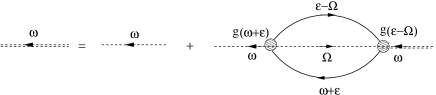
Figure 1: (Color online) Diagram for the pseudofermion self energy.

Through similar bosonization and refermionization procedures as in equilibrium lehur1 ; lehur2 ; Markus ; matveev , the above model is maped onto an equivalent anisotropic Kondo model in an effective magnetic field $h$ with the effective left $L$ and right $R$ Fermi-liquid leadschung . The effective Kondo model takes the form:

$${H}_{K} = \sum_{k,\gamma=L,R,\sigma=\uparrow,\downarrow}[\epsilon_{k}-\mu_{\gamma}]c_{k\gamma\sigma}^{\dagger}c_{k\gamma\sigma}$$ (2)

$$+ (J_{\perp}^{1}s_{LR}^{+}S^{-}+J_{\perp}^{2}s_{RL}^{+}S^{-}+h.c.)$$

$$+ \sum_{\gamma=L,R}J_{z}s_{\gamma\gamma}^{z}S^{z}+hS_{z},$$

where $c_{kL(R)\sigma}^{\dagger}$ is the electron operator of the effective lead $L(R)$, with spin $\sigma$. Here, the spin operators are related to the electron operators on the dot by: $S^{+}=d^{\dagger}$, $S^{-}=d$, and $S^{z}=d^{\dagger}d-1/2=n_{d}-1/2$ where $n_{d}=d^{\dagger}d$ describes the charge occupancy of the level. The spin operators for electrons in the effective leads are $s_{\gamma\beta}^{\pm}=\sum_{\alpha,\delta,k,k^{\prime}}1/2c_{k\gamma\alpha}^{\dagger}\mathbf{\sigma}_{\alpha\delta}^{\pm}c_{k^{\prime}\beta\delta}$, the transverse and longitudinal Kondo couplings are given by $J_{\perp}^{1(2)}\propto{t_{1(2)}}$ and $J_{z}\propto 1/2(1-{1}/\sqrt{2\alpha^{\ast}})$ respectively, and the effective bias voltage is $\mu_{\gamma}=\pm\frac{V}{2}\sqrt{1/(2\alpha^{\ast})}$, where $1/\alpha^{\ast}=1+\alpha$. Note that $\mu_{\gamma}\rightarrow\pm V/2$ near the transition ($\alpha^{\ast}\rightarrow 1/2$ or $\alpha\rightarrow 1$) where the above mapping is exact. The spin operator of the quantum dot in the effective Kondo model $\vec{S}$ can also be expressed in terms of spinful pseudofermion operator $f_{\sigma}$: $S_{i=x,y,z}=f^{\dagger}_{\alpha}\sigma_{i=x,y,z}^{\alpha\beta}f_{\beta}$. In the Kondo limit where only the singly occupied fermion states are physically relevant, a projection onto the singly occupied states is necessary in the pseudofermion representationRosch ; chung . This can be achieved by introducing the Lagrange multiplier $\lambda$ so that $Q=\sum_{\gamma}f^{\dagger}_{\gamma}f_{\gamma}=1$paaske ; latha . In equilibrium, the above anisotropic Kondo model exhibits the Kosterlitz-Thouless (KT) transition from a delocalized phase with a finite conductance $G\approx\frac{1}{2\pi\hbar}$ ($e=\hbar=1$) for $J_{\perp}+J_{z}>0$ to a localized phase for $J_{\perp}+J_{z}\leq 0$ with vanishing conductance. The distinct profile in nonequilibrium transport near the localized-delocalized KT transition has been addressed in Ref. chung . Below we will turn our attention to the dynamical charge susceptibility of the quantum dot close to the transition.

Nonequilibrium FRG formalism. The non-equilibrium perturbative FRG approach is based on the generalization of the perturbative RG approach studied in Ref. Rosch for the nonequilibrium Kondo model. Following Ref. woelfleFRG , the frequency dependent RG scaling equations for the effective Kondo couplings in the Keldysh formulation are given byRosch :

$$\frac{\partial g_{z}(\omega)}{\partial\ln D} = -\sum_{\beta=-1,1}\left[g_{\perp}\left(\frac{\beta V}{2}\right)\right]^{2}\Theta_{\omega+\frac{\beta V}{2}}$$

$$\frac{\partial g_{\perp}(\omega)}{\partial\ln D} = -\sum_{\beta=-1,1}g_{\perp}\left(\frac{\beta V}{2}\right)g_{z}\left(\frac{\beta V}{2}\right)\Theta_{\omega+\frac{\beta V}{2}},$$ (3)

where $g_{\perp}(\omega)=N(0)J_{\perp}^{1}=N(0)J_{\perp\sigma}^{2}$, $g_{z}(\omega)=N(0)J_{z}$ are dimensionless frequency-dependent Kondo couplings with $N(0)$ being density of states per spin of the conduction electrons (we assume symmetric hopping $t_{1}=t_{2}=t$). Here, $\Theta_{\omega}=\Theta(D-|\omega+\mathit{i}\Gamma(\omega)|)$ (with $D<D_{0}$ being the running cutoff) comes from the leading logarithmic corrections for the Kondo vertex function originated from the product of the Keldysh component of the lead electron Green function $G_{\alpha}^{K}(\omega)$ with the real part of the retarded or advanced dressed pseudo fermion propagator $Re(\tilde{G}_{f}^{R/A})$woelfleFRG :

$$G_{\alpha}^{K}(\omega) = -2\pi{\it i}\tanh(\frac{\omega-\mu_{\alpha}}{2T})N_{0}\Theta(D_{0}-|\omega|)$$

$$\tilde{G}_{f\sigma}^{R}(\omega) = \frac{1}{\omega-\Sigma_{\sigma}^{R}(\omega)}=[\tilde{G}_{f\sigma}^{A}(\omega)]^{\ast},$$ (4)

where $\Sigma_{\sigma}^{R}(\omega)=Re(\Sigma_{\sigma}^{R}(\omega))+\frac{{\it i}}{2}\Gamma_{\sigma}(\omega)$ is the impurity self-energy (defined below) with the imaginary part being the dynamical decoherence rate $\Gamma_{\sigma}(\omega)$, and $N_{0}=\frac{1}{2D_{0}}$. At $T=0$, the above correction can be approximated by the $\Theta$-function in the RG equations shown above. Also, the dynamical decoherence (dephasing) rate $\Gamma_{\sigma}(\omega)$ at finite bias which serves as a cutoff to the RG flow of $g_{\perp,z}(\omega)$Rosch , and it is determined self-consistently along with the RG equations for the Kondo couplings. Note that in general $\Gamma_{\sigma}(\omega)$ depends on the impurity spin $\sigma$; however, in the absence of the magnetic field as we consider here, we have the spin symmetry and hence: $\Gamma_{\uparrow}(\omega)=\Gamma_{\downarrow}(\omega)=\Gamma(\omega)$. We can obtain $\Gamma(\omega)$ by the imaginary part of the pseudofermion self energy via second-order renormalized perturbation theory (see Fig. 1):

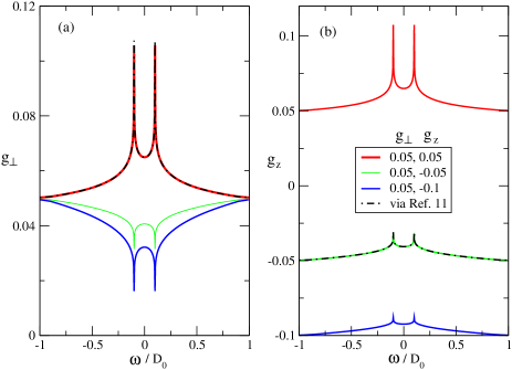
Figure 2: Frequency dependent Kondo couplings of a dissipative resonant level model at zero temperature for (a). $g_{\perp}(\omega)$ and (b). $g_{z}(\omega)$ across the localized-delocalized transition for different bare Kondo couplings via the FRG approach (solid lines) and the approach in Ref. chung (dot-dashed lines). We have set $V=0.2D_{0}$ where $D_{0}=1$ for all the figures.

$$\Gamma_{\sigma}(\omega) = Im(\Sigma_{\sigma}(\omega))={\it i}(\Sigma_{\sigma}^{R}-\Sigma_{\sigma}^{A})$$

$${\it i}\Sigma_{\sigma}^{R(A)}(\omega) = \sum_{\alpha,\beta=L,R}\frac{\theta_{\sigma\sigma^{\prime}}}{16}\int\frac{d\epsilon}{2\pi}g_{\alpha\beta}(\omega+\epsilon)$$

$$\chi_{cf,\sigma^{\prime}}^{<(>),\alpha\beta}(\epsilon)G_{\beta}^{>(<)}(\epsilon+\omega)$$

where $\sigma=\uparrow,\downarrow$, $\theta_{\sigma\sigma^{\prime}}$ is the tensor associated with the product of the Pauli matricesRosch :

$$\theta_{\gamma\gamma^{\prime}}=\frac{1}{2}\sum_{\sigma,\sigma^{\prime}}\tau^{i}_{\sigma\sigma^{\prime}}\tau^{i}_{\gamma\gamma^{\prime}}\tau^{j}_{\sigma^{\prime}\sigma}\tau^{j}_{\gamma^{\prime}\gamma}=\delta_{\gamma\gamma^{\prime}}+2\tau^{1}_{\gamma^{\prime}\gamma}$$ (6)

, and $\chi_{cf,\sigma}^{<(>),\alpha\beta}$ reads:

$$\chi_{cf,\sigma}^{<(>),\alpha\beta}(\epsilon)=\int\frac{d\Omega}{2\pi}g_{\beta\alpha}(\epsilon-\Omega)(\hat{G}_{\alpha\sigma}(\epsilon+\Omega)\hat{G}_{f\sigma}(\Omega))^{<(>)},$$ (7)

where $\hat{G}$ is the Green’s function in $2\times 2$ Keldysh space, and its lesser and greater Green’s function are related to its retarded, advanced, and Keldysh components by:

$$G^{<} = (G^{K}-G^{R}+G^{A})/2$$

$$G^{>} = (G^{K}+G^{R}-G^{A})/2$$ (8)

Specifically, the lesser and greater components of Green’s function of the conduction electron in the leads and of the quantum dot (impurity) are given by (in the absence of magnetic field):

$$G_{L/R}^{<}(\epsilon) = {\it i}A_{c}(\epsilon)f_{\epsilon-\mu_{L/R}}$$

$$G_{L/R}^{>}(\epsilon) = {\it i}A_{c}(\epsilon)(1-f_{\epsilon-\mu_{L/R}})$$

$$G_{f\sigma}^{<}(\epsilon) = 2\pi{\it i}\delta(\epsilon)n_{f\sigma}(\epsilon)$$

$$G_{f\sigma}^{>}(\epsilon) = 2\pi{\it i}\delta(\epsilon)(n_{f\sigma}(\epsilon)-1)$$ (9)

where $A_{c}(\epsilon)=2\pi N_{0}^{2}\Theta(D_{0}-\epsilon)$ is the density of states of the leads, $n_{f\sigma}(\epsilon)=f^{\dagger}_{\sigma}f_{\sigma}$ is the occupation number of the pseudofermion which obeys $n_{f\uparrow}+n_{f\downarrow}=1$, $n_{f\sigma}(\epsilon\rightarrow 0)=1/2$ in the delocalized phase and $n_{f\uparrow}(\epsilon\rightarrow 0)\rightarrow 0$, $n_{f\downarrow}(\epsilon\rightarrow 0)\rightarrow 1$ in the localized phasechung ; latha . Here, the pseudofermion occupation number $n_{f\sigma}$ and the occupation number on the dot $n_{d}$ are related via $<n_{f\uparrow}-n_{f\downarrow}>=<n_{d}>-1/2$. Also, $f_{\omega-\mu_{L/R}}$ is the Fermi function of the $L/R$ lead given by $f_{\omega-\mu_{L/R}}=1/(1+e^{(\omega-\mu_{L/R})/k_{B}T}))$. We have therefore:

$$\chi_{cf,\sigma}^{<,\alpha\beta}(\epsilon) = 2\pi{\it i}g_{\beta\alpha}(\epsilon)A_{c}(\epsilon)(1-n_{f\sigma}(\epsilon))f_{\epsilon-\mu_{\alpha}}$$

$$\chi_{cf,\sigma}^{>,\alpha\beta}(\epsilon) = 2\pi{\it i}g_{\beta\alpha}(\epsilon)A_{c}(\epsilon)n_{f\sigma}(\epsilon)(1-f_{\epsilon-\mu_{\alpha}})$$ (10)

$$\Gamma(\omega)=\frac{3}{4\pi} \int{d\epsilon} g_{\perp}(\epsilon+\omega)g_{\perp}(\epsilon)[f_{\epsilon-\mu_{L}}(1-f_{\epsilon+\omega-\mu_{R}})]$$ (11)

$$+ g_{z}(\epsilon+\omega)g_{z}(\epsilon)[f_{\epsilon-\mu_{L}}(1-f_{\epsilon+\omega-\mu_{L}})]$$

$$+ (L\rightarrow R)$$

The FRG approach here is accomplished by self-consistently solving the RG scaling equation Eq. 3 subject to Eq. LABEL:Gamma-omega and Eq. 11. The solutions at zero temperature for $g_{\perp}(\omega)$ and $g_{\sigma,z}(\omega)$ across the transition are shown in Fig. 2chung . Note that our FRG approach is somewhat different from that in Ref. woelfleFRG : We do not formulate and solve for the RG scaling equation for the impurity self energy $\Sigma_{\sigma}(\omega)$ as shown in Ref. woelfleFRG ; instead, we calculate the imaginary part of the impurity self-energy (or the decoherence rate $\Gamma(\omega)$) self-consistently via second-order renormalized perturbation theory. Nevertheless, we have checked in the simple Kondo limit with isotropic couplings that the frequency-dependent renormalized Kondo coupings $g_{\perp,z}(\omega)$ obtained here agree very well with that obtained via an equivalent FRG approach in Ref. woelfleFRG ).

As the system goes from the delocalized to localized phase transition, the features in $g_{\perp}(\omega)$ at $\omega=\pm V/2$ undergoes a crossover from symmetric double peaks to symmetric double dips, while the symmetric two peaks in $g_{z}(\omega=\pm V/2)$ still remain peaks. We find the above results based on the more rigorous FRG approach are in good agreement with the previous heuristic methodchung , which provides us with an independent and consistency check on the previous results. Note, however that from previous approach in Ref. chung and chung2 the decoherence rate was taken approximately as $\Gamma(\omega=0)$; we now generalize this $\Gamma$ by including the frequency dependence. This generalization improves the previous RG formalism and it also provides us with more features in the dynamical quantities across the transition, such as in dynamical charge susceptibility.

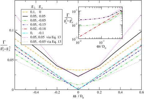
Figure 3: (Color online) $\Gamma(\omega)$ (rescaled to $g_{\perp}^{2}+g_{z}^{2}$ with $g_{\perp,z}$ being the bare Kondo couplings) versus $\omega$ at zero temperature across the delocalized-localized KT transition. Inset: the log-log plot of $\Gamma(\omega)$ versus $\omega$. The bias voltage is fixed at $V=0.2D_{0}$. Here, $D_{0}=1$ for all the figures.

It is worthwhile mentioning that unlike the equilibrium RG at finite temperatures where RG flows are cutoff by temperature $T$, here in nonequilibrium the RG flows will be cutoff by the decoherence rate $\Gamma$, a much lower energy scale than $V$, $\Gamma\ll V$. This explains the dips (peaks) structure in $g_{\perp(z)}(\omega)$ in Fig. 2. In contrast, the equilibrium RG will lead to approximately frequency independent couplings, (or “flat” functions $g_{\perp}(\omega)\approx g_{\perp,z}(\omega=0)$). In the absence of field $h=0$, $g_{\perp,(z)}(\omega)$ show dips (peaks) at $\omega=\pm V/2$. We use the solutions of the frequency-dependent Kondo couplings $g_{\perp,z\sigma}(\omega)$ to compute the dynamical charge susceptibility of the resonance-level near the transition.

Dynamical decoherence rate and charge susceptibility. We have solved for the dynamical decoherence rate $\Gamma(\omega)$ at zero temperature self-consistently along with the RG equations Eq. 3, and the results are shown in Fig. 3. As the general trend, we find $\Gamma(\omega)$ increases with increasing frequency; while it decreases in magnitude at low frequencies $|\omega|<V$ as the system crossovers from the delocalized to the localized phase. is due to In additions, in the delocalized phase, it shows a singular “kink-like” behavior at frequencies $\omega=\pm V$, separating two different behaviors for $|\omega|>V$ and $|\omega|<V$. The curves of $\Gamma(\omega)$ for $|\omega|<V$ are closer to the linear behavior than those for $|\omega|>V$. As the system moves to the localized phase, $\Gamma(\omega)$ for both $|\omega|<V$ and $|\omega|>V$ gradually changes its slopes or curvatures and finally merges into a single linear behavior deep in the localized phase (see Fig. 3).

To understand the above qualitative features, it proves useful to simplify the zero temperature dynamical decoherence rate in Eq. 11 to the following form:

$$\Gamma(\omega) = \frac{3}{4\pi}[\int_{-V/2-\omega/2}^{V/2+\omega/2}+\int_{-V/2+\omega/2}^{V/2-\omega/2}]d\epsilon$$

$$\times g_{\perp}(\epsilon-\omega/2)g_{\perp}(\epsilon+\omega/2)$$

$$+ \frac{3}{4\pi}[\int_{V/2-\omega/2}^{V/2+\omega/2}+\int_{-V/2-\omega/2}^{-V/2+\omega/2}]d\epsilon$$

$$\times g_{z}(\epsilon-\omega/2)g_{z}(\epsilon+\omega/2),(|\omega|<V),$$

$$\Gamma(\omega) = \frac{3}{4\pi}[\int_{-V/2-\omega/2}^{V/2+\omega/2}+\int_{V/2-\omega/2}^{-V/2+\omega/2}]d\epsilon$$ (12)

$$\times g_{\perp}(\epsilon-\omega/2)g_{\perp}(\epsilon+\omega/2)$$

$$+ \frac{3}{4\pi}[\int_{V/2-\omega/2}^{V/2+\omega/2}+\int_{-V/2-\omega/2}^{-V/2+\omega/2}]d\epsilon$$

$$\times g_{z}(\epsilon-\omega/2)g_{z}(\epsilon+\omega/2),(|\omega|>V).$$

Figure 4: (Color online) Diagram for the charge susceptibility. The dressed pseudofermion propagator (double dashed line) is calculated via diagram in Fig. 1

In the “flat” (or in the “equilibrium form”) approximation where $g_{\perp,z}(\omega)$ are treated as flat functions $g_{\perp,z}(V,\omega=0)\approx g_{\perp,z}(V=T)$ with $T$ being temperaturechung , Eq. 12 can be simplified as the following linear behaviors:

$$\Gamma^{e}(\omega) = \frac{3}{2\pi}[Vg_{\perp}^{2}(0)+\omega g_{z}^{2}(0)],(|\omega|<V),$$

$$\Gamma^{e}(\omega) = \frac{3}{2\pi}\omega(g_{\perp}^{2}(0)+g_{z}^{2}(0)),(|\omega|>V)$$

As shown in Fig. 3, the above approximated form $\Gamma^{e}(\omega)$ agrees well with $\Gamma(\omega)$ for $|\omega|<V$, but it shows deviation from $\Gamma(\omega)$ for $|\omega|>V$. The approximated form $\Gamma^{e}(\omega)$ exhibits two linear behaviors with different slopes for $|\omega|<V$ and $|\omega|>V$, respectively, leading to a “kink-like” singularity at $\omega=\pm V$. As the system moves from delocalized to localized phase, the ratio $g_{\perp}(0)/g_{z}(0)$ becomes progressively smaller, leading to the suppressions of the two slopes. Finally, as the system is deeply in the localized phase, these two lines merge into a single line since $|g_{\perp}(0)|\ll|g_{z}(0)|$ there. The qualitative behaviors of $\Gamma^{e}(\omega)$ can explain the overall monotonically increasing trend of $\Gamma(\omega)$ with increasing the magnitude of frequency as well as the decreasing trend of $\Gamma(|\omega|<V)$ as the system moves from the delocalized to the localized phase.

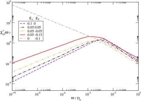
Figure 5: (Color online) $\chi^{"}_{zz}(\omega)$ versus $\omega$ at zero temperature across the localized-delocalized KT transition. The bias voltage is fixed at $V=0.2D_{0}$. Here, $D_{0}=1$ for all the figures.

When the full frequency dependence of $g_{\perp,z}(\omega)$ is considered, we find $\Gamma(\omega)$ deviates from the perfect linear behavior in $\Gamma^{e}(\omega)$ (see Fig. 3). Furthermore, in the delocalized phase, the correction to the linear behavior, $\Gamma(\omega)-\Gamma^{e}(\omega)$ is more noticeable in the large frequency regime ($|\omega|>V$) than in the small frequency regime $|\omega|<V$ (see Fig. 3). This comes as a result of the wider range in energy $\epsilon$ to be integrated over in Eq. 12 for $|\omega|>V$, which accumulates more deviations from the flat approximation due to the dip-peak frequency dependence of $g_{\perp,z}(\omega)$. As the system moves to the localized phase, $\Gamma(|\omega|>V)$ becomes closer to the linear behavior. This is due to the fact that $g_{z}(\omega)$ becomes flatter in the localized phase, giving rise to a more linear behavior for $\Gamma(\omega)$. Meanwhile, based on the solutions for $g_{\perp,z}(\omega)$, we find the correction to the linear behavior as well as the singularities at $\omega=\pm V$ are logarithmic in nature in the isotropic Kondo limit ($g_{\perp}=0.05=g_{z}$) and at the KT transition ($g_{\perp}=0.05=-g_{z}$); while they are power-law in nature for $|g_{\perp}|\neq|g_{z}|$ as $g_{\perp,z}(\omega)$ show logarithmic and power-law properties in these limits, respectivelychung . Note also that for $|\omega|>V$ we find $\Gamma(\omega)<\Gamma^{e}(\omega)$ in the delocalized phase; while the opposite holds in the localized phase. This can be understood as in the delocalized phase we have $|g_{\perp(z)}(\omega)|<|g_{\perp(z)}(0)|$ for the majority of the frequencies (except for $\omega$ very close to $\pm V/2$), leading to a smaller value of $\Gamma(\omega)$ compared to $\Gamma^{e}(\omega)$; while the opposite is true in the localized phase. We have checked numerically that $\Gamma(\omega=0)$ obtained here indeed reproduces the frequency independent decoherence rate $\Gamma$ obtained in Ref. chung .

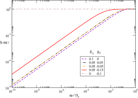
Figure 6: (Color online) $h(\omega)$ versus $\omega$ at zero temperature across the localized-delocalized KT transition. The bias voltage is fixed at $V=0.2D_{0}$. Here, $D_{0}=1$ for all the figures.

The effect of the dynamical decoherence rate can be measured experimentally via dynamical charge susceptibility $\chi_{c}(\omega)$: $Im(\chi_{c}(\omega))\propto\lim_{h\rightarrow 0}dn_{d}(\omega)/dh$ with $h\propto(N-1/2)$ being the effective magnetic field measuring the deviations of $N$ electrons on the dot from the charge degeneracy point. Here, $\chi_{c}(\omega)$ is the Fourier-transformed charge susceptibility defined as:

$$\chi_{c}(t)\equiv{\it i}\theta(t)<[(n_{d}(t)-1/2),(n_{d}(0)-1/2)]>$$ (14)

Experimentally, the dynamical charge susceptibility can be measured by the capacitance lineshape in an AC field near the charge degeneracy point via the high sensitivity charge sensor in the Single Electron Transistor (SET) connected to the dotberman . The decoherence rate $\Gamma(\omega=0)$ here corresponds to the broadening of the resonance peak in the imaginary part of $\chi_{c}(\omega)$. We have calculated $\chi_{c}(\omega)$ at zero temperature based on the renormalized second-order perturbation theory (see the diagram in Fig. 4). From the mapping mentioned above, the dynamical charge susceptibility $\chi_{c}(\omega)$ is related to the $z-$component of the effective “spin-spin” correlation function $\chi_{zz}$ in the effective Kondo model through:

$$\chi_{c}(t) \equiv {-\it i}\theta(t)<[(n_{d}(t)-1/2),(n_{d}(0)-1/2)]>$$

$$\equiv \chi_{zz}(t),$$

$$\chi_{zz}(t) \equiv -{\it i}\theta(t)<[S_{z}(t),S_{z}(0)]>$$ (15)

Taking the Fourier transform of $\chi_{zz}(t)$ and evaluating the diagram in Fig. 4, the imaginary part of $\chi_{zz}(\omega)$, $\chi_{zz}^{"}(\omega)=Im(\chi_{zz}(\omega))$ is given by:

$$\chi_{zz}{"}(\omega) = \int\frac{d\epsilon}{2\pi}\sum_{\sigma=\uparrow,\downarrow}[\bar{G}_{f,\sigma}^{<}(\omega+\epsilon)\bar{G}_{f,\sigma}^{>}(\epsilon)$$ (16)

$$- \bar{G}_{f,\sigma}^{>}(\omega+\epsilon)\bar{G}_{f,\sigma}^{<}(\epsilon)],$$

where $\bar{G}^{>(<))}$ denote the greater (lesser) components of the dressed pseudofermion Green’s functions:

$$\bar{G}_{f\sigma}^{<}(\omega) = {2\pi\it i}n_{f\sigma}(\omega)\bar{A}_{f\sigma}(\omega)$$

$$\bar{G}_{f\sigma}^{>}(\omega) = {2\pi\it i}(n_{f\sigma}(\omega)-1)\bar{A}_{f\sigma}(\omega)$$

$$\bar{A}_{f\sigma}(\omega) = Im[\frac{1}{\omega+\Sigma_{f\sigma}(\omega)+{\it i}\eta}],$$ (17)

where $n_{f\sigma}(\omega)$ is the nonequilibrium occupation number determined self-consistently by the quantum Boltzmann equationpaaske :

$$n_{\sigma}(\omega)=(1-\Sigma^{>}_{\sigma}(\omega)/\Sigma^{<}_{\sigma}(\omega))^{-1}$$ (18)

where $\Sigma^{>(<)}_{\sigma}(\omega)$ are defined in Ref. latha . The resulting expression for $\chi_{zz}(\omega)$ at $T=0$ is given by:

$$\chi_{zz}^{"}(\omega)=\frac{\Gamma(\omega)}{\omega^{2}+\Gamma^{2}(\omega)}\times(1-2n_{f\uparrow}(\omega))$$ (19)

where $n_{f\uparrow}(\omega)$ is given bypaaske :

$$n_{f\uparrow}(\omega) \approx \frac{1}{2}\frac{g_{\perp}^{2}(0)(V-\omega)}{2g_{z}^{2}(0)\omega+g_{\perp}^{2}(0)(V+\omega)},(0<\omega<V)$$

$$n_{f\uparrow}(\omega) \approx \frac{1}{2}\frac{g_{\perp}^{2}(0)(V-\omega-2g^{2}_{z}\omega)}{g_{\perp}^{2}(0)(V+\omega)},(-V<\omega<0).$$

Note that we have neglected the vertex correction in the calculation for $\chi_{zz}(\omega)$ as it gives only a sub-leading correction to Eq. 19.

As shown in Fig. 7, in the delocalized phase, $\chi_{zz}(\omega\rightarrow 0)\propto\omega\rightarrow 0$; while $\chi_{zz}(\omega\rightarrow 0)\rightarrow 1/\omega$ in the localized phase. Hence, as the system crossovers from delocalized to localized phase $\chi_{zz}^{"}(\omega)$ shows a dip-to-peak crossover for small $\omega$. This behavior can be understood as follows. In the delocalized (Kondo screened) phase, the effective local “spin” get Kondo screened in the low energy scale; therefore, the spin susceptibility should vanish. On the other hand, in the localized (ferromagnetic) phase, the unscreened free “spin” gives rise to the Curie-law susceptibility $\chi_{zz}^{"}(\omega)\propto 1/\omega$ at low energies. Meanwhile, in the delocalized phase, we find a a “kink-like” singular behavior in $\chi_{zz}^{"}(\omega)$ at $\omega=V$, coming from the singular behaviors of both $\Gamma(\omega=V)$ (see Eq. 3) and the factor $1-2n_{f\uparrow}$ in $\chi^{"}_{zz}(\omega=V)$ (see Eq. 19 and discussions below). However, this singularity gets smeared out as the system crossovers to the localized phase. We have checked that our results for $\chi_{zz}^{"}(\omega)$ in the isotropic Kondo limit agrees qualitatively well with those in Ref. schoeller and Ref. kehrein2 . For $\omega\gg V$, we find Curie-like susceptibility $\chi_{zz}^{"}(\omega)\propto 1/\omega$ in both localized and delocalized phases, followed Eq. 19 and Eq. LABEL:GammaEQ.

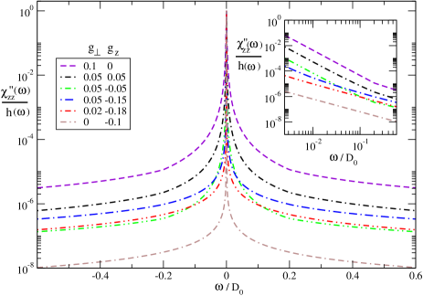
Figure 7: (Color online) $\chi^{"}_{zz}(\omega)/h(\omega)$ (normalized to $1$) versus $\omega$ at zero temperature across the localized-delocalized KT transition. Here, $h(\omega)$ is defined in the text. Inset: the log-log plot of $\chi^{{}^{\prime}}_{zz}(\omega)$ (normalized to $1$) versus $\omega$. The bias voltage is fixed at $V=0.2D_{0}$. Here, $D_{0}=1$ for all the figures.

We can furthermore link our results to the equilibrium and nonequilibrium fluctuation-dissipation theoremschoeller ; coleman ; kehrein ; kehrein2 ; mitra . It is useful to define the dynamical fluctuation-dissipation ratio $h(\omega)$:

$$h(\omega)=\frac{\chi_{zz}^{"}(\omega)}{S_{zz}(\omega)},$$ (21)

where $S_{zz}(\omega)$ is the Fourier-transformed longitudinal spin-spin correlation function with its real-time form given by:

$$S_{zz}(t)=\frac{1}{2}<\{S_{z}(t),S_{z}(0)\}>.$$ (22)

The dynamical spin-spin correlation function $S(\omega)$ is given by:

$$S(\omega) = \int\frac{d\epsilon}{2\pi}\sum_{\alpha=\uparrow,\downarrow}[\bar{G}_{f,\alpha}^{<}(\omega+\epsilon)\bar{G}_{f,\alpha}^{>}(\epsilon)$$ (23)

$$+ \bar{G}_{f,\alpha}^{>}(\omega+\epsilon)\bar{G}_{f,\alpha}^{<}(\epsilon)],$$

Carrying out similar calculations as in $\chi_{zz}^{"}(\omega)$, we find the fluctuation-dissipation ratio $h(\omega)$ reads:

$$h(\omega)=1-2n_{f\uparrow}(\omega),$$ (24)

where $n_{f\uparrow}(\omega)$ is defined in Eq. LABEL:nf. In equilibrium, the ratio $h(\omega)\equiv h^{0}(\omega)$ respects the fluctuation-dissipation theoremcoleman ; schoeller ; kehrein ; kehrein2 , given by $h^{0}(\omega)=1-2n_{f}^{0}(\omega)=\tanh(\beta\omega/2)$ where $n_{f}^{0}(\omega)=\frac{1}{e^{\beta\omega}+1}$ is the Fermi function for pseudofermion in equilibrium. At $T=0$ ($\beta\rightarrow\infty$), we have $h^{0}(\omega>0)=1$, the signature of the equilibrium fluctuation-dissipation theorem at $T=0$. In nonequilibrium and at $T=0$, however, we find in general a deviation of $h(\omega)$ in the delocalized phase from the equilibrium fluctuation-dissipation theorem: $h(\omega)<1$ for $\omega<V$schoeller ; coleman , and $h(\omega\rightarrow 0)\propto\omega\rightarrow 0$ (see Fig. 6 and Eq. 24, Eq. LABEL:nf); while we recover the equilibrium fluctuation-dissipation theorem $h(\omega)=1$ for $|\omega|>V$, in agreement with the results in found in Ref. schoeller . However, that as the system moves to the deep localized phase, the above deviation gets smaller and finally we recover the equilibrium fluctuation-dissipation theorem for all frequencies: $h(\omega)=1$ for all $|\omega|<D_{0}$ (see Fig. 6). To more clearly observe the singular property of $\chi^{"}(|\omega|=V)$, we also plot the normalized Lorentzian form $\Gamma(0)\chi^{"}(\omega)/h(\omega)=\Gamma(\omega)\Gamma(0)/(\omega^{2}+\Gamma^{2}(\omega))$ (see Fig. 7). As the system moves from the delocalized to the localized phase, the width of the Lorentzian peak gets narrower and the singularity at $\omega=V$ gradually disappears.

.3 Conclusions

In conclusion, we have calculated the zero temperature nonequilibrium dynamical decoherence rate and charge susceptibility of a dissipative quantum dot. The system corresponds to a nonequilibrium anisotropic Kondo model. We generalized previous RG approach based on Anderson’s poor man’s scaling approach and renormalized perturbation theory to a more rigorous functional RG (FRG) approach. Within the FRG approach, as the systems crossover from the delocalized to the localized phase, we find a crossover in dynamical charge susceptibility from a dip to a peak structure for $|\omega|<V$. Meanwhile, we find a smeared-out of the singular behavior in charge susceptibility at $\omega=\pm V$ in the above crossover. We also show the deviation of the equilibrium fluctuation-dissipation theorem for small frequencies $\omega<V$; while the theorem is respected when the system is in the extremely localized phase. The above signatures can be used to identify experimentally the above localized-delocalized quantum phase transition out of equilibrium in nano-systems associated with the Kondo effect.

- (1) S. Sachdev, Quantum Phase Transitions, Cambridge University Press (2000).
- (2) S. L. Sondhi, S. M. Girvin, J. P. Carini, and D. Shahar, Rev. Mod. Phys. 69, 315 (1987).
- (3) K. Le Hur, Phys. Rev. Lett. 92, 196804 (2004); M.-R. Li, K. Le Hur, and W. Hofstetter, Phys. Rev. Lett. 95, 086406 (2005).
- (4) K. Le Hur and M.-R. Li, Phys. Rev. B 72, 073305 (2005).
- (5) P. Cedraschi and M. Büttiker, Annals of Physics (NY) 289, 1 (2001).
- (6) A. Furusaki and K. A. Matveev, Phys. Rev. Lett. 88, 226404 (2002).
- (7) L. Borda, G. Zarand, and D. Goldhaber-Gordon, cond-mat/0602019.
- (8) G. Zarand, C.H. Chung, P. Simon, and M. Vojta, Phys. Rev. Lett. 97, 166802 (2006).
- (9) G. Refael, E. Demler, Y. Oreg, and D. S. Fisher, Phys. Rev. B 75, 014522 (2007).
- (10) J. Gilmore and R. McKenzie, J. Phys. C. 11, 2965 (1999).
- (11) C.H. Chung, K. Le Hur, M. Vojta and P. Wölfle, Phys. Rev. Lett 102, 216803 (2009).
- (12) C.H. Chung, K.V.P. Latha, K. Le Hur, M. Vojta and P. Wölfle, arXiv:1002.1757.
- (13) C.H. Chung and K.V.P. Latha, arXiv:1002.4038 (to appear in Phys. Rev. B).
- (14) A. Rosch, J. Paaske, J. Kroha, and P. Wölfle, Phys. Rev. Lett. 90, 076804 (2003); A. Rosch, J. Paaske, J. Kroha, P. Wöffle, J. Phys. Soc. Jpn. 74, 118 (2005).
- (15) J. Paaske, A. Rosch, J. Kroha, and P. Wöffle, Phys. Rev. B 70, 155301 (2004); J. Paaske, A. Rosch, P. Wöffle, Phys. Rev. B 69, 155330 (2004).
- (16) H. Schmidt and P. Wëlfle, Ann. Phys. (Berlin) 19, No. 1-2, 60-74 (2010).
- (17) Severin G. Jakobs, Mikhail Pletyukhov, and Herbert Schoeller, Phys. Rev. B 81, 195109 (2010).
- (18) Andreas Hackl, David Roosen, Stefan Kehrein, Walter Hofstetter, Phys. Rev. Lett. 102, 196601 (2009); P. Fritsch, S. Kehrein, Phys. Rev. B 81, 035113 (2010).
- (19) P. Fritsch and S. Kehrein, Ann. Phys. 324, 1105 (2009).
- (20) W. Mao, P. Coleman, C. Hooley, and D. Langreth, Phys. Rev. Lett. 91, 207203 (2003).
- (21) A. Mitra, A. J. Millis, Phys. Rev. B 72, 121102 (R) (2005).
- (22) D. Berman, N. B. Zhitenev, R. C. Ashoori, H. I. Smith, and M. R. Melloch, J. Vac. Sci. Technol. B 15, 2844 (1997); D. Berman, N. B. Zhitenev and R. C. Ashoori, and M. Shayegan, Phys. Rev. Lett. 82, 161 (1999); K. W. Lehnert, B. A. Turek, K. Bladh, L. F. Spietz, D. Gunnarsson, P. Delsing, and R. J. Schoelkopf, Phys. Rev. Lett. 91, 106801 (2003).
- (23) E. Kim, cond-mat/0106575 (unpublished).
- (24) M. Fabrizio and A. O. Gogolin, Phys. Rev. B 51, 17827 (1995).
- (25) Serge Florens, Pascal Simon, Sabine Andergassen, and Denis Feinberg, Phys. Rev. B 75, 155321 (2007).