Accuracy guarantees for -recovery ††thanks: Research of the second author was supported by the Office of Naval Research grant # N000140811104 and the NSF grant DMS-0914785.
Abstract
We discuss two new methods of recovery of sparse signals from noisy observation based on -minimization. While they are closely related to the well-known techniques such as Lasso and Dantzig Selector, these estimators come with efficiently verifiable guaranties of performance. By optimizing these bounds with respect to the method parameters we are able to construct the estimators which possess better statistical properties than the commonly used ones.
We link our performance estimations to the well known results of Compressive Sensing and justify our proposed approach with an oracle inequality which links the properties of the recovery algorithms and the best estimation performance when the signal support is known. We also show how the estimates can be computed using the Non-Euclidean Basis Pursuit algorithm.
Key words
: sparse recovery, linear estimation, oracle inequalities, nonparametric estimation by convex optimization
AMS Subject Classification
: 62G08, 90C25
1 Introduction
Recently several methods of estimation and selection which refer to the -minimization received much attention in the statistical literature. For instance, Lasso estimator, which is the -penalized least-squares method is probably the most studied (a theoretical analysis of the Lasso estimator is provided in, e.g., [2, 3, 4, 19, 20, 21, 17, 18], see also the references cited therein). Another, closely related to the Lasso, statistical estimator is the Dantzig Selector [7, 2, 16, 17]. To be more precise, let us consider the estimation problem as follows. Assume that an observation
| (1) |
is available, where is an unknown signal and is a known sensing matrix. We suppose that is a Gaussian disturbance with (i.e., , where are independent normal r.v.’s with zero mean and unit variance), and is a known deterministic noise level. Our focus is on the recovery of unknown signal .
The Dantzig Selector estimator of the signal is defined as follows [7]:
where is the algorithm’s parameter. Since is obtained as a solution of an linear program, it is very attractive by its low computational cost. Accuracy bounds for this estimator are readily available. For instance, a well known result about this estimator (cf. [7, Theorem 1.1]) is that if then
with probability if the signal is -sparse, i.e. has at most non-vanishing components, and the sensing matrix with unit columns possesses the Restricted Isometry Property with parameters and . 111Recall that , called also uniform uncertainty principle, means that for any with at most nonzero entries, This property essentially requires that every set of columns of with cardinality less than approximately behaves like an orthonormal system. Further, in this case one has , where is a moderate absolute constant. This result is quite impressive, in part due to the fact (see, e.g. [5, 6]) that there exist random matrices, with , which possess the RIP with probability close to , close to zero and the value of as large as . Similar performance guarantees are known for Lasso recovery
with properly chosen penalty parameter . The available accuracy bounds for Lasso and Dantzig Selector rely upon the Restricted Isometry Property or less restrictive assumptions about the sensing matrix, such as Restricted Eigenvalue [2] or Compatibility [3] conditions (a complete overview of those and several other assumptions with description of how they relate to each other is provided in [19]). However, these assumptions cannot be verified efficiently. The latter implies that there is currently no way to provide any guaranties (e.g., confidence sets) of the performance of the proposed procedures. A notable exception from this rule is the Mutual Incoherence assumption (see, e.g. [10, 11, 12] and [21] for the case of, respectively, deterministic and random observation noise) which can be used to compute the accuracy bounds for recovery algorithms: a matrix with columns of unit -norm and mutual incoherence possesses with .222 The mutual incoherence of a sensing matrix is computed according to Obviously, the mutual incoherence can be easily computed even for large matrices. Unfortunately, the latter relation implies that should be very small to certify the possibility of accurate -recovery of non-trivial sparse signals, so that performance guarantees based on mutual incoherence are very conservative. This “theoretical observation” is supported by numerical experiments – the practical guarantees which may be obtained using the mutual incoherence are generally quite poor even for the problems with nice theoretical properties (cf. [14, 15]).
Recently the authors have proposed a new approach for efficient computing of upper and lower bounds on the “level of goodness” of a sensing matrix , i.e. the maximal such that the -recovery of all signals with no more than non-vanishing components is accurate in the case where the measurement noise vanishes (see [14]). In the present paper we aim to use the related verifiable sufficient conditions of “goodness” of a sensing matrix to provide efficiently computable bounds for the error of recovery procedures in the case when the observations are affected by random noise.
The main body of the paper is organized as follows:
-
1.
We start with Section 2.1 where we formulate the sparse recovery problem and introduce our core assumption – a verifiable condition linking matrix and a contrast matrix . In Sections 2.2, 2.3 we present two recovery routines with contrast matrices:
-
•
regular recovery:
-
•
penalized recovery:
( is our guess for the number of nonzero entries in the true signal, is the penalty parameter)
along with their performance guarantees under condition with , that is, explicit upper bounds on the confidence levels of the recovery errors . The novelty here is that our bounds are of the form
(2) (with hidden factors in independent of ), and are valid in the entire range of values of . Note that similar error bounds for Dantzig Selector and Lasso are only known for , whatever be the assumptions on “essentially nonsquare” matrix .
-
•
-
2.
Our interest in condition stems from the fact that this condition, in contrast to the majority of the known sufficient conditions for the validity of -based sparse recovery (e.g., Restricted Isometry/Eigenvalue/Compatibility), is efficiently verifiable. Moreover, it turns out that one can efficiently optimize the error bounds of the associated with this verifiable condition regular/penalized recovery routines over the contrast matrix . The related issues are considered in Section 3. In Section 4 we provide some additional justification of the condition , in particular, by linking it with the Mutual Incoherence and Restricted Isometry properties. This, in particular, implies that the condition with, say, associated with randomly selected matrices is feasible, with probability approaching 1 as grow, for as large as . We also establish limits of performance of the condition, specifically, show that unless is nearly square, with can be feasible only when , meaning that the tractability of the condition has a heavy price: when designing and validating minimization based sparse recovery routines, this condition can be useful only in a severely restricted range of the sparsity parameter .
-
3.
In Section 5 we show that the condition is the strongest (and seemingly the only verifiable one) in a natural family of conditions linking a sensing and a contrast matrix; here is the number of nonzeros in the sparse signal to be recovered . We demonstrate that when a contrast matrix satisfies with , the associated regular and penalized recoveries admit error bounds similar to (2), but now in the restricted range of values of . We demonstrate also that feasibility of with implies instructive (although slightly worse than those in (2)) error bounds for the Dantzig Selector and Lasso recovering routines.
-
4.
In Section 6, we present numerical results on comparison of regular/penalized recovery with the Dantzig Selector and Lasso algorithms. The conclusion suggested by these preliminary numerical results is that when the former procedures are applicable (i.e., when the techniques of Section 3 allow to build a “not too large” contrast matrix satisfying the condition with, say, ), our procedures outperform significantly the Dantzig Selector and work exactly as well as the Lasso algorithm with “ideal” (unrealistic in actual applications) choice of the regularization parameter333With “theoretically optimal,” rather than “ideal,” choice of the regularization parameter in Lasso, this algorithm is essentially worse than our algorithms utilizing the contrast matrix..
-
5.
In the concluding Section 7 we present a “Non-Euclidean Matching Pursuit algorithm” (similar to the one presented in [15]) with the same performance characteristics as those of regular/penalized recoveries; this algorithm, however, does not require optimization and can be considered as a computationally cheap alternative to recoveries, especially in the case when one needs to process a series of recovery problems with common sensing matrix.
All proofs are placed in the Appendix.
2 Accuracy bounds for -Recovery Routines
2.1 Problem statement
Notation.
For a vector and we denote the vector obtained from by setting to all but the largest in magnitude entries of . Ties, if any, could be resolved arbitrarily; for the sake of definiteness assume that among entries of equal magnitudes, those with smaller indexes have priority (e.g., with one has ). stands for the usual -norm of (so that ). We say that a vector is -sparse if it has at most nonzero entries. Finally, for a set we denote by its complement ; given , we denote by the vector obtained from by zeroing the entries with indices outside of , so that .
Given a norm on and a matrix , we set .
The problem.
We consider an observation
| (3) |
where is an unknown signal and is the sensing matrix. We suppose that is a Gaussian disturbance, where (i.e., with independent normal random variables with zero mean and unit variance), being known, and is a nuisance parameter known to belong to a given uncertainty set which we will suppose to be convex, compact and symmetric w.r.t. the origin. Our goal is to recover from , provided that is “nearly -sparse.” Specifically, we consider the sets
of signals which admit -sparse approximation of -accuracy . Given , , and a confidence level , , we quantify a recovery routine — a Borel function — by its worst-case, over , confidence interval, taken w.r.t. -norm of the error. Specifically, we define the risks of a recovery routine as
Equivalently: if and only if there exists a set of “good” realizations of with such that whenever , one has for all and all .
Norm .
Given and let us denote
| (4) |
Since is convex, closed and symmetric with respect to the origin, is a norm. Let be the norm on conjugate to :
Conditions and .
Let . Given , consider the following condition on a matrix :
: for all and one has
(5)
Now let be a positive integer and . Given , we say that a matrix satisfies condition 444The reason for this cumbersome, at the first glance, notation will become clear later, in Section 5., if
| (6) |
The conditions we have introduced are closely related to each other:
Lemma 1
If satisfies , then satisfies , and “nearly vice versa:” given satisfying , one can build efficiently a matrix satisfying with (i.e., ) and such that the columns of are convex combinations of the columns of and , so that for every norm on .
2.2 Regular Recovery
In this section we discuss the properties of the regular -recovery given by:
| (7) |
where is as in (3), , , are some vectors in and , . We refer to the matrix as to the contrast matrix underlying the recovering procedure.
The starting point of our developments is the following
Proposition 1
Given an sensing matrix , noise intensity , uncertainty set and a tolerance , let the matrix from (7) satisfy the condition for some , and let in (7) satisfy the relation
| (8) |
where is given by (4). Then there exists a set , , of ”good” realizations of such that
(i) Whenever , for every , every and every subset such that
| (9) |
the regular -recovery given by (7) satisfies:
where and
(ii) In particular, when setting
| (11) |
and assuming , for every , and it holds
(iii) Finally, assuming , for every , and one has
| (14) |
The following result is an immediate corollary of Proposition 1:
Lemma 2
The next statement is similar to the cases of in Proposition 1 and Lemma 2; the difference is that now we assume that satisfies , which, by Lemma 1, is a weaker requirement on than to satisfy with .
Proposition 2
Given an sensing matrix , noise intensity , uncertainty set and a tolerance , let the matrix from (7) satisfy the condition for some , and let in (7) satisfy the relation (8). Then there exists a set , , of ”good” realizations of such that whenever , for every and every one has
| (19) |
In particular,
| (20) |
2.3 Penalized Recovery
Now consider the penalized -recovery as follows:
| (21) |
where is as in (3), and an integer , a positive , and a matrix are parameters of the construction.
Proposition 3
Given an sensing matrix , an integer , a matrix and positive reals , , satisfying the condition , and a , assume that
| (22) |
and
| (23) |
Further, let , , and let
| (24) |
Consider the penalized recovery associated with . There exists a set , , of ”good” realizations of such that
(ii) When and , one has for every , and :
| (26) |
whence for every and :
| (27) |
The next statement is in the same relation to Proposition 3 as Proposition 2 is to Proposition 1 and Lemma 2.
Proposition 4
Given an sensing matrix , noise intensity , uncertainty set and a tolerance , let the matrix from (21) satisfy the condition for some , and let . Then there exists a set , , of ”good” realizations of such that whenever , for every and every one has
| (30) |
In particular,
| (31) |
Note that under the premise of Proposition 2, the smallest possible values of are the quantities , which results in ; with this choice of , the risk bound for the regular recovery, as given by the right hand side in (20), coincides within factor 2 with the risk bound for the penalized recovery with as given by (31); both bounds assume that satisfies with and imply that
| (32) |
When , the latter bound admits a quite transparent interpretation: everything is as if we were observing the sum of an unknown -dimensional signal and an observation error of the uniform norm .
3 Efficient construction of the contrast matrix
In what follows, we fix , the “environment parameters” and the “level of sparsity” of signals we intend to recover, and are interested in building the contrast matrix resulting in as small as possible error bound (32). All we need to this end is to answer the following question (where we should specify the norm as ):
(?) Let be a norm on , and be a positive integer. What is the domain of pairs such that and there exists matrix satisfying the condition and the relation ? How to find such an , provided it exists?
Invoking Lemma 1, we can reformulate this question as follows:
(??) Let and be as in (?). Given , how to find vectors , , satisfying
for every , or to detect correctly that no such collection of vectors exists?
Indeed, by Lemma 1, if satisfies and , then there exists such that satisfy for all and , so that satisfy for all as well. Vice versa, if satisfy , , then the matrix clearly satisfies , and .
The answer to (??) is given by the following
Lemma 3
Given , , and a positive integer , let . For every , the following three properties are equivalent to each other:
-
(i)
There exists satisfying ;
-
(ii)
The optimal value in the optimization problem
where is -th standard basic orth in , is ;
-
(iii)
One has
(33) where is the norm on conjugate to .
Whenever one (and then – all) of these properties take place, problem is solvable, and its optimal solution satisfies .
3.1 Optimal contrasts for regular and penalized recoveries
As an immediate consequence of Lemma 3, we get the following description of the domain associated with the norm :
| (34) |
where in is specified as . Note that the second equality in is given by Linear Programming duality. Indeed, by , is the smallest for which all problems , , are feasible, and thus, by Lemma 3, if and only if and .
Note that the quantity depends solely of , while depends on , as on parameters, but is independent of .
The outlined results suggest the following scheme of building the contrast matrix :
-
•
we compute by solving Linear Programming problems in (34.); if , then does not contain points with , so that our recovery routines are not applicable (or, at least, we cannot justify them theoretically);
-
•
when , the set is nonempty, and its Pareto frontier (the set of pairs such that is possible if and only if ) is the curve , . We choose a “working point” on this curve, that is, a point and compute by solving the convex optimization programs , , with specified as . is nothing but the maximum, over , of the optimal values of these problems, and the optimal solutions to the problems induce the matrix which satisfies and has . By reasoning which led us to (??),
that is, is the best for our purposes contrast matrices satisfying . With this contrast matrix, the error bound (32) for regular/penalized recoveries (in the former, , in the latter, ) read
(35)
The outlined strategy does not explain how to choose . This issue could be resolved, e.g., as follows. We choose an upper bound on the sensitivity of the risk (35) to , i.e., to the -deviation of a signal to be recovered from the set of -sparse signals. This sensitivity is proportional to , so that an upper bound on the sensitivity translates into an upper bound on . We can now choose by minimizing the remaining term in the risk bound over , which amounts to solving the optimization problem
Observing that is, by its origin, a convex function, we can solve the resulting problem efficiently by bisection in . A step of this bisection requires solving a univariate convex feasibility problem with efficiently computable constraint and thus is easy, at least for moderate values of .
4 Range of feasibility of condition
We address the crucial question of what can be said about the magnitude of the quantity , see (34) and the risk bound (35). One way to answer it is just to compute the (efficiently computable!) quantity for a desired value of . Yet it is natural to know theoretical upper bounds on in some “reference” situations. Below, we provide three results of this type.
At this point, it makes sense to express in the notation that depends, as on parameters, on the sensing matrix and the “environment parameters” , so that in this section we write instead of .
4.1 Bounding via mutual incoherence
Recall that for an sensing matrix with no zero columns, its mutual incoherence is defined as
Compressed Sensing literature contains numerous mutual-incoherence-related results (see, e.g., [10, 11, 12] and references therein). To the best of our knowledge, all these results state that if is a positive integer and is a sensing matrix such that , then -based sparse recovery is well suited for recovering -sparse signals (e.g., recovers them exactly when there is no observation noise, admit explicit error bounds when there is noise and/or the signal is only nearly -sparse, etc.). To the best of our knowledge, all these results, up to the values of absolute constant factors in error bounds, are covered by the risk bounds (35) combined with the following immediate observation:
Observation 1
Whenever is an matrix with no zero columns and is a positive integer, the matrix satisfies the condition .
Verification is immediate: the diagonal entries in the matrix are equal to , while the magnitudes of the off-diagonal entries in do not exceed . Therefore
Observe that the Euclidean norms of the columns in do not exceed , whence , where . In the notation from Section 3, our observations can be summarized as follows:
Corollary 1
For every matrix with no zero columns, one has and . In particular,
It should be added that as grow in such a way that , realizations of “typical” random matrices (e.g., those with independent entries or with independent entries taking values ) with overwhelming probability satisfy and for all . By Corollary 1, it follows that for these the condition with, say, can be satisfied for as large as merely by the choice , which ensures that ; in particular, in the indicated range of values of one has .
4.2 The case of satisfying the Restricted Isometry Property
Proposition 5
Let satisfy with some and with . Then there exists matrix which, for every positive integer , satisfies the condition , with
| (36) |
and is such that . In particular,
| (37) |
4.3 Oracle inequality
Here we assume that possesses the following property (where is a positive integer and ):
: For every and every -element subset of there exists a routine for recovering from a noisy observation
of unknown signal , known to be supported on such that for every such signal and every one has
We intend to demonstrate that in this situation for all in certain range (which extends as grows and decreases) the uniform error of the regular and the penalized recoveries associated with properly selected contrast matrix is, with probability , “close” to . The precise statement is as follows:
Proposition 6
Given and the “environment parameters” , , , assume that satisfies the condition with certain . Then for every integer from the range
| (38) |
(here is the standard matrix norm, the largest singular value) there exists a contrast matrix satisfying the condition and such that , so that in the outlined range of values of one has , and the associated with error bound (35) for regular/penalized recovery is
| (39) |
Proposition 6 justifies to some extent, our approach; it says that if there exists a routine which recovers -sparse signals with a priori known sparsity pattern within certain accuracy (measured component-wise), then our recovering routines exhibit “close” performance without any knowledge of the sparsity pattern, albeit in a smaller range of values of the sparsity parameter.
4.4 Condition : limits of performance
Recall that when recovering -sparse signals, the condition helps only when . Unfortunately, with these , the condition is feasible in a severely restricted range of values of . Specifically, from [15, Proposition 5.1] and Lemma 1 it immediately follows that
(*) If is not “nearly square,” that is, if , then the condition with cannot be satisfied when is “large”, namely, when .
Note that from the discussion at the end of section 4.1 we know that the “ limit of performance” of the condition stated in (*) is “nearly sharp:” – when , the condition associated with a typical randomly generated sensing matrix is feasible and can be satisfies with a contrast matrix with quite moderate .
(*) says that unless is nearly square, the condition can validate sparse recovery only in a severely restricted range of values of the sparsity parameter. This is in sharp contrast with unverifiable sufficient conditions for “goodness” of recovery, like RIP: it is well known that when grow, realizations of “typical” random matrices, like those mentioned at the end of Section 4.1, with overwhelming probability possess with as large as . As a result, “unverifiable” sufficient conditions, like RIP, can justify the validity of recovery routines in a much wider (and in fact – the widest possible) range of values of the sparsity parameter than the “fully computationally tractable” condition . This being said, note that this comparison is not completely fair. Indeed, aside of its tractability, the condition with ensures the error bounds (35) in the entire range of values of , which perhaps is not the case with conditions like RIP. Specifically, consider the “no nuisance” case , and let satisfy for certain . It is well known (see, e.g., the next section) that in this case the Dantzig Selector recovery ensures for every and every -sparse signal that
with probability . However, we are not aware of similar bounds (under whatever conditions) for “large” and . For comparison: in the case in question, for “small” , namely, , we have (by Proposition 5), whence for regular and penalized recoveries with appropriately chosen contrast matrix (which can be built efficiently!) one has for all -sparse
with probability (see (35)). We wonder whether a similar (perhaps, with extra logarithmic factors) bound can be obtained for large (e.g., ) for a whatever recovery routine and a whatever essentially nonsquare (say, ) sensing matrix with columns of Euclidean length .
5 Extensions
We are about to demonstrate that the pivot element of the preceding sections — the condition — is the strongest (and seemingly the only verifiable one) in a natural parametric series of conditions on a contrast matrix ; every one of these conditions validates the regular and the penalized recoveries associated with in certain restricted range of values of in the error bounds (35).
5.1 Conditions
Let us fix an sensing matrix . Given a positive integer , a and a real , let us say that an contrast matrix satisfies condition , if
| (40) |
where and , as always, is the vector obtained from by zeroing all but the largest in magnitude entries. Observe that
-
•
What used to be denoted before, is exactly what is called now;
-
•
If satisfies , satisfies for all (since for -sparse vector we have ).
Less immediate observations are as follows:
-
•
Let be an matrix and let be a positive integer. We say that is -good if for all -sparse the -recovery
is exact in the case of noiseless observation . It turns out that feasibility of with is intimately related to -goodness of :
Lemma 4
is -good if and only if there exist and satisfying .
-
•
The Restricted Isometry Property implies feasibility of with small :
Lemma 5
Let satisfy with . Then the matrix satisfies the condition with .
5.2 Regular and penalized recoveries with contrast matrices satisfying
Our immediate goal is to obtain the following extension of the main results of Section 2, specifically, Propositions 2, 4:
Proposition 7
Assume we are given an sensing matrix , an integer , , a contrast matrix , and such that satisfies the condition . Denote , where the norm is defined in (4), and . Let also noise intensity , uncertainty set and tolerance be given.
(i) Consider the regular recovery (7) with the contrast matrix and the parameters satisfying the relations
and let . Then
| (41) |
(ii) Consider the penalized recovery (21) with the contrast matrix and . Then
| (42) |
5.3 Error bounds for Lasso and Dantzig Selector under condition
We are about to demonstrate that the feasibility of condition with implies some consequences for the performance of Lasso and Dantzig Selector when recovering -sparse signals in norms, . This might look strange at the first glance, since neither Lasso nor Dantzig Selector use contrast matrices. The surprise, however, is eliminated by the following observation:
(!) Let satisfy and let be the maximum of the Euclidean norms of columns in . Then
(43)
The fact that a condition like (43) with plays a crucial role in the performance analysis of Lasso and Dantzig Selector is neither surprising nor too novel. For example, the standard error bounds for the latter algorithms under the RIP assumption are in fact based on the validity of (43) with for (see Lemma 5). Another example is given by the Restricted Eigenvalue [2] and the Compatibility conditions [3, 19]. Specifically, the Restricted Eigenvalue condition ( is positive integer, , states that
whence whenever , so that
| (44) |
Further, the Compatibility condition of [19] is nothing but (44) with . We see that both Restricted Eigenvalue and Compatibility conditions imply (43) with , and certain .
We are about to present a simple result on the performance of Lasso and Dantzig Selector algorithms in the case when satisfies the condition (43). The result is as follows:
Proposition 8
Let matrix satisfy (43) with and some , and let . Let also the “environment parameters” , be given, and let there be no nuisance: .
(i) Consider the Dantzig Selector recovery
where
| (45) |
Then
| (46) |
(ii) Consider the Lasso recovery
and let satisfy the relation
where is given by (45). Then
| (47) |
In particular, with
| (48) |
one has
| (49) |
Discussion.
Let us compare the error bounds given by Propositions 7, 8. Assume that there is no nuisance () and is such that the condition is satisfied by certain matrix , the maximum of Euclidean norms of the columns of being . Assuming that the penalized recovery uses , and the regular recovery uses ), the associated risk bounds as given by Proposition 7 become
| (50) |
Note that these bounds admit a transparent interpretation: in the range an -sparse signal is recovered as if we were identifying correctly its support and estimating the entries with the uniform error .
Now, as we have already explained, the existence of a matrix satisfying with columns in being of Euclidean lengths implies validity of (43) with . Assuming that in Dantzig Selector one uses , and that in Lasso is chosen according to (48), the error bounds for Dantzig Selector and Lasso as given by Proposition 8 become
| (51) |
Observe that (look what happens with (43) when is the -th basic orth). We see that the bounds (51) are worse than the bounds (50), primarily due to the presence of the factor in the first bracketed term in (51). At this point it is unclear whether this drawback is an artifact caused by poor analysis of the Dantzig Selector and Lasso algorithms or it indeed “reflects reality.” Some related numerical results presented in Section 6.1 suggest that the latter option could be the actual one.
Moreover, consider an example of the recovery problem with a matrix with unit columns and singular values and . It can be easily seen that if is aligned with the second right singular vector of (corresponding to the singular value ) the error of the Dantzig Selector may be as large as , while the error of “-conscious” recovery will be up to the logarithmic factor in (indeed, choosing results in ). This toy example suggests that the extra factor in the bound (51), at least for Dantzig Selector, is not only due to our clumsy analysis.
This being said, it should be stressed that the comparison of regularized/penalised recoveries with Dantzig Selector and Lasso based solely on above the error bounds is somehow biased against Dantzig Selector and Lasso. Indeed, in order for regular/penalized recoveries to enjoy their “good” error bounds, we should specify the required contrast matrix, which is not the case for Lasso and Dantzig Selector: the bounds (51) require only existence of such a matrix555And even less than that, since feasibility of is just a sufficient condition for the validity of (43), the condition which indeed underlies Proposition 8.. Besides this, there is at least one case where error bounds for Dantzig Selector are as good as (50), specifically, the case when possesses, say, . Indeed, in this case, by Lemma 5, the matrix satisfies , meaning that Dantzig Selector with properly chosen is nothing but the regular recovery with contrast matrix and as such obeys the bounds (50) with .
It is time to point out that the above discussion is somehow scholastic: when and is nontrivial, we do not know how to verify efficiently the fact that the condition is satisfied by a given , not speaking about efficient synthesis of satisfying this condition. One should not think that these tractability issues concern only our algorithms which need a good contrast matrix. In fact, all conditions which allow to validate Dantzig Selector and Lasso beyond the scope of the “fully tractable” condition are, to the best of our knowledge, unverifiable – they cannot be checked efficiently, and thus we never can be sure that Lasso and Dantzig Selector (or any other known computationally efficient technique for sparse recovery) indeed work well for a given sensing matrix. As we have seen in Section 3, the situation improves dramatically when passing from unverifiable conditions , , to the efficiently verifiable condition , although in a severely restricted range of values of .
6 Numerical examples
We present here a small simulation study.
6.1 Regular/penalized recovery vs. Lasso: no-nuisance case
To illustrate the discussion in Section 5.3, we compare numerical performance of Lasso and penalized recovery in the observation model (1) without nuisance:
where is known. The sensing matrix is specified by selecting at random rows of the Hadamard matrix666The -th Hadamard matrix is given by the recurrence , . It is a matrix with orthogonal rows and all entries equal to ., and “suppressing” the first of the selected rows by multiplying it by 1.e-3. The resulting sensing matrix has orthogonal rows; 119 of its 120 singular values are equal to , and the remaining singular value is .
We have processed as explained in Section 3 (a reader is referred to this section for the description of entities involved).777It is worth to mention that when is comprised of (perhaps, scaled) rows of an Hadamard matrix (and in fact, of scaled rows of any other Fourier transform matrix associated with a finite Abelian group) the synthesis described in Section 3 simplifies dramatically due to the fact that all problems turn out to be equivalent to each other, and their optimal solutions are obtained from each other by simple linear transformations. As a result, we can work with a single problem instead of working with of them. We started with computing , which turned out to be 0.0287, meaning that the level of -goodness of is at least 17. In our experiment, we aimed at recovering signals with at most nonzero entries and with no nuisance (). The synthesis of the corresponding “optimal” contrast matrix as outlined in Section 3 results in , . Note that we are in the case of , and in this case the optimal is independent of the values of and .
We compare the penalized -recovery with the contrast matrix and with the Lasso recovery on randomly generated signals with 10 nonzero entries. We consider two choices of the penalty in Lasso: the “theoretically optimal” choice (48) and the “ideal” choice, where we scanned the “fine grid” , of values of and selected the value for which the Lasso recovery was at the smallest -distance from the true signal. The confidence parameter in (48) was set to .
The results of a typical experiment are presented in Table 1. We see that as compared to the penalized recovery, the accuracy of Lasso with the theoretically optimal choice of the penalty is nearly 10 times worse. With the “ideal” (unrealistic!) choice of penalty, Lasso is never better than the penalized recovery, and for the smallest value of is nearly 4 times worse than the latter routine.
| Recovery | |||||
| Penalized | N/A | 2.1e-4 | 6.5e-5 | 3.8e-5 | |
| Lasso | 1.e-4 | 3.74e-3∗ | 2.1e-4 | 5.2e-4 | 3.9e-5 |
| Lasso | 4.01e-2† | 1.6e-3 | 5.2e-4 | 2.0e-4 | |
| Penalized | N/A | 2.2e-5 | 6.0e-6 | 2.7e-6 | |
| Lasso | 1.e-5 | 4.78e-4∗ | 3.1e-5 | 8.1e-6 | 3.4e-6 |
| Lasso | 4.01e-3† | 1.8e-4 | 5.8e-5 | 2.1e-5 | |
| Penalized | N/A | 2.1e-6 | 6.2e-7 | 2.5e-7 | |
| Lasso | 1.e-6 | 1.10e-4∗ | 8.8e-6 | 1.6e-6 | 5.9e-7 |
| Lasso | 4.01e-4† | 1.8e-5 | 5.4e-6 | 1.9e-6 | |
6.2 The nuisance case
In the second experiment we study the behavior of recovery procedures in the situation when an “input nuisance” is present:
where is an unknown sparse signal, with known , is known and is standard normal ; in terms of (3), and . We compare the performance of the regular and penalized recoveries to that of the Lasso and Dantzig Selector algorithms. To handle the nuisance, the latter methods were modified as follows: instead of the standard Lasso estimator we use the estimator
where the penalization coefficient is chosen according to [2, Theorem 4.1]; in turn, the Dantzig Selector is substituted by
with , where are the columns of and is given (in what follows ).
We present below the simulation results for two setups with :
-
1.
Gaussian setup: a sensing matrix with independent entries is generated, then its columns are normalized. The nuisance set is as follows:
where is a known parameter; in other words, we observe the sum of a sparse signal and “smooth background.”
-
2.
Convolution setup: a sensing matrix is constructed as follows: consider a signal “living” on and supported on the grid . We subject such a signal to discrete time convolution with a kernel supported on the set , and then restrict the result on the grid . This way we obtain a linear mapping . The nuisance set is composed of zero-mean signals on which satisfy
where is the discrete (periodic) homogeneous Laplace operator:
with .
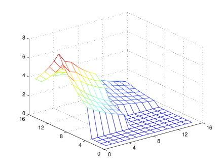
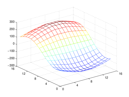
In the simulations we acted as follows: given the sensing matrix , the nuisance set and the values of and , we compute the contrast matrix by choosing a “reasonable” value of and specifying as the matrix satisfying and such that , see Section 3. Then samples of random signal , random nuisance and random perturbation were generated, and the corresponding observations were processed by every one of the algorithms we are comparing888Randomness of the sparse signal is important. Using the techniques of [14], one can verify that in the convolution setup there are signals with only 3 non-vanishing components which cannot be recovered by minimization even in the noiseless case , . In other words, the -goodness characteristic of the corresponding matrix is equal to .. The plots below present the average, over these experiments, and recovery errors. All recovery procedures were using Mosek optimization software [1].
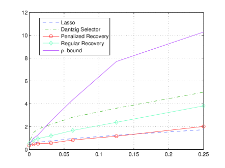
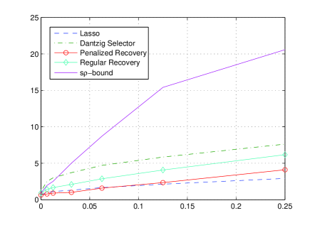
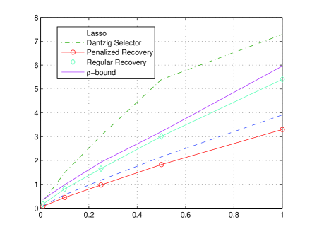
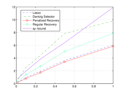
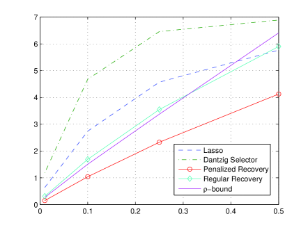
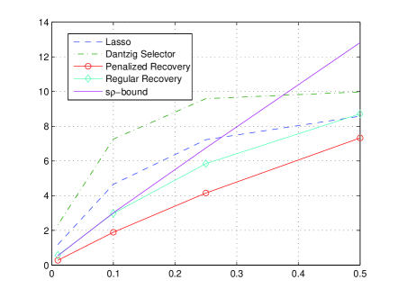
We start with Gaussian setup in which the signal has non-vanishing components, randomly drawn, with . For the penalized and the regular recovery algorithms the contrast matrix was computed using . On Figure 1 we plot the average recovery error as a function of the value of the parameter of the nuisance set , for fixed , and on Figure 2 — as a function of for fixed .
 |
 |
| -error | -error |
 |
 |
| -error | -error |
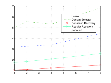
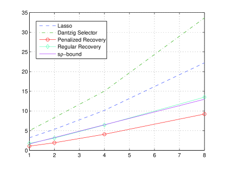
In the next experiment we fix the “environmental parameters” , and vary the number of nonzero entries in the signal (of norm ). On Figure 3 we present the recovery error as a function of .
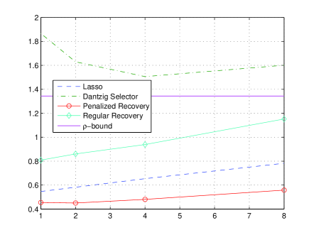 |
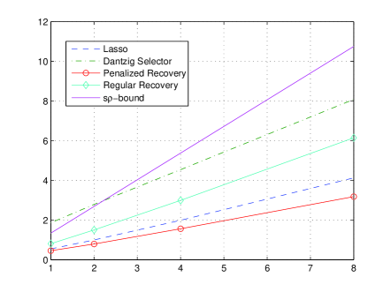 |
| -error | -error |
We run the same simulations in the convolution setup. The contrast matrix for the penalized and the regular recoveries is computed using . On Figure 4 we plot the average recovery error as a function of the “size” of the nuisance set for fixed , on Figure 5 — as a function of for fixed , and on Figure 6 — as a function of .
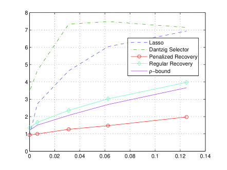 |
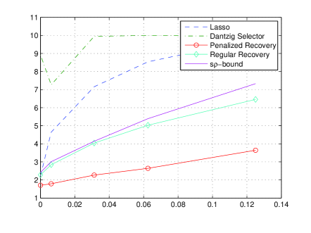 |
| -error | -error |
 |
 |
| -error | -error |
 |
 |
| -error | -error |
We observe quite different behavior of the recovery procedures in our two setups. In the Gaussian setup the nuisance signal does not mask the true signal , and the performance of the Lasso and Dantzig Selector is quite good in this case. The situation changes dramatically in the convolution setup, where the performance of the Lasso and Dantzig Selector degrades rapidly when the parameter of the nuisance set increases.999The error plot for these estimators on Figure 4 flatters for higher values of simply because they always underestimate the signal, and the error of recovery is always less than the corresponding norm of the signal. The conclusion suggested by the outlined numerical results is that the penalized recovery, while sometimes losing slightly to Lasso, in some of the experiments outperforms significantly all other algorithms we are comparing.
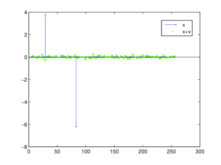 |
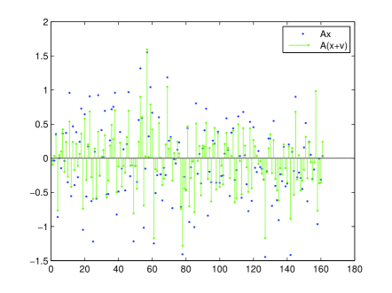 |
| signal and nuisance | image and |
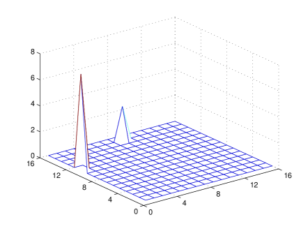 |
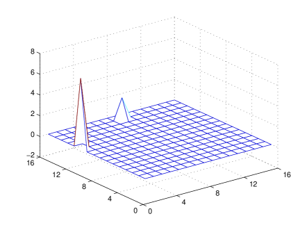 |
| signal | recovery |
 |
 |
| signal image | observation |
7 Non-Euclidean matching pursuit algorithm
The Matching Pursuit algorithm for sparse recovery is motivated by the desire to provide a reduced complexity alternative to the algorithms using -minimization. Several implementations of Matching Pursuit has been proposed in the Compressive Sensing literature (see, e.g., [11, 10, 12]). They are based on successive Euclidean projections of the signal and the corresponding performance results rely upon the bounds on mutual incoherence parameter of the sensing matrix. We are about to show how the construction of Section 3 can be used to design a specific version of the Matching Pursuit algorithm which we refer to as Non-Euclidean Matching Pursuit (NEMP) algorithm. The NEMP algorithm can be an interesting option if the -recovery is to be used repeatedly on the observations obtained with the same sensing matrix ; the numerical complexity of the pursuit algorithm for a given matrix may only be a fraction of that of the recovery, especially when used on high-dimensional data.
Suppose that we have in our disposal such that the condition is feasible; invoking Lemma 3, in this case we can find efficiently a contrast matrix such that
| (52) |
where, as always, with given by (4).
Consider a signal such that , where, as usual, is the vector obtained from by replacing all but the largest in magnitude entries in with zeros, and let be an observation as in (3).
Suppose that , and let be given. Consider the following iterative procedure:
Algorithm 1
-
1.
Initialization: Set ,
-
2.
Step , : Given and , compute
-
(a)
and vector with the entries
(here ).
-
(b)
Set and
(53) and loop to step .
-
(a)
-
3.
The approximate solution found after iterations is .
Proposition 9
Assume that and an is given. Then there exists a set , , of ”good” realizations of such that whenever , for every satisfying and every , the approximate solution and the value after the -th step of Algorithm 1 satisfy
Note that if then also and Proposition 9 holds true. Furthermore, by (53) the sequence converges exponentially fast to the limit :
Along with the second inequality of this implies the bounds:
and, since for ,
The bottom line here is as follows:
Corollary 2
To put this result in proper perspective, note that the mutual incoherence based condition
underlying typical convergence results for the Matching Pursuit algorithms as applied to recovery of -sparse signals (see, e.g. [11, 10, 12]) definitely is sufficient for convergence of the NEMP algorithm with , see Section 4.1. It follows that the scope of NEMP is at least as wide as that of “theoretically valid” Matching Pursuit algorithms known from the literature; in the situation in question Corollary 2 recovers some results from [10, 11, 12].
References
-
[1]
Andersen, E. D., Andersen, K. D. The MOSEK optimization tools manual. Version 5.0
http://www.mosek.com/fileadmin/products/50/tools/doc/html/tools/index.html - [2] Bickel, P., Ritov, Y. and Tsybakov, A. B. Simultaneous analysis of Lasso and Dantzig selector. Ann. Statist., 37, 1705-1732 (2009).
- [3] Bühlmann, P., van de Geer, S. On the conditions used to prove oracle results for the Lasso Electron. J. Statist., 3, 1360-1392 (2009).
- [4] Bunea, F., Tsybakov, A.B. and Wegkamp, M.H. Sparsity oracle inequalities for the Lasso. Electron. J. Stat., 1, 169-194 (2007).
- [5] Candès, E., Romberg, J., Tao T. Robust uncertainty principles: exact signal reconstruction from highly incomplete frequency information. IEEE Trans. Inform. Theory, 52 489-509 (2006).
- [6] Candès, E., Romberg, J., Tao T. Stable signal recovery from incomplete and inaccurate measurements. Comm. Pure Appl. Math., 59 1207-1223 (2006).
- [7] Candès, E. and Tao, T. The Dantzig selector: statistical estimation when is much larger than . Ann. Statist., 35, 2313-2351 (2007).
- [8] Candès, E. J. The restricted isometry property and its implications for compressed sensing. Comptes Rendus de l’Acad. des Sci., Serie I, 346, 589 592 (2008).
- [9] Donoho, D., Statistical estimation and optimal recovery. The Annals of Statistics 22, 1, 238-270 (1995).
- [10] Donoho, D., Elad, M. Optimally sparse representation in general (non-orthogonal) dictionaries via minimization. Proc. Natl. Acad. Sci. USA, 100, 2197-2202 (2003).
- [11] Elad, E., Bruckstein, A.M. A generalized uncertainty principle and sparse representation in pairs of bases. IEEE Trans. Inform. Theory, 48, 2558-2567 (2002).
- [12] Gribonval, R., Nielsen, R. Sparse representations in unions of bases. IEEE Trans. Inform. Theory, 49, 3320-3325 (2003).
- [13] Juditsky, A. B., Nemirovski A.S. Nonparametric estimation by convex programming. Ann. Statist., 37, 5a, 2278-2300 (2009).
- [14] Juditsky, A., Nemirovski, A. On verifiable sufficient conditions for sparse signal recovery via minimization. Mathematical Programming, 127:1, 57-88 (2011).
- [15] Juditsky, A., Kilinç Karzan, F., Nemirovski, A. Verifiable conditions of -recovery of sparse signals with sign restrictions. Mathematical Programming, 127:1, 89-122 (2011).
- [16] Koltchinskii, V. The Dantzig selector and sparsity oracle inequalities. Bernoulli, 15 799-828 (2009).
- [17] Lounici, K. Sup-norm convergence rate and sign concentration property of Lasso and Dantzig estimators. Electronic Journal of Statistics, 2, 90-102 (2008).
- [18] Meinshausen, N. and Yu, B. Lasso-type recovery of sparse representations for high-dimensional data. Annals of Statistics, 37, 246-270 (2009).
- [19] van de Geer, S. The deterministic Lasso. In JSM proceedings, American Statistical Association (2007) (see also http://stat.ethz.ch/research/research_reports/2007/140).
- [20] Zhang, C.-H., Huang, J. The sparsity and bias of the Lasso selection in highdimensional linear regression. Ann. Statist., 36, 1567-1594 (2008).
- [21] Zhang, T. Some sharp performance bounds for least squares regression with regularization. Ann. Statist., 37, 2109-2144 (2009).
Appendix A Proofs
A.1 Proofs for section 2
A.1.1 Proof or Lemma 1
The first claim is evident. Now let satisfy , and let , . Then for every and every with we have
or, which is the same,
By von Neumann lemma, this is the same as
and the outer clearly is achieved, meaning that there exists , , such that with one has
so that for every with one has ; applying the latter inequality to in the role of , we get whenever , whence, of course, for all . We conclude that the matrix satisfies . It remains to note that by construction the columns of are convex combinations of the columns of and , and that building reduces to solving matrix games and thus can be carried out efficiently.
A.1.2 Proof of Proposition 1
Let
so that Let us fix , a set satisfying (9), a signal and a realization of the nuisance, and let be the value of the estimate (7) at the observation . We are about to verify that satisfies (1), which, of course, will complete the proof.
Observe that because of we have
Now, by (8), whence for all , and thus is a feasible solution to the optimization problem in (7) and thus . Setting , we now have , whence . It follows that
| (54) |
Further, . Since is feasible for the optimization problem in (7), we have , and we have already seen that , hence
| (55) |
for all . Applying (5) we now get
where the concluding is given by (54). Taking into account that , we get
Invoking (54) once again, we finally get
and we arrive at (1.).
A.1.3 Proof of Lemma 2
A.1.4 Proof of Proposition 2
The proof is obtained by minor modifications from the one of Proposition 1. Same as in the latter proof, let , where are the columns of , so that Let us fix , , , let , , , . Finally, let be the support of .
Due to , we have
whence, by (8), is a feasible solution to the optimization problem in (7) and thus . The latter, exactly as in the proof of Proposition (1), implies the validity of (54):
| (56) |
Besides this, the same reasoning as in the proof of Proposition 1 results in (55), whence
| (57) |
Applying (6) to , we get
which combines with (56) to imply that
| (58) |
which is nothing but the first relation in (19). Applying to (6) once again, we get
which combines with (58) to imply the second relation in (19). Relation (19) combines with the Moment inequality to imply (20).
A.1.5 Proof of Proposition 3
(i):
Given , , let, same as in the proof of Proposition 1, so that . Let us fix , and a signal , and let us prove that for these data (25) takes place; this clearly will prove (i). Let us set , , , . Let also be the support of .
Observe that by the origin of , we have
| (59) |
and
Combining the resulting inequality with (59), we get
| (60) |
where the concluding is due to combined with (24). Further,
which combines with (60) to imply that
or, which is the same,
| (61) |
By (5), we have
| (62) |
whence and therefore
(ii)–(iii):
A.1.6 Proof of Proposition 4
The proof is obtained by minor modifications from the one of Proposition 1. Same as in the latter proof, let so that .
Let us fix , and a signal . Let us set , , , . Let also be the support of .
A.2 Proofs for sections 3, 4
A.2.1 Proof of Lemma 3
(i)(iii): If satisfies , then for every we have
where the first and the second inequalities are given by and , respectively.
(iii)(ii): Assume that (iii) takes place; then, by homogeneity, for every with , or, which is the same, the optimal value in the
conic problem
is . The problem clearly is strictly feasible and bounded, so that by Conic Duality Theorem the dual problem is solvable with the same optimal value. Now, the dual problem reads
and the fact that it is solvable with the optimal value means that there exist such that , and , whence is a feasible solution to with the value of the objective .
(ii)(i): If is feasible, it clearly is solvable; thus, in the case of (ii) there exists with and . From the latter inequality it follows that for every , so that for all . We see that satisfies , and thus (i) takes place. This reasoning shows also that whenever is feasible with optimal value , it is solvable, and its optimal solution satisfies .
A.2.2 Proof of Proposition 5
Let , , so that what we need to prove is that there exists a matrix satisfying and such that . Invoking Lemma 3, all we need to this end is to show that
| (67) |
Now, we clearly have for all , whence for all . Therefore all we need in order to justify (67) is to prove that
| (68) |
Let . Setting , let vectors be obtained from by the procedure as follows: is obtained by zeroing all but the largest in magnitude entries of ; is obtained by the same procedure from , is obtained by the same procedure from , and so on, until the step where we get . We clearly have , , whence also , , since the vectors are -sparse. Setting and , we have
where the last is given by the following well-known fact: [8]:
(!) If is and are supported on a common set of indices of cardinality and are orthogonal, then .
It follows that
Hence
where the second inequality is due to the fact that by RIP. Thus,
where the concluding inequality is due to and . Recalling that , (68) follows.
A.2.3 Proof of Proposition 6
Proof. We start with analysis of . Let , and let be a subset of of cardinality . Let be the linear space of all vectors from supported on , and let . Assume that we are given a noisy observation of a signal , and that we want to recover from this observation the linear form of the signal. From it follows that there exists a recovering routine such that for every and the probability of recovering error to be is . Assuming and applying the celebrated result of Donoho [9], there exists a linear estimate such that for every and the probability for the error of this estimate to be is . Moreover (cf. Proposition 4.2 of [13]), one can pick such that
where is the matrix obtained from by zeroing columns with indexes not belonging to . Let and , where is the -th basic orth (so that ). Specifying as the vector from such that , and as the vector from such that (the required , clearly exist) and applying to the pair , and to the pair , we get
Hence, denoting by the value of the inverse error function at , we obtain
It follows that as , remains bounded and . Thus, there exists a sequence , of values of such that goes to a limit as , and this limit satisfies the relations
Taking into account that when , we arrive at the following result:
Lemma 6
Under assumption , for every and every -element subset of there exists such that , for all , (here are the columns of ), and
| (69) |
We claim that in this case for all it holds:
| (70) |
Taking this claim for granted, and invoking Lemma 3, we immediately arrive at the desired conclusion. Indeed, given satisfying (38), we have , so that (70) implies that
whence, by Lemma 3, there exists satisfying the condition and such that , which is exactly what Proposition 6 states.
It remains to prove (70). Let us fix , and let be set of indices of the largest in magnitude entries in . Denoting by the complement of in , we have , whence
| (71) |
Let be the index of the largest in magnitude entry of . By Lemma 6 there exists satisfying (69) and such that , for . We have
| (72) |
where the concluding is given by (69). Now,
with the concluding given by (71). The resulting inequality, in view of (72) and the bound given by (69) implies (70).
A.3 Proofs for section 5
A.3.1 Proof of Lemma 4
Recall (cf., e.g., Theorem 2.1 in [14]) that a necessary and sufficient condition for an matrix to be -good is the nullspace property as follows: there exists such that
| (73) |
Assume that this condition is satisfied, and let be a vector with nonzero coordinates, equal to . (73) says that the optimal value in the Linear Programming problem
is at most ; passing to the dual problem, we conclude that there exist and such that and , whence for every it holds
Since the set of the outlined vectors is finite, the quantity is finite, and
meaning that the condition holds true for . Vice versa, the existence of and satisfying clearly implies the validity of (73) with the same and this implies the -goodness of .
A.3.2 Proof of Lemma 5
Let satisfy with ; we want to prove that then the matrix satisfies the condition . Indeed, let . Let vectors be obtained from as follows: is obtained by zeroing all but the largest in magnitude entries of and keeping the latter entries intact, then is obtained by applying the same procedure to , and so on. We stop at step where we get . Observe that , whence also (since is -sparse). We now have
(in the above chain, step is valid due to (since is ) and the statement (!), see the proof of Proposition 5). The concluding inequality in the chain says that satisfies .
A.3.3 Proof of Proposition 7
We present here the proof of (i), which is a straightforward modification of the proof of Proposition 2. The proof of (ii) can be obtained by equally straightforward modification of the proof of Proposition 4.
Thus, suppose we are under the premise of (i), and let be defined exactly as in the proof of Proposition 1, so that and for all , and all . Let us fix , and , let be the set of indices of the largest in magnitude entries in , and let , , , and .
Since and , we have for all , whence is a feasible solution to the optimization problem defining , whence, exactly as in the proof of Proposition 1,
| (74) |
Now, satisfies the condition and thus satisfies the condition . Applying the latter condition, we get
Invoking (74), we conclude that
| (75) |
thus
| (76) |
Next, satisfies , whence . Therefore, we get from (74):
| (77) | |||||
| (78) |
All we need in order to extract (i) from (75) and (78) is to verify that
The desired inequality holds true when (see (75)), thus, invoking the Hölder inequality, all we need is to verify that
| (79) |
When , (79) is implied by (78), so let us assume that . Let be the -st largest of the magnitudes of entries in . By (78) we have , and . Hence, setting , we get
where the concluding inequality is given by (75). Thus, , while by (78). We see that , as required in (79).
A.3.4 Proof of Proposition 8
(i):
Let , so that . Let us fix and , and let , . We have , so that is a feasible solution to the optimization problem specifying and therefore . Denoting by the support of , setting and acting exactly as when deriving (54), we arrive at
| (80) |
Further,
and therefore
| (81) |
On the other hand, by (43) we have
Substituting the above bound into (80), we get
whence by elementary calculations
| (82) |
Invoking (43) and (81), we have
| (83) | |||||
where the last inequality of the chain is due to . Assuming for a moment that and denoting by the -st largest magnitude of entries in , we conclude from the latter inequality that . Hence, when setting we obtain (cf. the verification of (79)) . Invoking (83) one more time we get
The resulting inequality combines with (82) and the Hölder inequality to imply that
| (84) |
Note that the derivation of (84) was carried out under the additional assumption that . This assumption can now be removed: when , (84) is readily given by (82). When , satisfies (43) for and thus – for every value of from , meaning that (84) holds true for every , whence (84) holds true for as well.
(ii):
Same as above, let , so that . Let us fix , , and let be the support of . Let also , , . We have
or, which is the same due to ,
It follows that
where the last is readily given by the fact that for . We conclude that
and therefore
| (85) |
Now, we have
where the concluding inequality is given by (43). Combining the resulting inequality with (85), we get
Combining this inequality with (85), we get the first inequality in the following chain:
and since , we arrive at
| (87) |
Since , the first inequality in (A.3.4) is possible only if
whence
| (88) |
Invoking (43), we get , which combines with (88) and (87) to imply that
| (89) |
Denoting by the -st largest of the magnitudes of entries in , we conclude from (89) that , whence, denoting ,
(we have used (87)), which combines with (89) to imply that
| (90) |
Combining (90), (87) and the Hölder inequality, we get
| (91) |
Plugging in the value of (see (87)) and recalling that (91) takes place whenever with , we arrive at (47).
A.4 Proof of Proposition 9
The proof below follows the lines of the proof of Proposition 7 of [15]. Given , let so that . Let us fix , such that , and . For , by the definition (4) of the norm and because of , we have .
We intend to prove the relations , by induction in . First, let us show that implies . Thus, assume that holds true. Let . By , is supported on the support of . Note that
Then by (52) for any ,
consequently,
| (92) |
so that the segment of the width covers , and the closest to zero point of this interval is
that is, for all . Since the segment covers and is the closest to 0 point in , while the width of is at most , we clearly have
| (95) |
Since is valid, (95.a) implies that
and holds. Further, let be the support of . Relation clearly implies that , and we can write due to (95.b):
Since by (95.b)
we conclude that holds true. The induction step is justified.
It remains to show that holds true. Since is evident, all we need is to justify . Let
and let . Same as above (cf. (92)), we have for all :
Then
Hence
which implies .