$B_{s}\to f_{0}(980)$ decays: Results from light-cone QCD Sum Rules

Abstract

We describe a light-cone QCD sum rule calculation of the $B_{s}\to f_{0}(980)$ transition form factors useful to predict the branching ratios of the rare decays $B_{s}\to f_{0}\ell^{+}\ell^{-}$, $B_{s}\to f_{0}\nu\bar{\nu}$ and of $B_{s}\to J/\psi f_{0}$ decay assuming factorization. We compare this channel to $B_{s}\to J/\psi\phi$ as far as the possibility to determine the $B_{s}$ mixing phase is concerned.

1 Introduction

Rare $B_{s}$ decays induced at loop level in the Standard Model (SM) are sensitive to new physics (NP) effects that may enhance their small branching ratios [1]. Besides, the analysis of the $B_{s}$ unitarity triangle of Cabibbo-Kobayashi-Maskawa (CKM) elements: $V_{us}V_{ub}^{*}+V_{cs}V_{cb}^{*}+V_{ts}V_{tb}^{*}=0$ provides an important test of the SM description of CP violation. One of its angles, $\beta_{s}=Arg\left[-\frac{V_{ts}V^{*}_{tb}}{V_{cs}V^{*}_{cb}}\right]$, is expected to be tiny in the SM: $\beta_{s}\simeq 0.019$ rad. Recently CDF [2] and D0 [3] Collaborations have indicated larger values with sizable uncertainties, although the latest CDF analysis [4] seems to reconcile the SM with data. Hence the precise measurement of $\beta_{s}$ is a priority for forthcoming experiments.
In this paper we describe the light-cone QCD sum rule (LCSR) calculation of the $B_{s}\to f_{0}(980)$  form factors [5], using the results to predict the branching ratios of the decays $B_{s}\to f_{0}\ell^{+}\ell^{-}$, $B_{s}\to f_{0}\nu\bar{\nu}$ in the SM. We also study the mode $B_{s}\to J/\psi f_{0}$ that allows to access $\beta_{s}$ [6].

2 $B_{s}\to f_{0}$ form factors in Light-Cone Sum Rules

The matrix elements involved in $B_{s}\to f_{0}$ transitions can be parameterized in terms of form factors as

$$\langle f_{0}(p_{f_{0}})|\bar{s}\gamma_{\mu}\gamma_{5}b|\overline{B}_{s}(p_{B_{s}})\rangle=$$ (1)

$$-i\Big{\{}F_{1}(q^{2})\Big{[}P_{\mu}-\frac{m_{B_{s}}^{2}-m_{f_{0}}^{2}}{q^{2}}q_{\mu}\Big{]} + F_{0}(q^{2})\frac{m_{B_{s}}^{2}-m_{f_{0}}^{2}}{q^{2}}q_{\mu}\Big{\}},\,\,\,$$

$$\langle{f_{0}}(p_{f_{0}})|\bar{s}\sigma_{\mu\nu}\gamma_{5}q^{\nu}b|\overline{B}_{s}(p_{B_{s}})\rangle=$$

$$-\frac{F_{T}(q^{2})}{m_{B_{s}}+m_{f_{0}}}\Big{[}q^{2}P_{\mu}-(m_{B_{s}}^{2}-m_{f_{0}}^{2})q_{\mu}\Big{]},$$ (2)

where $P=p_{B_{s}}+p_{f_{0}}$ and $q=p_{B_{s}}-p_{f_{0}}$. To compute such form factors using light-cone QCD sum rules (LCSR) [7] we consider the correlation function:

$$\Pi(p_{f_{0}},q)=i\int d^{4}x\,e^{iq\cdot x}\langle{f_{0}}(p_{f_{0}})|{\rm T}\left\{j_{\Gamma_{1}}(x),j_{\Gamma_{2}}(0)\right\}|0\rangle$$ (3)

where $j_{\Gamma_{1}}$ is one of the currents in the definitions (1)-(2) of the form factors: $j_{\Gamma_{1}}=J_{\mu}^{5}=\bar{s}\gamma_{\mu}\gamma_{5}b$ for $F_{1}$ and $F_{0}$, and $j_{\Gamma_{1}}=J_{\mu}^{5T}=\bar{s}\sigma_{\mu\nu}\gamma_{5}q^{\nu}b$ for $F_{T}$. $j_{\Gamma_{2}}=\bar{b}i\gamma_{5}s$ interpolates the $B_{s}$ meson; its matrix element between the vacuum and $B_{s}$ defines the $f_{B_{s}}$ decay constant: $\langle\overline{B}_{s}(p_{B_{s}})|\bar{b}i\gamma_{5}s|0\rangle=\frac{m_{B_{s}}^{2}}{m_{b}+m_{s}}f_{B_{s}}$. The LCSR method consists in evaluating the correlator (3) both at the hadronic level and in QCD. Equating the two representations gives a sum rule suitable to derive the form factors.

The hadronic representation of the correlator in (3) can be written as the contribution of the $\bar{B}_{s}$ plus that of the higher resonances and the continuum of states $h$:

$$\Pi^{\rm H}(p_{f_{0}},q)=\frac{\langle{f_{0}}(p_{f_{0}})|j_{\Gamma_{1}}|\overline{B}_{s}(p_{f_{0}}+q)\rangle\langle\overline{B}_{s}(p_{f_{0}}+q)|j_{\Gamma_{2}}|0\rangle}{m_{B_{s}}^{2}-(p_{f_{0}}+q)^{2}}$$

$$+\int_{s_{0}}^{\infty}ds\frac{\rho^{h}(s,q^{2})}{s-(p_{f_{0}}+q)^{2}},$$ (4)

where higher resonances and the continuum of states are described in terms of the spectral function $\rho^{h}(s,q^{2})$, which contributes starting from a threshold $s_{0}$.

To evaluate the correlator in QCD we write it as

$$\Pi^{\rm QCD}(p_{f_{0}},q)=\frac{1}{\pi}\int_{(m_{b}+m_{s})^{2}}^{\infty}ds\,\frac{{\rm Im}\Pi^{\rm QCD}(s,q^{2})}{s-(p_{f_{0}}+q)^{2}}\,.$$ (5)

Expanding the T-product in (3) on the light-cone, we obtain a series of operators, ordered by increasing twist, the matrix elements of which between the vacuum and the $f_{0}$ are written in terms of $f_{0}$ light-cone distribution amplitues (LCDA). Since the function $\rho^{h}$ in (4) is unknown, we use global quark-hadron duality to identify $\rho^{h}$ with $\rho^{\rm QCD}={1\over\pi}{\rm Im}\Pi^{\rm QCD}$ when integrated above $s_{0}$ [8]:

$$\vspace{-0.8cm}\int_{s_{0}}^{\infty}ds{\rho^{h}(s,q^{2})\over s-(p_{f_{0}}+q)^{2}}=\frac{1}{\pi}\int_{s_{0}}^{\infty}ds\,\frac{{\rm Im}\Pi^{\rm QCD}(s,q^{2})}{s-(p_{f_{0}}+q)^{2}}\,.$$

Using duality, together with the equality $\Pi^{\rm H}(p_{f_{0}},q)=\Pi^{\rm QCD}(p_{f_{0}},q)$, we obtain from Eqs. (4) and (5):

$$\frac{\langle{f_{0}}(p_{f_{0}})|j_{\Gamma_{1}}|\overline{B_{s}}(p_{f_{0}}+q)\rangle\langle\overline{B_{s}}(p_{f_{0}}+q)|j_{\Gamma_{2}}|0\rangle}{m_{B_{s}}^{2}-(p_{f_{0}}+q)^{2}}=$$

$$\frac{1}{\pi}\int_{(m_{b}+m_{s})^{2}}^{s_{0}}ds\,\frac{{\rm Im}\Pi^{\rm QCD}(s,q^{2})}{s-(p_{f_{0}}+q)^{2}}\,\,\ .$$ (6)

We perform a Borel transformation of the two sides in (6), exploiting the result $\displaystyle{{\cal B}\left[{1\over(s+Q^{2})^{n}}\right]={\exp(-s/M^{2})\over(M^{2})^{n}\ (n-1)!}}$ where $Q^{2}=-q^{2}$ and $M^{2}$ is the Borel parameter. This operation improves the convergence of the series in $\Pi^{\rm QCD}$ and for suitable values of $M^{2}$ enhances the contribution of the low lying states to $\Pi^{\rm H}$. Applying it to $\Pi^{\rm H}$ and $\Pi^{\rm QCD}$ we get

$${\langle{f_{0}}(p_{f_{0}})|j_{\Gamma_{1}}|\overline{B}_{s}(p_{B_{s}})\rangle\langle\overline{B}_{s}(p_{B_{s}})|j_{\Gamma_{2}}|0\rangle}{\rm exp}\left[-\frac{m_{B_{s}}^{2}}{M^{2}}\right]=$$

$$\frac{1}{\pi}\int_{(m_{b}+m_{s})^{2}}^{s_{0}}ds\,\,{\rm exp}[-s/M^{2}]\,\,{\rm Im}\Pi^{\rm QCD}(s,q^{2})$$ (7)

($p_{B_{s}}=p_{f_{0}}+q$). From (7) we derive the sum rules for $F_{1}$, $F_{0}$ and $F_{T}$, choosing either $j_{\Gamma_{1}}=J_{\mu}^{5}$ or $j_{\Gamma_{1}}=J_{\mu}^{5T}$.

In the calculation of $\Pi^{\rm QCD}$ we consider $f_{0}$ as a $s\bar{s}$ state modified by some hadronic dressing [9]. Possible $f_{0}-\sigma$ mixing [10] may only affect the overall normalization of the form factors at zero recoil, a systematic uncertainty in our numerical results. We refer to [5] for the definitions of the $f_{0}$ LCDA, for numerical values of the input parameters as well as for the final expressions of the form factors obtained from (7). We fix $s_{0}=(34\pm 2)\,{\rm GeV}^{2}$, which should correspond to the mass squared of the first radial excitation of $B_{s}$. As for the Borel parameter, the form factors for each value of $q^{2}$ depend on it. The result is obtained requiring stability against variations of $M^{2}$.

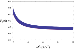
Figure 1: Dependence of $F_{1}^{B_{s}\to f_{0}}(0)$ on the Borel parameter $M^{2}$.

In Fig. 1 we show the dependence of $F_{1}(q^{2}=0)$ on $M^{2}$. We observe stability when $M^{2}>6$ ${\rm GeV}^{2}$, and we fix $M^{2}=(8\pm 2)\,{\rm GeV}^{2}$.

To describe the form factors in the whole kinematically accessible $q^{2}$ region, we use the parameterization $\displaystyle{F_{i}(q^{2})=\frac{F_{i}(0)}{1-a_{i}q^{2}/m_{B_{s}}^{2}+b_{i}(q^{2}/m_{B_{s}}^{2})^{2}}}$, $i\in\{1,0,T\}$. We collect in Table 1 the parameters $F_{i}(0)$, $a_{i}$ and $b_{i}$ obtained fitting the form factors computed numerically. The $q^{2}$ dependence is shown in Fig. 2. The uncertainties in the results are due to the input parameters, $s_{0}$ and $M^{2}$. The parameters $a_{i}$ and $b_{i}$ are close for $F_{1}$ and $F_{T}$. The reason is the following. In the heavy-quark limit and in the large energy (LE) limit of the recoiled meson, the $B_{s}\to f_{0}$ form factors can be related [11] as follows:

$$\frac{m_{B_{s}}}{m_{B_{s}}+m_{f_{0}}}F_{T}(q^{2})=F_{1}(q^{2})=\frac{m_{B_{s}}}{2E}F_{0}(q^{2}),$$ (8)

with $q^{2}=m_{B_{s}}^{2}-2m_{B_{s}}E$ (neglecting $m_{f_{0}}^{2}$). The first equality in (8) predicts the same $q^{2}$ dependence for $F_{1}$ and $F_{T}$ in the LE limit. For the parameters of $F_{0}$, the second equality gives: $a_{0}=-1+a_{1}$, $b_{0}=1-a_{1}+b_{1}$ which, using the results for $a_{1}$ and $b_{1}$, gives $a_{0}^{(LE)}\simeq 0.44\pm 0.1$ and $b_{0}^{(LE)}\simeq 0.15\pm 0.12$. Hence the first relation is respected in our calculation, while not much can be said about the second one due to the uncertainty affecting $b_{0}$.

Table 1: Parameters of the $B_{s}\to f_{0}$ form factors by LCSR.

	$F_{i}(q^{2}=0)$	$a_{i}$	$b_{i}$
$F_{1}$	$0.185\pm 0.029$	$1.44^{+0.13}_{-0.09}$	$0.59^{+0.07}_{-0.05}$
$F_{0}$	$0.185\pm 0.029$	$0.47^{+0.12}_{-0.09}$	$0.01^{+0.08}_{-0.09}$
$F_{T}$	$0.228\pm 0.036$	$1.42^{+0.13}_{-0.10}$	$0.60^{+0.06}_{-0.05}$

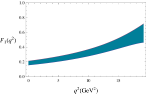
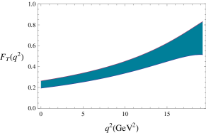
Figure 2: $q^{2}$ dependence of the $B_{s}\to f_{0}$ form factors.

3 Semileptonic $\bar{B}_{s}\to f_{0}\ell^{+}\ell^{-}$ and $\bar{B}_{s}\to f_{0}\nu\bar{\nu}$ decays

$B_{s}$ decays induced by the $b\to s$ transition can constrain new Physics scenarios. For example, they are sensitive to the compactification radius of universal extra dimensions [12]. Among such modes we consider $\bar{B}_{s}\to f_{0}\ell^{+}\ell^{-}$ and $\bar{B}_{s}\to f_{0}\nu\bar{\nu}$, using the $B_{s}\to f_{0}$ form factors to compute their branching ratios.

The SM effective Hamiltonian describing the transition $b\to s\ell^{+}\ell^{-}$ is:

$$H_{b\to s\ell^{+}\ell^{-}}\,=-\,4\,{G_{F}\over\sqrt{2}}V_{tb}V_{ts}^{*}\sum_{i=1}^{10}C_{i}(\mu)O_{i}(\mu)\,\,\,\,,$$ (9)

$G_{F}$ being the Fermi constant and $V_{ij}$ the elements of the CKM mixing matrix (we neglect terms proportional to $V_{ub}V_{us}^{*}$). The expression of the operators $O_{i}$ can be found e.g in [13]. The Wilson coefficients in (9) are known at NNLO in the SM [14]. $C_{3}-C_{6}$ are small, hence the contribution of only $O_{7}$, $O_{9}$ and $O_{10}$ can be kept for the description of the $b\to s\ell^{+}\ell^{-}$ transition. We use a modified $C_{7}^{eff}$, which is a renormalization scheme independent combination of $C_{7},C_{8}$ and $C_{2}$, given by a formula that can be found, e.g., in [15].

The matrix elements of the operators in $H_{b\to s\ell^{+}\ell^{-}}$ can be written in terms of form factors, so that the differential decay width of $\bar{B}_{s}\to f_{0}\ell^{+}\ell^{-}$ reads:

$$\frac{d\Gamma(\bar{B}_{s}\to f_{0}\ell^{+}\ell^{-})}{dq^{2}}=\frac{G_{F}^{2}\alpha^{2}_{em}|V_{tb}|^{2}|V^{*}_{ts}|^{2}}{512m_{B_{s}}^{3}\pi^{5}}\sqrt{\frac{q^{2}-4m_{\ell}^{2}}{q^{2}}}\frac{\sqrt{\lambda}}{3q^{2}}$$

$$\Bigg{\{}|C_{10}|^{2}\Big{[}6m_{\ell}^{2}(m_{B_{s}}^{2}-m_{f_{0}}^{2})^{2}F_{0}^{2}(q^{2})+(q^{2}-4m_{\ell}^{2})\lambda F_{1}^{2}(q^{2})\Big{]}$$

$$+(q^{2}+2m_{\ell}^{2})\lambda\bigg{|}C_{9}F_{1}(q^{2})+\frac{2C_{7}^{eff}(m_{b}-m_{s})F_{T}(q^{2})}{m_{B_{s}}+m_{f_{0}}}\bigg{|}^{2}\Bigg{\}},$$

with $\lambda=\lambda(m_{B_{s}}^{2},m_{f_{0}}^{2},q^{2})=(m_{B_{s}}^{2}-q^{2}-m_{f_{0}}^{2})^{2}-4m_{f_{0}}^{2}q^{2}$, $\alpha_{em}$ the fine structure constant and $m_{\ell}$ the lepton mass.

Analogously, the effective Hamiltonian for $b\to s\nu\bar{\nu}$ is

$$H_{b\to s\nu\bar{\nu}}={G_{F}\over\sqrt{2}}{\alpha_{em}V_{tb}V_{ts}^{*}\over 2\pi\sin^{2}(\theta_{W})}\eta_{X}X(x_{t})\,O_{L}\equiv C_{L}O_{L}\,\,,$$ (10)

where $O_{L}=\left({\bar{s}}\gamma^{\mu}(1-\gamma_{5})b\right)\left({\bar{\nu}}\gamma_{\mu}(1-\gamma_{5})\nu\right)$ and $\theta_{W}$ is the Weinberg angle; the function $X(x_{t})$ ($x_{t}=m_{t}^{2}/m_{W}^{2}$, with $m_{t}$ the top mass and $m_{W}$ the $W$ mass) has been computed in [16] and [13, 17], while $\eta_{X}\simeq 1$ [13, 17, 18]. From $H_{b\to s\nu\bar{\nu}}$ the differential decay width is obtained:

$$\frac{d\Gamma(\bar{B}_{s}\to f_{0}\nu\bar{\nu})}{dq^{2}}=3\frac{|C_{L}|^{2}\lambda^{3/2}(m_{B_{s}}^{2},m_{f_{0}}^{2},q^{2})}{96m_{B_{s}}^{3}\pi^{3}}|F_{1}(q^{2})|^{2}\,\,.$$

Referring to [5] for the values of the parameters, we get:

$${\cal BR}(\bar{B}_{s}\to f_{0}\ell^{+}\ell^{-}) = (9.5^{+3.1}_{-2.6})\times 10^{-8}$$

$${\cal BR}(\bar{B}_{s}\to f_{0}\tau^{+}\tau^{-}) = (1.1^{+0.4}_{-0.3})\times 10^{-8}$$ (11)

$${\cal BR}(\bar{B}_{s}\to f_{0}\nu\bar{\nu}) = (8.7^{+2.8}_{-2.4})\times 10^{-7}\,\,\,$$

with $\ell=e,\mu$. Hence these decays are accessible at the LHCb experiment at the CERN Large Hadron Collider and at a Super B factory operating at the $\Upsilon(5S)$ peak.

4 Nonleptonic $B_{s}\to J/\psi f_{0}$ transition

In the $B_{s}$ sector, $B_{s}\to J/\psi\phi$ is the golden mode to investigate CP violation. Analysing it, CDF [2] and D0 [3] Collaborations have obtained values of the $B_{s}$ mixing phase $\phi_{s}=-2\beta_{s}$ much larger than expected in the SM, modulo a large experimental uncertainty. Hence, it is of prime importance to consider other processes to measure $\beta_{s}$, as $B_{s}\to J/\psi\eta^{(\prime)}$ and $J/\psi f_{0}(980)$ in which the final state is a CP eigenstate and no angular analysis is required to disentangle the various CP components, as needed for $B_{s}\to J/\psi\phi$. However, the reconstruction of $B_{s}$ modes into $\eta$ and $\eta^{\prime}$ is experimentally challenging, since the subsequent $\eta$ or $\eta^{\prime}$ decays involve photons in the final state. The case of $f_{0}$ seems feasible, since $f_{0}$ essentially decays to $\pi^{+}\pi^{-}$ and to $2\pi^{0}$ [19].

From the theory viewpoint, the quantitative description of nonleptonic decays is challenging. Using the operator product expansion and renormalization group methods one can write an effective hamiltonian as for the modes in the previous section. However, now one has to consider hadronic matrix elements $\langle J/\psi f_{0}|O_{i}|B_{s}\rangle$ with $O_{i}$ four-quark operators, the calculation of which is a nontrivial task. In order to estimate the size of the $B_{s}\to f_{0}J/\psi$ decay rate, we use the generalized factorization approach, in which such quantities are replaced by products of matrix elements that are expressed in terms of meson decay constants and hadronic form factors. The Wilson coefficients (or appropriate combinations of them) are regarded as effective parameters to be fixed from experiment. Using this ansatz, the decay amplitude of $\bar{B}_{s}\to J/\psi f_{0}$ reads

$$A(\bar{B}_{s}\to J/\psi f_{0})=\frac{2G_{F}}{\sqrt{2}}V_{cb}V_{cs}^{*}a_{2}m_{\psi}f_{J/\psi}F_{1}(m_{J/\psi}^{2})(\epsilon^{*}p_{B_{s}})$$

where $\epsilon$ is the $J/\psi$ polarization vector, $p_{B_{s}}$ the $B_{s}$ momentum and $f_{J/\psi}=(416.3\pm 5.3)$ MeV the $J/\psi$ decay constant. $a_{2}$ is a combination of Wilson coefficients that can be extracted from ${\cal BR}(B\to J/\psi K)$ [19], assuming that $a_{2}$ is the same in the two processes. This requires the form factor $F_{1}^{B\to K}$. We use two different parameterizations, obtained by short-distance (CDSS) [20] and light-cone QCD sum rules (BZ) [21]. The result for the two sets of form factors is: $|a_{2}^{(CDSS)}|=0.394^{+0.053}_{-0.041}$, $|a_{2}^{(BZ)}|=0.25\pm 0.03$. We use the average value $a_{2}=0.32\pm 0.11$ and our result for the $B_{s}\to f_{0}$ form factors to compute ${\cal BR}(\bar{B}_{s}\to J/\psi f_{0})$, obtaining

$${\cal BR}(\bar{B}_{s}\to J/\psi f_{0})=(3.1\pm 2.4)\times 10^{-4}\,,$$ (12)

large enough to be measured; notice that ${\cal BR}(B_{s}\to J/\psi\phi)=(1.3\pm 0.4)\times 10^{-3}$ [19]. Comparing these results to ${\cal BR}(B_{s}\to J/\psi_{L}\phi_{L})$ ($L$ denotes a longitudinally polarized meson) computed using factorization, we find:

$$R_{f_{0}/\phi}^{B_{s}}=\frac{{\cal BR}(B_{s}\to J/\psi f_{0})}{{\cal BR}(B_{s}\to J/\psi_{L}\phi_{L})}=0.13\pm 0.06\,.$$ (13)

A compatible result: $R_{f_{0}/\phi}^{B_{s}}\simeq 0.2-0.3$ was found in [6], using the ratio of $D_{s}$ decay widths to $f_{0}\pi^{+}$ and $\phi\pi^{+}$.

These considerations show that $B_{s}\to J/\psi f_{0}$ can be used to measure $\beta_{s}$, since a large number of events is expected and it does not require an angular analysis to separate different CP components of the final state. This is also the case of $B_{s}\to\chi_{c0}\phi$, modulo the difficulty of the $\chi_{c0}$ reconstruction. Although suppressed in naive factorization, its branching fraction may be enhanced by non factorizable mechanisms [22] as for $B\to\chi_{c0}K$. On the basis of $SU(3)_{F}$ symmetry, we expect ${\cal BR}(B_{s}\to\chi_{c0}\phi)\simeq{\cal O}(10^{-4})$ as in the case of $B\to\chi_{c0}K^{*}$ [23].

5 Conclusions

Exploiting the LCSR calculation of $B_{s}\to f_{0}$ form factors we find that the branching ratios of $B_{s}\to f_{0}\ell^{+}\ell^{-}$ and $B_{s}\to f_{0}\nu\bar{\nu}$ will be accessible at future machines, like a Super B factory, and at the LHCb experiment. We also predict ${\cal BR}(B_{s}\to J/\psi f_{0})/{\cal BR}(B_{s}\to J/\psi\phi)=0.13\pm 0.06$, thus $B_{s}\to J/\psi f_{0}$ is promising to access $\beta_{s}$.

References

[1]
P. Ball et al.,
arXiv:hep-ph/0003238.
[2]
T. Aaltonen et al. [CDF Collaboration],
Phys. Rev. Lett. 100, 161802 (2008).
[3]
V. M. Abazov et al. [D0 Collaboration],
Phys. Rev. Lett. 101, 241801 (2008).
[4]
L. Oakes for the CDF Collaboration, Talk at FPCP 2010, Torino.
[5]
P. Colangelo et al.,
Phys. Rev. D 81, 074001 (2010).
[6]
S. Stone and L. Zhang,
Phys. Rev. D 79, 074024 (2009);
arXiv:0909.5442.
[7]
For a review see
P. Colangelo and A. Khodjamirian,
arXiv:hep-ph/0010175.
[8]
M. A. Shifman,
arXiv:hep-ph/0009131.
[9]
F. De Fazio and M. R. Pennington,
Phys. Lett. B 521, 15 (2001).
[10]
M. G. Alford and R. L. Jaffe,
Nucl. Phys. B 578, 367 (2000);
A. V. Anisovich et al.,
Eur. Phys. J. A 12, 103 (2001);
A. Gokalp et al.,
Phys. Lett. B 609, 291 (2005);
H. Y. Cheng,
Phys. Rev. D 67, 034024 (2003).
[11]
J. Charles et al.,
Phys. Rev. D 60, 014001 (1999).
[12]
P. Colangelo et al.,
Phys. Rev. D 77, 055019 (2008);
Phys. Rev. D 80, 055023 (2009).
[13]
G. Buchalla and A. J. Buras,
Nucl. Phys. B 400, 225 (1993);
G. Buchalla et al.,
Rev. Mod. Phys. 68, 1125 (1996).
[14]
C. Bobeth et al.,
Nucl. Phys. B 574, 291 (2000);
JHEP 0404, 071 (2004);
H. H. Asatrian et al.,
Phys. Lett. B 507, 162 (2001);
Phys. Rev. D 65, 074004 (2002);
Phys. Rev. D 66, 034009 (2002);
Phys. Rev. D 66, 094013 (2002);
A. Ghinculov et al.,
Nucl. Phys. B 648, 254 (2003);
Nucl. Phys. B 685, 351 (2004).
[15]
P. Colangelo et al.,
Phys. Rev. D 73, 115006 (2006).
[16]
T. Inami and C. S. Lim,
Prog. Theor. Phys. 65, 297 (1981)
[Erratum-ibid. 65, 1772 (1981)].
[17]
M. Misiak and J. Urban,
Phys. Lett. B 451, 161 (1999).
[18]
G. Buchalla and A. J. Buras,
Nucl. Phys. B 548, 309 (1999).
[19]
C. Amsler et al. [Particle Data Group],
Phys. Lett. B 667, 1 (2008).
[20]
P. Colangelo et al.,
Phys. Rev. D 53, 3672 (1996)
[Erratum-ibid. D 57, 3186 (1998)].
[21]
P. Ball and R. Zwicky,
Phys. Rev. D 71, 014015 (2005).
[22]
P. Colangelo et al.,
Phys. Lett. B 542, 71 (2002);
Phys. Rev. D 69, 054023 (2004);
Phys. Lett. B 597, 291 (2004);
T. N. Pham and G. h. Zhu,
Phys. Lett. B 619, 313 (2005);
C. Meng et al.,
Commun. Theor. Phys. 48, 885 (2007);
C. H. Chen and H. N. Li,
Phys. Rev. D 71, 114008 (2005);
M. Beneke and L. Vernazza,
Nucl. Phys. B 811, 155 (2009).
[23]
B. Aubert et al. [BABAR Collaboration],
Phys. Rev. D 78, 091101 (2008).