Nonlinear diffusion equations for anisotropic MHD turbulence with cross-helicity

Abstract

Nonlinear diffusion equations of spectral transfer are systematically derived for anisotropic magnetohydrodynamics in the regime of wave turbulence. The background of the analysis is the asymptotic Alfvén wave turbulence equations from which a differential limit is taken. The result is a universal diffusion-type equation in ${\bf k}$-space which describes in a simple way and without free parameter the energy transport perpendicular to the external magnetic field ${\bf B_{0}}$ for transverse and parallel fluctuations. These equations are compatible with both the thermodynamic equilibrium and the finite flux spectra derived by Galtier et al. (2000); it improves therefore the model built heuristically by Litwick & Goldreich (2003) for which only the second solution was recovered. This new system offers a powerful description of a wide class of astrophysical plasmas with non-zero cross-helicity.

1 Introduction

The observations of astrophysical plasmas by various spacecrafts have added substantially to our knowledge of magnetohydrodynamic (MHD) turbulence. Among the different media widely analyzed like the interstellar medium (Scalo and Elmegreen, 2004) or the Sun’s atmosphere (Chae et al., 1998), the solar wind is certainly the most interesting plasma since direct measurements are possible. This unique situation in astrophysics allows us to probe deeply the nature of the fluctuations and to investigate for example the origin of anisotropy (Matthaeus et al., 1996; Alexakis et al., 2007; Podesta, 2009), to evaluate the mean energy dissipation rate (MacBride et al., 2008), to detect intermittency (Salem et al., 2009), or to analyze the transition to the regime of dispersive turbulence characterized by a steepening of the magnetic field fluctuations spectrum with a power law index going from $-5/3$, at frequencies lower than $1$Hz, to indices lying around $-2.5$ at higher frequencies (Galtier, 2006; Smith et al., 2006; Galtier, 2008; Sahraoui et al., 2009).

The low solar corona provides a second interesting example where it is believed that MHD turbulence plays a central role in the dynamics and the small scale heating. For example, in active region loops spectrometer analyses revealed non-thermal velocities reaching sometimes $50$ km/s (Chae et al., 1998); this line broadening is generally interpreted as unresolved turbulent motions with length scales smaller than the diameter of coronal loops which is about one arcsec and timescales shorter than the exposure time of the order of few seconds. Turbulence is evoked in the solar coronal heating problem since it offers a natural process to produce small scale heating (Heyvaerts and Priest, 1992; Galtier, 1999; Cranmer, 2010). Weak MHD turbulence is now proposed has a possible regime for some coronal loops since a very small ratio is expected between the fluctuating magnetic field and the axial component (Rappazzo et al., 2007). Inspired by the observations and by recent direct numerical simulations of three-dimensional MHD turbulence (Bigot et al., 2008a), an analytical model of coronal structures has been proposed (Bigot et al., 2008b) where the heating is seen as the end product of a wave turbulent cascade. Surprisingly, the heating rate found is non negligible and may explain the observational predictions.

A third example where MHD turbulence seems to be fundamental is given by the upper solar corona which makes a connection between the lower corona and the stationary solar wind. Observations reveal that the heating in this region affects preferentially the ions in the direction perpendicular to the mean magnetic field. The electrons are much cooler than the ions, with temperatures generally less than or close to $10^{6}$K (David et al., 1998). Additionally, the heavy ions become hotter than the protons within a solar radius of the coronal base. Ion cyclotron waves could be the agent which heats the coronal ions and accelerates the fast wind. Naturally the question of the origin of these high frequency waves arises. Among different scenarios, turbulence appears to be a natural and efficient mechanism to produce ion cyclotron waves. In this case, the Alfvén waves launched at low altitude with frequencies in the MHD range, would develop a turbulent cascade to finally degenerate and produce ion cyclotron waves at much higher frequencies. In that context, the wave turbulence regime was considered in the weakly compressible MHD case at low-$\beta$ plasmas (where $\beta$ is the ratio between the thermal and magnetic pressure) in order to analyze the nonlinear three-wave interaction transfer to high frequency waves (Chandran, 2005). The wave turbulence calculation shows – in absence of slow magnetosonic waves – that MHD turbulence is a promising explanation for the anisotropic ion heating.

MHD turbulence modeling is the main tool to investigate the situations previously discussed. Although it cannot be denied that numerical resources have been significantly improved during the last decades (Mininni and Pouquet, 2007), direct numerical simulations of MHD equations are still limited for describing highly turbulent media. For that reason, shell cascade models are currently often used to investigate the small scale coronal heating (Buchlin and Velli, 2007) and its impact in terms of spectroscopic emission lines. Transport equations are also used for example in the context of solar wind acceleration in the extended solar corona (Cranmer and van Ballegooijen, 2003). The ad hoc model is an advection-diffusion equation for the evolution of the energy spectrum whose inspiration is found in the original paper by Leith (1967). It is also a cascade model where the locality of the nonlinear interactions is assumed but where the dynamics is given by a second-order nonlinear partial differential equation whereas we have ordinary differential equations for shell models.

In next Section, the origin of the Leith’s model is discussed and in Section 3 the Alfvén wave turbulence equations are reminded in the case of non-zero cross-helicity. In Section 4, the differential limit is taken on the previous wave turbulence equations and the associated nonlinear diffusion equations for anisotropic MHD turbulence are systematically derived. Finally, a conclusion is developed in the last Section.

2 Leith’s model

A theoretical understanding of the statistics of turbulence and the origin of the power law energy spectrum, generally postulated from dimensional considerations à la Kolmogorov, remains one of the outstanding problems in classical physics which continues to resist modern efforts at solution. The difficulty lies in the strong nonlinearity of the governing equations which leads to an unclosed hierarchy of equations. Faced with that situation different models have been developed like closure models in Fourier space for hydrodynamic and magnetohydrodynamic turbulence (Kraichnan, 1963; Orszag and Kruskal, 1968). In the meantime – and following an approach often fruitful in radiation and neutron transport theory (Davidson, 1958) – Leith introduced the idea of a diffusion approximation to inertial energy transfer in isotropic turbulence (Leith, 1967). This new class of ad-hoc models describes the time evolution of the spectral energy density, $e({\bf k})$, for originally an isotropic three-dimensional incompressible hydrodynamic turbulence, in terms of a partial differential equation by making a diffusion approximation to the energy transport process in the ${\bf k}$–space representation. Ignoring forcing and dissipation the three-dimensional isotropic Navier-Stokes equations read in Fourier space

$${\partial e({\bf k})\over\partial t}=-\nabla\cdot{\bf{\cal F}}=-{1\over k^{2}}{\partial\over\partial k}\left(k^{2}{\cal F}_{r}\right)\,.$$ (1)

The radial component of the energy flux vector is modeled as

$${\cal F}_{r}=-D(k){\partial e({\bf k})\over\partial k}\,,$$ (2)

where $D(k)$ is a diffusion coefficient that remains to be determined. It is straightforward to show dimensionally that the diffusion coefficient scales as

$$D\sim{k^{2}\over\tau}\,,$$ (3)

where $\tau$ is the typical transfer time of the Navier-Stokes equations which can be identified as the eddy turnover time $\tau_{eddy}$. Therefore, we may evaluate this time as

$$\tau=\tau_{eddy}\sim{1\over k\sqrt{ek^{3}}}\,.$$ (4)

We remind that the total kinetic energy per mass is by definition $\int e({\bf k})d{\bf k}=\int E(k)dk$. After substitution of (4) into (3) it is possible to rewrite (up to a factor) the model equation (1) for the omnidirectional spectrum (Leith, 1967)

$${\partial E(k)\over\partial t}={\partial\over\partial k}\left(k^{11/2}E^{1/2}{\partial\over\partial k}\left(E/k^{2}\right)\right)\,,$$ (5)

which is commonly named the Leith’s equation. Beyond its relative simplicity, equation (5) exhibits several important properties like the preservation after time integration of a non negative spectral energy and the production of the Kolmogorov spectrum in the inertial range which corresponds to a finite energy flux solution. It is straightforward to prove that by imposing a constant energy flux in the inertial range, namely

$$k^{11/2}E^{1/2}{\partial\over\partial k}\left(E/k^{2}\right)={\rm constant}\,.$$ (6)

If we look for power law solutions, $E\sim k^{x}$, then the unique solution that emerges is $x=-5/3$. Note that this equation may also exhibit an anomalous scaling during the non stationary phase with a steeper power law (Connaughton and Nazarenko, 2004).

A generalization of the Leith’s model to three-dimensional isotropic MHD turbulence was proposed by Zhou and Matthaeus (1990). (Note that Iroshnikov (1964) proposed the first such a model for MHD from which the $-3/2$ spectrum was derived). The main modification happens in the evaluation of the transfer time $\tau$ for which a combination of the eddy turnover time $\tau_{eddy}$ and the Alfvén time $\tau_{A}$ is proposed. The phenomenological evaluation of the transfer time allows the recovering of either the Heisenberg–Kolmogorov ($-5/3$) or the Iroshnikov–Kraichnan ($-3/2$) spectrum when the ratio $\tau_{eddy}/\tau_{A}$ is respectively much less or much larger than one (Kolmogorov, 1941; Heisenberg, 1948; Iroshnikov, 1964; Kraichnan, 1965). The model was also adapted to the case of a non-zero cross-helicity for which a distinction was made between the Elsässer energies $E^{+}$ and $E^{-}$. The generalization of the Leith’s model to the more realistic situation of anisotropic MHD turbulence where an external magnetic field ${\bf B_{0}}$ is imposed was proposed only recently (Matthaeus et al., 2009). As already announced by Zhou and Matthaeus (1990) the departure from the assumption of isotropic turbulence generates a difficult mathematical treatment since, in particular, a diffusion tensor is expected instead of a scalar. Another difficulty comes from the locality of the nonlinear interaction which is assumed in the isotropic case: when a mean magnetic field is imposed the situation is different since a reduction of nonlinear transfers occurs along ${\bf B_{0}}$. In terms of triads, ${\bf k}=\mathchoice{\leavevmode\kern-0.2pt\hbox{$\displaystyle\kappa$}\kern-5.76158pt\kern 0.4pt\hbox{$\displaystyle\kappa$}\kern-5.76158pt\kern-0.2pt\raise 0.3pt\hbox{$\displaystyle\kappa$}}{\leavevmode\kern-0.2pt\hbox{$\textstyle\kappa$}\kern-5.76158pt\kern 0.4pt\hbox{$\textstyle\kappa$}\kern-5.76158pt\kern-0.2pt\raise 0.3pt\hbox{$\textstyle\kappa$}}{\leavevmode\kern-0.2pt\hbox{$\scriptstyle\kappa$}\kern-4.03311pt\kern 0.4pt\hbox{$\scriptstyle\kappa$}\kern-4.03311pt\kern-0.2pt\raise 0.3pt\hbox{$\scriptstyle\kappa$}}{\leavevmode\kern-0.2pt\hbox{$\scriptscriptstyle\kappa$}\kern-2.88078pt\kern 0.4pt\hbox{$\scriptscriptstyle\kappa$}\kern-2.88078pt\kern-0.2pt\raise 0.3pt\hbox{$\scriptscriptstyle\kappa$}}+{\bf L}$, it means that one of the wavevectors, say $\textstyle\kappa$$\textstyle\kappa$$\textstyle\kappa$, is mainly oriented transverse to ${\bf B_{0}}$. The sophisticated model proposed by Zhou and Matthaeus (1990) is an attempt to describe such a nontrivial dynamics.

The case of Alfvén wave turbulence for which a relatively strong $B_{0}$ is required is an important limit for which a rigorous analysis is possible (Galtier et al., 2000). The wave kinetic equations derived are a set of coupled integro-differential equations which are not obvious to simulate numerically in the most general case (Galtier et al., 2000; Bigot et al., 2008c). This remark was a motivation for deriving a model made of two coupled diffusion equations which describe Alfvén wave turbulence with a non-zero cross-helicity (Lithwick and Goldreich, 2003). These model equations are able to recover the finite flux spectra which are exact solutions of the wave kinetic equations (Galtier et al., 2000). In the present paper, it is shown that a set of two coupled nonlinear diffusion equations may be derived systematically from the asymptotic equations of Alfvén wave turbulence by taking a differential limit. An important difference is found between the nonlinear diffusion equations derived here and the model proposed by Lithwick and Goldreich (2003). The main physical problem is the inability for the model to reproduce the thermodynamic equilibrium solutions which are exact solutions of the wave turbulence equations. It is believed that the higher degree of accuracy of the new system offers a powerful description of a wide class of astrophysical plasmas with non-zero cross-helicity.

3 Asymptotic theory of Alfvén wave turbulence

The wave turbulence theory for three-dimensional incompressible MHD was derived rigorously by Galtier et al. (2000). It is a perturbative theory which necessitates heavy calculations which will not be reproduced here. We refer the reader to the original paper for a global explanation or to two satellite papers where simplified approaches are adopted (Galtier et al., 2002; Galtier and Chandran, 2006). Since it is important to understand the wave turbulence equations from which our analysis will start, we shall remind below the main steps in their derivation.

The inviscid incompressible three-dimensional MHD equations read

$$\partial_{t}{\bf z}^{s}-s{\bf B_{0}}\cdot\mathbf{\nabla}{\bf z}^{s} = -{\bf z}^{-s}\cdot\mathbf{\nabla}{\bf z}^{s}-\mathbf{\nabla}P_{*}\,,$$ (7)

$$\mathbf{\nabla}\cdot{\bf z}^{s} = 0\,,$$ (8)

where ${\bf z}^{s}={\bf v}+s{\bf b}$ are the Elsässer fields ($s=\pm$), ${\bf v}$ is the fluid velocity, ${\bf b}$ is the magnetic field in velocity units, ${\bf B_{0}}$ is a uniform magnetic field (in velocity units, i.e. the Alfvén speed) and $P_{*}$ is the total (thermal plus magnetic) pressure. We assume that the uniform magnetic field is relatively strong ($B_{0}\gg z^{s}$) and that MHD turbulence is dominated by a wave dynamics for which the nonlinearities are weak. In such a limit, a small parameter $\epsilon$ may be introduced formally to measure the strength of the nonlinearities. Then, we obtain for the jth-component

$$\left(\partial_{t}-sB_{0}\partial_{\parallel}\right)z_{j}^{s}=-\epsilon z^{-s}_{m}\partial_{m}z^{s}_{j}-\partial_{j}P_{*}\ ,$$ (9)

where the Einstein’s notation is used for the indices. Note that the parallel direction ($\parallel$) corresponds to the direction along ${\bf B_{0}}$. We shall Fourier transform such equations with the following definition for the Fourier transform of the Elsässer field components $z^{s}_{j}(\mathbf{x},t)$:

$$z^{s}_{j}({\bf x},t)=\int a^{s}_{j}(\mathbf{k},t)\,e^{i(\mathbf{k}\cdot{\bf x}+s\omega_{k}t)}\,d\mathbf{k}\,,$$ (10)

where $\omega_{k}=B_{0}{k_{\parallel}}$ is the Alfvén frequency. The quantity $a^{s}_{j}(\mathbf{k},t)$ is the wave amplitude in the interaction representation, hence the factor $e^{is\omega_{k}t}$. Then, the Fourier transform of equation (9) gives

$$\partial_{t}a^{s}_{j}(\mathbf{k})=-i\epsilon k_{m}P_{jn}\int\int a^{-s}_{m}(\mathchoice{\leavevmode\kern-0.2pt\hbox{$\displaystyle\kappa$}\kern-5.76158pt\kern 0.4pt\hbox{$\displaystyle\kappa$}\kern-5.76158pt\kern-0.2pt\raise 0.3pt\hbox{$\displaystyle\kappa$}}{\leavevmode\kern-0.2pt\hbox{$\textstyle\kappa$}\kern-5.76158pt\kern 0.4pt\hbox{$\textstyle\kappa$}\kern-5.76158pt\kern-0.2pt\raise 0.3pt\hbox{$\textstyle\kappa$}}{\leavevmode\kern-0.2pt\hbox{$\scriptstyle\kappa$}\kern-4.03311pt\kern 0.4pt\hbox{$\scriptstyle\kappa$}\kern-4.03311pt\kern-0.2pt\raise 0.3pt\hbox{$\scriptstyle\kappa$}}{\leavevmode\kern-0.2pt\hbox{$\scriptscriptstyle\kappa$}\kern-2.88078pt\kern 0.4pt\hbox{$\scriptscriptstyle\kappa$}\kern-2.88078pt\kern-0.2pt\raise 0.3pt\hbox{$\scriptscriptstyle\kappa$}})a^{s}_{n}(\mathbf{L})e^{is\Delta\omega t}\delta_{\mathbf{k},\mathchoice{\leavevmode\kern-0.2pt\hbox{$\displaystyle\kappa$}\kern-4.03311pt\kern 0.4pt\hbox{$\displaystyle\kappa$}\kern-4.03311pt\kern-0.2pt\raise 0.3pt\hbox{$\displaystyle\kappa$}}{\leavevmode\kern-0.2pt\hbox{$\textstyle\kappa$}\kern-4.03311pt\kern 0.4pt\hbox{$\textstyle\kappa$}\kern-4.03311pt\kern-0.2pt\raise 0.3pt\hbox{$\textstyle\kappa$}}{\leavevmode\kern-0.2pt\hbox{$\scriptstyle\kappa$}\kern-2.82318pt\kern 0.4pt\hbox{$\scriptstyle\kappa$}\kern-2.82318pt\kern-0.2pt\raise 0.3pt\hbox{$\scriptstyle\kappa$}}{\leavevmode\kern-0.2pt\hbox{$\scriptscriptstyle\kappa$}\kern-2.01656pt\kern 0.4pt\hbox{$\scriptscriptstyle\kappa$}\kern-2.01656pt\kern-0.2pt\raise 0.3pt\hbox{$\scriptscriptstyle\kappa$}}\mathbf{L}}d\mathchoice{\leavevmode\kern-0.2pt\hbox{$\displaystyle\kappa$}\kern-5.76158pt\kern 0.4pt\hbox{$\displaystyle\kappa$}\kern-5.76158pt\kern-0.2pt\raise 0.3pt\hbox{$\displaystyle\kappa$}}{\leavevmode\kern-0.2pt\hbox{$\textstyle\kappa$}\kern-5.76158pt\kern 0.4pt\hbox{$\textstyle\kappa$}\kern-5.76158pt\kern-0.2pt\raise 0.3pt\hbox{$\textstyle\kappa$}}{\leavevmode\kern-0.2pt\hbox{$\scriptstyle\kappa$}\kern-4.03311pt\kern 0.4pt\hbox{$\scriptstyle\kappa$}\kern-4.03311pt\kern-0.2pt\raise 0.3pt\hbox{$\scriptstyle\kappa$}}{\leavevmode\kern-0.2pt\hbox{$\scriptscriptstyle\kappa$}\kern-2.88078pt\kern 0.4pt\hbox{$\scriptscriptstyle\kappa$}\kern-2.88078pt\kern-0.2pt\raise 0.3pt\hbox{$\scriptscriptstyle\kappa$}}\,d\mathbf{L}\ .$$ (11)

Here, $P_{jn}$ is the projector on solenoidal vectors such that $P_{jn}(\textbf{k})=\delta_{jn}-k_{j}k_{n}/k^{2}$; $\delta_{\mathbf{k},\mathbf{\kappa}\mathbf{L}}=\delta(\mathbf{k}-\mathchoice{\leavevmode\kern-0.2pt\hbox{$\displaystyle\kappa$}\kern-5.76158pt\kern 0.4pt\hbox{$\displaystyle\kappa$}\kern-5.76158pt\kern-0.2pt\raise 0.3pt\hbox{$\displaystyle\kappa$}}{\leavevmode\kern-0.2pt\hbox{$\textstyle\kappa$}\kern-5.76158pt\kern 0.4pt\hbox{$\textstyle\kappa$}\kern-5.76158pt\kern-0.2pt\raise 0.3pt\hbox{$\textstyle\kappa$}}{\leavevmode\kern-0.2pt\hbox{$\scriptstyle\kappa$}\kern-4.03311pt\kern 0.4pt\hbox{$\scriptstyle\kappa$}\kern-4.03311pt\kern-0.2pt\raise 0.3pt\hbox{$\scriptstyle\kappa$}}{\leavevmode\kern-0.2pt\hbox{$\scriptscriptstyle\kappa$}\kern-2.88078pt\kern 0.4pt\hbox{$\scriptscriptstyle\kappa$}\kern-2.88078pt\kern-0.2pt\raise 0.3pt\hbox{$\scriptscriptstyle\kappa$}}-\mathbf{L})$ reflects the triadic interaction, and $\Delta\omega=\omega_{L}-\omega_{k}-\omega_{\kappa}$ is the frequency mixing. The appearance of an integration over wave vectors $\textstyle\kappa$$\textstyle\kappa$$\textstyle\kappa$ and $\mathbf{L}$ is directly linked to the quadratic nonlinearity of equation (9) (as a result of Fourier transform of a correlation product).

Equation (11) is nothing else than the compact expression of the incompressible MHD equations when a strong uniform magnetic is present. It is the point of departure of the wave turbulence formalism which consists in writing equations for the long time behavior of second order moments. In such a statistical development, the time-scale separation, $\tau_{A}/\tau_{eddy}\ll 1$ (with $\tau_{A}=1/\omega_{k}$ and $\tau_{eddy}=1/{k_{\perp}}z^{s}$), leads asymptotically to the destruction of some nonlinear terms – including the fourth order cumulants – and only resonance terms survive (Galtier et al., 2000; Galtier, 2009). It leads to a natural asymptotic closure for the moment equations. In such a statistical development, the following general definition for the total (shear– plus pseudo–Alfvén wave) energy spectrum is used;

$$\langle a^{s}_{j}(\mathbf{k})a^{s}_{j}(\mathbf{k^{\prime}})\rangle=E^{s}(\mathbf{k})\,\delta(\mathbf{k}+\mathbf{k^{\prime}})/k_{\perp}\,,$$ (12)

where $\langle\rangle$ stands for an ensemble average and $k_{\perp}=|\mathbf{k_{\perp}}|$. In absence of magnetic helicity and in the case of an axially symmetric turbulence, the asymptotic equations simplify. For shear-Alfvén waves, the energy spectrum is given by

$$E_{shear}^{s}(k_{\perp},k_{\parallel})=g(k_{\parallel})E^{s}_{\perp}(k_{\perp})\,,$$ (13)

where $g(k_{\parallel})$ is a function fixed by the initial conditions (ie. there is no energy transfer along the parallel direction). In the limit $k_{\perp}\gg k_{\parallel}$, the transverse part obeys the following nonlinear equation (the small parameter $\epsilon$ is now included in the time variable and the limits of the integration are explicitly written)

$$\partial_{t}E^{s}_{\perp}(k_{\perp})={\pi\over B_{0}}\int_{0}^{+\infty}\int_{0}^{+\infty}\cos^{2}\phi\sin\theta\,\frac{k_{\perp}}{\kappa_{\perp}}E^{-s}_{\perp}(\kappa_{\perp})\left[k_{\perp}E^{s}_{\perp}(L_{\perp})-L_{\perp}E^{s}_{\perp}(k_{\perp})\right]d\kappa_{\perp}dL_{\perp},$$ (14)

where $\phi$ is the angle between $\mathbf{{k_{\perp}}}$ and $\mathbf{L_{\perp}}$, and $\theta$ is the angle between $\mathbf{k_{\perp}}$ and $\mathchoice{\leavevmode\kern-0.2pt\hbox{$\displaystyle\kappa$}\kern-5.76158pt\kern 0.4pt\hbox{$\displaystyle\kappa$}\kern-5.76158pt\kern-0.2pt\raise 0.3pt\hbox{$\displaystyle\kappa$}}{\leavevmode\kern-0.2pt\hbox{$\textstyle\kappa$}\kern-5.76158pt\kern 0.4pt\hbox{$\textstyle\kappa$}\kern-5.76158pt\kern-0.2pt\raise 0.3pt\hbox{$\textstyle\kappa$}}{\leavevmode\kern-0.2pt\hbox{$\scriptstyle\kappa$}\kern-4.03311pt\kern 0.4pt\hbox{$\scriptstyle\kappa$}\kern-4.03311pt\kern-0.2pt\raise 0.3pt\hbox{$\scriptstyle\kappa$}}{\leavevmode\kern-0.2pt\hbox{$\scriptscriptstyle\kappa$}\kern-2.88078pt\kern 0.4pt\hbox{$\scriptscriptstyle\kappa$}\kern-2.88078pt\kern-0.2pt\raise 0.3pt\hbox{$\scriptscriptstyle\kappa$}}_{\perp}$ with the perpendicular wave vectors satisfying the triangular relation $\mathbf{k_{\perp}}=\mathbf{L_{\perp}}+\mathchoice{\leavevmode\kern-0.2pt\hbox{$\displaystyle\kappa$}\kern-5.76158pt\kern 0.4pt\hbox{$\displaystyle\kappa$}\kern-5.76158pt\kern-0.2pt\raise 0.3pt\hbox{$\displaystyle\kappa$}}{\leavevmode\kern-0.2pt\hbox{$\textstyle\kappa$}\kern-5.76158pt\kern 0.4pt\hbox{$\textstyle\kappa$}\kern-5.76158pt\kern-0.2pt\raise 0.3pt\hbox{$\textstyle\kappa$}}{\leavevmode\kern-0.2pt\hbox{$\scriptstyle\kappa$}\kern-4.03311pt\kern 0.4pt\hbox{$\scriptstyle\kappa$}\kern-4.03311pt\kern-0.2pt\raise 0.3pt\hbox{$\scriptstyle\kappa$}}{\leavevmode\kern-0.2pt\hbox{$\scriptscriptstyle\kappa$}\kern-2.88078pt\kern 0.4pt\hbox{$\scriptscriptstyle\kappa$}\kern-2.88078pt\kern-0.2pt\raise 0.3pt\hbox{$\scriptscriptstyle\kappa$}}_{\perp}$ (see Figure 1).

Figure 1: Triadic interaction $\mathbf{k}=\mathchoice{\leavevmode\kern-0.2pt\hbox{$\displaystyle\kappa$}\kern-5.76158pt\kern 0.4pt\hbox{$\displaystyle\kappa$}\kern-5.76158pt\kern-0.2pt\raise 0.3pt\hbox{$\displaystyle\kappa$}}{\leavevmode\kern-0.2pt\hbox{$\textstyle\kappa$}\kern-5.76158pt\kern 0.4pt\hbox{$\textstyle\kappa$}\kern-5.76158pt\kern-0.2pt\raise 0.3pt\hbox{$\textstyle\kappa$}}{\leavevmode\kern-0.2pt\hbox{$\scriptstyle\kappa$}\kern-4.03311pt\kern 0.4pt\hbox{$\scriptstyle\kappa$}\kern-4.03311pt\kern-0.2pt\raise 0.3pt\hbox{$\scriptstyle\kappa$}}{\leavevmode\kern-0.2pt\hbox{$\scriptscriptstyle\kappa$}\kern-2.88078pt\kern 0.4pt\hbox{$\scriptscriptstyle\kappa$}\kern-2.88078pt\kern-0.2pt\raise 0.3pt\hbox{$\scriptscriptstyle\kappa$}}+\mathbf{L}$ and its projection in the plane perpendicular to $\mathbf{B}_{0}$.

Note that from the axisymmetric assumption, the azimuthal angle integration has already been performed, and we are only left with an integration over the absolute values of the two wave numbers, $\kappa_{\perp}=|\mathchoice{\leavevmode\kern-0.2pt\hbox{$\displaystyle\kappa$}\kern-5.76158pt\kern 0.4pt\hbox{$\displaystyle\kappa$}\kern-5.76158pt\kern-0.2pt\raise 0.3pt\hbox{$\displaystyle\kappa$}}{\leavevmode\kern-0.2pt\hbox{$\textstyle\kappa$}\kern-5.76158pt\kern 0.4pt\hbox{$\textstyle\kappa$}\kern-5.76158pt\kern-0.2pt\raise 0.3pt\hbox{$\textstyle\kappa$}}{\leavevmode\kern-0.2pt\hbox{$\scriptstyle\kappa$}\kern-4.03311pt\kern 0.4pt\hbox{$\scriptstyle\kappa$}\kern-4.03311pt\kern-0.2pt\raise 0.3pt\hbox{$\scriptstyle\kappa$}}{\leavevmode\kern-0.2pt\hbox{$\scriptscriptstyle\kappa$}\kern-2.88078pt\kern 0.4pt\hbox{$\scriptscriptstyle\kappa$}\kern-2.88078pt\kern-0.2pt\raise 0.3pt\hbox{$\scriptscriptstyle\kappa$}}_{\perp}|$ and $L_{\perp}=|\mathbf{L_{\perp}}|$. In the same way, equations can be written for pseudo-Alfvén waves which are passively advected by shear-Alfvén waves, namely

$$\partial_{t}E^{s}_{\parallel}(k_{\perp})={\pi\over B_{0}}\int_{0}^{+\infty}\int_{0}^{+\infty}\sin\theta\,\frac{k_{\perp}}{\kappa_{\perp}}E^{-s}_{\perp}(\kappa_{\perp})\left[k_{\perp}E^{s}_{\parallel}(L_{\perp})-L_{\perp}E^{s}_{\parallel}(k_{\perp})\right]d\kappa_{\perp}dL_{\perp},$$ (15)

with by definition

$$E_{pseudo}^{s}(k_{\perp},k_{\parallel})={\tilde{g}}(k_{\parallel})E^{s}_{\parallel}(k_{\perp})\,,$$ (16)

where ${\tilde{g}}(k_{\parallel})$ is a function determined by the initial condition.

Equations (14) and (15) are asymptotically exact. These master equations of Alfvén wave turbulence describe the nonlinear evolution of MHD turbulence in the presence of a strong uniform magnetic field, with non-zero cross-helicity and zero magnetic helicity. In the limit $k_{\perp}\gg k_{\parallel}$ considered, equations (14) and (15) describe respectively the dynamical evolution of transverse and parallel fluctuations.

4 Differential limit for strongly local interactions

We shall take a differential limit of equations (14) and (15) for strongly local interactions (Dyachenko et al., 1992). It is important to note that by taking this limit we shall extract a subset of the full set of interactions that is present in the Alfvén wave turbulence equations (14)–(15). In terms of triads, strongly local interactions means that we will only retain triangles which are approximately equilateral. (Note that the locality concerns only perpendicular wavevectors.) Therefore, the differential limit will lead to an approximate description of Alfvén wave turbulence which is believed, however, sufficiently rich to reproduce the most important properties of the original system. The rigorous derivation will be presented only for shear-Alfvén waves since the generalization to pseudo-Alfvén waves is straightforward. Multiplying equation (14) by an unknown function $f(k_{\perp})$ we obtain, after integration in $k_{\perp}$,

$$\partial_{t}\int_{0}^{+\infty}E^{s}_{\perp}(k_{\perp})f(k_{\perp})dk_{\perp}=\int_{0}^{+\infty}\int_{0}^{+\infty}\int_{0}^{+\infty}T(k_{\perp},L_{\perp},\kappa_{\perp})f(k_{\perp})dk_{\perp}d\kappa_{\perp}dL_{\perp}\,,$$ (17)

where

$$T(k_{\perp},L_{\perp},\kappa_{\perp})={\pi\over B_{0}}\cos^{2}\phi\sin\phi\,\frac{k_{\perp}L_{\perp}}{\kappa_{\perp}^{2}}E^{-s}_{\perp}(\kappa_{\perp})\left[k_{\perp}E^{s}_{\perp}(L_{\perp})-L_{\perp}E^{s}_{\perp}(k_{\perp})\right]\,.$$ (18)

Note the use of the triangle relation (see Figure 1)

$$\sin\theta=\sin\phi{L_{\perp}\over\kappa_{\perp}}\,.$$ (19)

It is convenient to introduce the following definition $S=\pi\cos^{2}\phi\sin\phi$. Then, by changing the name of indices one can write

$$\partial_{t}\int_{0}^{+\infty}E^{s}_{\perp}(k_{\perp})f(k_{\perp})dk_{\perp}=$$ (20)

$${1\over 2}\int_{0}^{+\infty}\int_{0}^{+\infty}\int_{0}^{+\infty}[T(k_{\perp},L_{\perp},\kappa_{\perp})f(k_{\perp})+T(L_{\perp},k_{\perp},\kappa_{\perp})f(L_{\perp})]dk_{\perp}d\kappa_{\perp}dL_{\perp}\,.$$

However, by symmetry we also have

$$T(L_{\perp},k_{\perp},\kappa_{\perp})=-T(k_{\perp},L_{\perp},\kappa_{\perp})\,,$$ (21)

which gives

$$\partial_{t}\int_{0}^{+\infty}E^{s}_{\perp}(k_{\perp})f(k_{\perp})dk_{\perp}={1\over 2}\int_{0}^{+\infty}\int_{0}^{+\infty}\int_{0}^{+\infty}T(k_{\perp},L_{\perp},\kappa_{\perp})(f(k_{\perp})-f(L_{\perp}))dk_{\perp}d\kappa_{\perp}dL_{\perp}\,.$$ (22)

For strongly local interactions, we have the following relations

$$\kappa_{\perp}=k_{\perp}(1+\epsilon_{\kappa})\,,\quad|\epsilon_{\kappa}|\ll 1\,,$$ (23)

$$L_{\perp}=k_{\perp}(1+\epsilon_{L})\,,\quad|\epsilon_{L}|\ll 1\,,$$ (24)

where $\epsilon_{\kappa}$ and $\epsilon_{L}$ are two variables of small amplitude. Then, at first order we have

$$f(L_{\perp})=f(k_{\perp})+\epsilon_{L}k_{\perp}{\partial f(k_{\perp})\over\partial k_{\perp}}\,,$$ (25)

and also at first order

$$T(k_{\perp},k_{\perp}(1+\epsilon_{L}),k_{\perp}(1+\epsilon_{\kappa})) = {S\over B_{0}}E^{-s}_{\perp}(k_{\perp})k_{\perp}\epsilon_{L}\left[k_{\perp}{\partial E^{s}_{\perp}(k_{\perp})\over\partial k_{\perp}}-E^{s}_{\perp}(k_{\perp})\right]$$ (26)

$$= {S\over B_{0}}E^{-s}_{\perp}(k_{\perp})k_{\perp}^{3}\epsilon_{L}{\partial\over\partial k_{\perp}}(E^{s}_{\perp}(k_{\perp})/k_{\perp})\,.$$

Therefore, equation (22) may be reduced at first order as

$$\partial_{t}\int_{0}^{+\infty}E^{s}_{\perp}(k_{\perp})f(k_{\perp})dk_{\perp}$$ (27)

$$= -{1\over B_{0}}\int_{0}^{+\infty}\int_{-\epsilon}^{+\epsilon}\int_{-\epsilon}^{+\epsilon}\left[{S\over 2}E^{-s}_{\perp}(k_{\perp})k_{\perp}^{6}\epsilon_{L}^{2}{\partial\over\partial k_{\perp}}(E^{s}_{\perp}(k_{\perp})/k_{\perp})\right]{\partial f(k_{\perp})\over\partial k_{\perp}}\,dk_{\perp}d\epsilon_{\kappa}d\epsilon_{L}$$

$$= -{1\over B_{0}}\int_{0}^{+\infty}\left[C_{\perp}E^{-s}_{\perp}(k_{\perp})k_{\perp}^{6}{\partial\over\partial k_{\perp}}(E^{s}_{\perp}(k_{\perp})/k_{\perp})\right]{\partial f(k_{\perp})\over\partial k_{\perp}}\,dk_{\perp}\,,$$

where

$$C_{\perp}\equiv\int_{-\epsilon}^{+\epsilon}\int_{-\epsilon}^{+\epsilon}{S\over 2}\epsilon_{L}^{2}d\epsilon_{\kappa}d\epsilon_{L}\,,$$ (28)

with $\epsilon$ a small positive number. The introduction of $\epsilon$ is necessary to ensure the strong locality of the interactions and therefore the convergence of integral (28). An integration by parts gives

$$\partial_{t}\int_{0}^{+\infty}E^{s}_{\perp}(k_{\perp})f(k_{\perp})dk_{\perp}={1\over B_{0}}\int_{0}^{+\infty}{\partial\over\partial k_{\perp}}\left[C_{\perp}E^{-s}_{\perp}(k_{\perp})k_{\perp}^{6}{\partial\over\partial k_{\perp}}(E^{s}_{\perp}(k_{\perp})/k_{\perp})\right]f(k_{\perp})\,dk_{\perp}\,.$$ (29)

Note that this operation implies for the function $f$ some constrains of convergence at the boundaries. Since $f$ is an arbitrary function one can write

$$\partial_{t}E^{s}_{\perp}(k_{\perp})={C_{\perp}\over B_{0}}{\partial\over\partial k_{\perp}}\left(k_{\perp}^{6}E^{-s}_{\perp}(k_{\perp}){\partial\over\partial k_{\perp}}\left({E^{s}_{\perp}(k_{\perp})\over k_{\perp}}\right)\right)\,,$$ (30)

which is the differential limit of the wave turbulence equation for shear-Alfvén waves. It is useful to get an evaluation of $C_{\perp}$ since the constant in front of an equation always enters into account in the evaluation of the time scale dynamics. By noting that for strongly local interactions the angles of the triads are approximately $\pi/3$, one obtains

$$C_{\perp}={\pi\sqrt{3}\over 16}\int_{-\epsilon}^{+\epsilon}\int_{-\epsilon}^{+\epsilon}\epsilon_{L}^{2}d\epsilon_{\kappa}d\epsilon_{L}={\pi\epsilon^{4}\over 4\sqrt{3}}\,.$$ (31)

Clearly, the degree of locality will strongly modify the time scale. For example, for strictly local interactions $\epsilon=0$ and no evolution of the spectra is expected. This is consistent with the original equation (14) for which the right hand side is trivially zero if $L_{\perp}=k_{\perp}$.

The same type of analysis for pseudo-Alfvén waves gives

$$\partial_{t}E^{s}_{\parallel}(k_{\perp})={C_{\parallel}\over B_{0}}{\partial\over\partial k_{\perp}}\left(k_{\perp}^{6}E^{-s}_{\perp}(k_{\perp}){\partial\over\partial k_{\perp}}\left({E^{s}_{\parallel}(k_{\perp})\over k_{\perp}}\right)\right)\,,$$ (32)

where $C_{\parallel}\equiv\int_{-\epsilon}^{+\epsilon}\int_{-\epsilon}^{+\epsilon}(\pi/2)\epsilon_{L}^{2}\sin\phi\,d\epsilon_{\kappa}d\epsilon_{L}=\pi\epsilon^{4}/\sqrt{3}$.

5 Finite flux solutions and Komogorov constants

Equations (30) and (32) are the main results of the paper. They describe respectively the dynamical evolution of perpendicular and parallel fluctuations to the background magnetic field ${\bf B_{0}}$. We see that in the differential limit of strongly local interactions the wave turbulence equations are much simpler. They still satisfy the finite flux solutions as we will see below by looking at the power law solutions for shear-Alfvén waves. First of all let us introduce the energy flux $P^{s}_{\perp}(k_{\perp})$ which is by definition

$$\partial_{t}E^{s}_{\perp}(k_{\perp})\equiv-{\partial P^{s}_{\perp}(k_{\perp})\over\partial k_{\perp}}\,.$$ (33)

We obtain

$$P^{s}_{\perp}(k_{\perp})=-{C_{\perp}\over B_{0}}k_{\perp}^{6}E^{-s}_{\perp}(k_{\perp}){\partial\over\partial k_{\perp}}\left({E^{s}_{\perp}(k_{\perp})\over k_{\perp}}\right)\,.$$ (34)

We shall find the power law solutions by introducing $E^{s}_{\perp}=C^{s}{k_{\perp}}^{n_{s}}$ into (35); one gets

$$P^{s}_{\perp}(k_{\perp})=-{C_{\perp}\over B_{0}}C^{s}C^{-s}(n_{s}-1)k_{\perp}^{n_{s}+n_{-s}+4}\,.$$ (35)

Therefore, the finite flux solutions, $P^{s}_{\perp}(k_{\perp})=P^{s}_{\perp}=\rm{constant}$, correspond to

$$n_{+}+n_{-}=-4\,,$$ (36)

with by symmetry

$$C^{s}C^{-s}={P^{s}_{\perp}B_{0}\over C_{\perp}(1-n_{s})}={P^{-s}_{\perp}B_{0}\over C_{\perp}(1-n_{-s})}={B_{0}\over C_{\perp}}\sqrt{{P^{s}_{\perp}P^{-s}_{\perp}\over(1-n_{s})(1-n_{-s})}}\,,$$ (37)

which leads to

$$E^{+}_{\perp}(k_{\perp})E^{-}_{\perp}(k_{\perp}) = {B_{0}\over C_{\perp}}\sqrt{{1\over(1-n_{+})(1-n_{-})}}\sqrt{P^{+}_{\perp}P^{-}_{\perp}}k_{\perp}^{-4}$$ (38)

$$= {B_{0}\over C_{\perp}}\sqrt{{1\over 5+n_{+}n_{-}}}\sqrt{P^{+}_{\perp}P^{-}_{\perp}}k_{\perp}^{-4}$$

$$= {4\sqrt{3}B_{0}\over\pi\epsilon^{4}}\sqrt{{1\over 5+n_{+}n_{-}}}\sqrt{P^{+}_{\perp}P^{-}_{\perp}}k_{\perp}^{-4}\,.$$

For balance turbulence, $n_{+}=n_{-}=-2$, and the finite flux solution is

$$E_{\perp}(k_{\perp}) = \sqrt{B_{0}\over 3C_{\perp}}\sqrt{P_{\perp}}k_{\perp}^{-2}$$ (39)

$$= \sqrt{4B_{0}\over\pi\sqrt{3}\epsilon^{4}}\sqrt{P_{\perp}}k_{\perp}^{-2}$$

$$\simeq 0.857{\sqrt{B_{0}}\over\epsilon^{2}}\sqrt{P_{\perp}}k_{\perp}^{-2}\,.$$

We see that the Kolmogorov constant depends on an arbitrary truncation of the integration domain in equation (31). We remind that the Kolmogorov constant found by Galtier et al. (2000) for balance turbulence was, $C_{K}=0.585\sqrt{B_{0}}$; therefore the constants coincide for $\epsilon\simeq 1.21$. Although the previous value violates the assumption of smallness for $\epsilon$ it could be taken a posteriori to find a unique solution compatible with the exact derivation of Galtier et al. (2000).

A similar analysis for pseudo-Alfvén waves (32) gives the energy flux

$$P^{s}_{\parallel}(k_{\perp})=-{C_{\parallel}\over B_{0}}k_{\perp}^{6}E^{-s}_{\perp}(k_{\perp}){\partial\over\partial k_{\perp}}\left({E^{s}_{\parallel}(k_{\perp})\over k_{\perp}}\right)\,.$$ (40)

By introducing $E^{s}_{\parallel}={\tilde{C}}^{s}{k_{\perp}}^{m_{s}}$ we find the finite flux solutions $m_{s}+n_{-s}=-4$ and thus

$$m_{+}+m_{-}=-4\,,$$ (41)

$${\tilde{C}}^{+}{\tilde{C}}^{-}={B_{0}C_{\perp}\over C_{\parallel}^{2}}{\sqrt{5+n_{+}n_{-}}\over 5+m_{+}m_{-}}{P^{+}_{\parallel}P^{-}_{\parallel}\over\sqrt{P^{+}_{\perp}P^{-}_{\perp}}}\,,$$ (42)

and

$$E^{+}_{\parallel}(k_{\perp})E^{-}_{\parallel}(k_{\perp})={B_{0}C_{\perp}\over C_{\parallel}^{2}}{\sqrt{5+n_{+}n_{-}}\over 5+m_{+}m_{-}}{P^{+}_{\parallel}P^{-}_{\parallel}\over\sqrt{P^{+}_{\perp}P^{-}_{\perp}}}k_{\perp}^{-4}\,,$$ (43)

which reduces for balance turbulence to

$$E_{\parallel}(k_{\perp}) = \sqrt{B_{0}C_{\perp}\over 3C_{\parallel}^{2}}{P_{\parallel}\over\sqrt{P_{\perp}}}k_{\perp}^{-2}$$ (44)

$$= \sqrt{B_{0}\over 4\pi\sqrt{3}\epsilon^{4}}{P_{\parallel}\over\sqrt{P_{\perp}}}k_{\perp}^{-2}$$

$$\simeq 0.214{\sqrt{B_{0}}\over\epsilon^{2}}{P_{\parallel}\over\sqrt{P_{\perp}}}k_{\perp}^{-2}\,.$$

Note that the Kolmogorov constant found by Galtier et al. (2000) for balance turbulence was, $C^{\prime}_{K}=0.0675\sqrt{B_{0}}$; in this case the constants coincide for $\epsilon\simeq 1.78$.

Additionally, equations (30) and (32) reproduce the thermodynamic equilibrium solutions which correspond to zero flux (Galtier et al., 2000). In this case, it is straightforward to show from (30) and (32) that

$$n_{s}=m_{s}=1\,.$$ (45)

As explained above, equations (30) and (32) are different from the model equations (73)–(74) derived in Lithwick and Goldreich (2003) (where the notation are different; a comparison is possible if one takes $ke^{\uparrow\downarrow}\sim E_{\perp}^{+-}$) which do not give the thermodynamic equilibrium solutions. The new system systematically derived here improved therefore the previous description while keeping the simplicity of a diffusion model.

The nonlinear diffusion equations (30)–(32) for non-zero cross-helicity may exhibit different power laws as finite flux solutions. Our knowledge of the initial system (14)–(15) imposes a priori that the power law indices satisfy the condition $-3<n_{s},m_{s}<-1$ (Galtier et al., 2000). However, if we look at the diffusion equations we do not find any other constrain than relations (36) and (41) which means that in principle the power law indices are not bounded. The simplicity of the diffusion equations allows us to write a simple relation for shear-Alfvén energy fluxes, namely

$${P_{\perp}^{+}\over P_{\perp}^{-}}={E^{-}_{\perp}\partial(E^{+}_{\perp}/k_{\perp})/\partial k_{\perp}\over E^{+}_{\perp}\partial(E^{-}_{\perp}/k_{\perp})/\partial k_{\perp}}={\partial\ln(E^{+}_{\perp}/k_{\perp})/\partial k_{\perp}\over\partial\ln(E^{-}_{\perp}/k_{\perp})/\partial k_{\perp}}\,.$$ (46)

In the stationary state, we obtain

$${P_{\perp}^{+}\over P_{\perp}^{-}}={n_{+}-1\over n_{-}-1}=-\left({n_{+}-1\over n_{+}+5}\right)\,,$$ (47)

which gives $P_{\perp}^{+}/P_{\perp}^{-}=1/2$ for $n_{+}=-1$ and $P_{\perp}^{+}/P_{\perp}^{-}=2$ for $n_{+}=-3$. Note that the zero cross-helicity case corresponds to $n_{+}=n_{-}=-2$ for which $P_{\perp}^{+}=P_{\perp}^{-}$. In the general case which includes nonlocal interactions, we remind that we have $P_{\perp}^{+}/P_{\perp}^{-}=0$ for $n_{+}=-1$ and $P_{\perp}^{+}/P_{\perp}^{-}=+\infty$ for $n_{+}=-3$ (Galtier et al., 2000). Therefore, the differences found between both predictions (from the diffusion and the integro-differential equations) give an evaluation of the nonlocal contributions.

6 Numerical illustrations

In order to check if the constant flux solutions are attractive we have performed two numerical simulations of the nonlinear diffusion equations. Only the case of shear-Alfvén waves (transverse fluctuations) has been considered. A linear viscous term is added in order to introduce a sink for the energy. In practice, the following equations are simulated

$$\partial_{t}E^{\pm}_{\perp}(k_{\perp})={\partial\over\partial k_{\perp}}\left(k_{\perp}^{6}E^{\mp}_{\perp}(k_{\perp}){\partial\over\partial k_{\perp}}\left({E^{\pm}_{\perp}(k_{\perp})\over k_{\perp}}\right)\right)-\nu k_{\perp}^{2}E^{\pm}_{\perp}(k_{\perp})\,,$$ (48)

where $\nu$ is the viscosity (a unit magnetic Prandtl number is chosen). This type of equations is favorable to the use of a logarithmic subdivision of the $k_{\perp}$ axis such that in our case

$${k_{\perp}}_{i}=2^{i/10}\ ,$$ (49)

where $i$ is a positive integer. Such a discretization allows us to reach Reynolds numbers much greater than in direct numerical simulations. We take $i_{max}=200$ which corresponds to a ratio of about $10^{6}$ between the largest and the smallest scales. In our simulations the viscosity is fixed to $\nu=5\times 10^{-5}$.

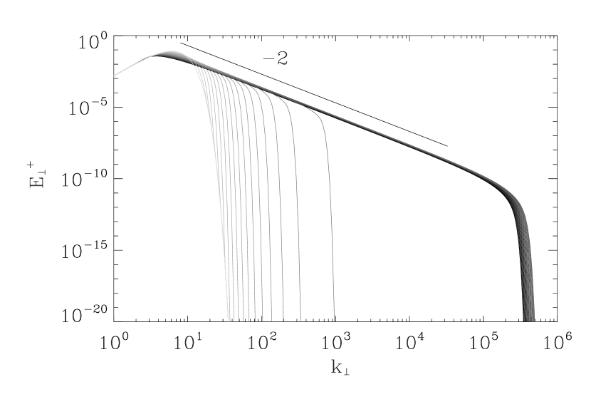
Figure 2: Time evolution of the energy spectrum $E^{+}_{\perp}(k_{\perp})$ for a cross-helicity $\rho=0$. The stationary spectrum is well fitted by a power law in $k_{\perp}^{-2}$. Forty spectra are shown with a constant interval of time.

The first simulation corresponds to the zero cross-helicity case for which by definition $E^{+}_{\perp}=E^{-}_{\perp}$. Large scale spectra centered around $k_{\perp}=k_{0}$ are taken initially with the form

$$E_{\perp}^{\pm}({k_{\perp}})\sim{k_{\perp}}^{3}\exp(-{k_{\perp}}^{2}/k_{0}^{2})\,,$$ (50)

where $k_{0}=5$. Only the time evolution of $E_{\perp}^{+}$ is given in Fig. 2. We see that the front of the energy spectrum propagates towards larger wavenumbers to reach eventually a $k_{\perp}^{-2}$–stationary spectrum as predicted by the theory. We may note the acceleration of the front until the dissipation scale is reached since spectra are separated by a constant interval of time. In the second simulation we have fixed initially the (reduced) cross-helicity to

$$\rho={E_{\perp}^{+}-E_{\perp}^{-}\over E_{\perp}^{+}+E_{\perp}^{-}}=0.8\,.$$ (51)

Like in the previous case the initial spectra are centered around $k_{\perp}=k_{0}=5$ with more energy in spectrum $E_{\perp}^{+}$ than in $E_{\perp}^{-}$. We keep the same form as (50). The result is shown in Fig. 3.

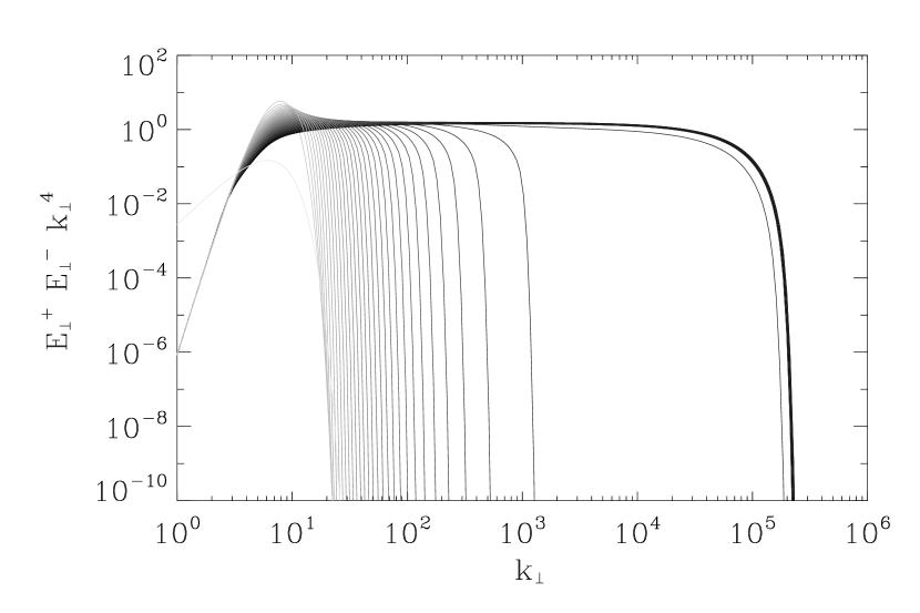
Figure 3: Time evolution of the compensated energy spectra $E^{+}_{\perp}E^{-}_{\perp}{k_{\perp}}^{4}$ for a cross-helicity $\rho=0.8$. The stationary spectra satisfy the relation $n_{+}+n_{-}=-4$. Forty spectra are shown with a constant interval of time.

We see that the compensated spectra fit well with the theoretical prediction $k_{\perp}^{-4}$ over several decades. In fact, spectra meet at relatively small $k_{\perp}$ and exhibit the same inertial range with the same ${k_{\perp}}^{-2}$–spectrum over a wide range of scales.

7 Discussion

It would be relevant to investigate if whether or nor the system recently derived by Matthaeus et al. (2009) for strong (anisotropic) MHD turbulence is able to recover the present equations when the limit of wave turbulence is taken. It would also be interesting to analyze if an anomalous scaling is detected during the front propagation (which is not easy to find here). We remind that the wave kinetic equations (14) exhibit a ${k_{\perp}}^{-7/3}$–spectrum during the non-stationary phase (at zero cross-helicity) which is still not understood (Galtier et al., 2000). Anomalous scalings are weaker in diffusion models of turbulence than in wave kinetic equations (Connaughton and Newell, 2010). We plan to further investigate this point by using for example a higher order numerical scheme. We also plan to further compare numerically the nonlinear diffusion equations and the wave kinetic equations to determine the domain of divergence between them or the influence of an external force (see e.g.  Galtier and Nazarenko, 2008).

The nonlinear diffusion equations for non-zero cross-helicity (30)–(32) is a simple and therefore useful system for describing a wide class of astrophysical plasmas. The solar corona with the myriad of magnetic loops which are characterized by a strong axial magnetic field is probably a good example of application of Alfvén wave turbulence (Rappazzo et al., 2007; Bigot et al., 2008b). This regime is also relevant for coronal holes where the solar wind is produced. For both examples, equations (30)–(32) could give a description of MHD turbulence at large scales since it seems inevitable that at smaller scales the strong turbulence regime overcomes. In this case a coupling with for example the advection-diffusion model proposed by Chandran (2008) would be relevant.

References

- Alexakis et al. (2007) Alexakis, A., Bigot, B., Politano, H., & Galtier, S. 2007, Phys. Rev. E, 76, 056313
- Bigot et al. (2008a) Bigot, B., Galtier, S., & Politano, H. 2008a, Phys. Rev. E, 78, 066301
- Bigot et al. (2008b) Bigot, B., Galtier, S., & Politano, H. 2008b, A&A, 490, 325
- Bigot et al. (2008c) Bigot, B., Galtier, S., & Politano, H. 2008c, Phys. Rev. Lett., 100, 074502
- Buchlin and Velli (2007) Buchlin, É., and Velli, M. 2007, ApJ, 662, 701
- Chae et al. (1998) Chae, J., Schühle, U., & Lemaire, P. 1998, ApJ, 505, 957
- Chandran (2005) Chandran, B.D.G. 2005, Phys. Rev. Lett., 95, 265004
- Chandran (2008) Chandran, B.D.G. 2008, ApJ, 685, 646
- Connaughton and Nazarenko (2004) Connaughton, C., & Nazarenko, S. 2004, Phys. Rev. Lett., 92, 044501
- Connaughton and Newell (2010) Connaughton, C., & Newell, A.C. 2010, Phys. Rev. E, 81, 036303
- Cranmer and van Ballegooijen (2003) Cranmer, S.R., & van Ballegooijen, A.A. 2003, ApJ, 594, 573
- Cranmer (2010) Cranmer, S.R. 2010, ApJ, 710, 676
- David et al. (1998) David, C., Gabriel, A.H., Bely-Dubau, F., Fludra, A., Lemaire, P., & Wilhelm, K. 1998, A&A, 336, L90
- Davidson (1958) Davidson, B. 1958, Neutron transport theory, Oxford University Press, Oxford, 1958
- Dyachenko et al. (1992) Dyachenko, S., Newell, A.C., Pushkarev, A.N., & Zakharov, V.E. 1992, Physica D, 57, 96
- Galtier (1999) Galtier, S. 1999, ApJ, 521, 483
- Galtier et al. (2000) Galtier, S., Nazarenko, S.V., Newell, A.C., & Pouquet, A. 2000, J. Plasma Phys., 63, 447
- Galtier et al. (2002) Galtier, S., Nazarenko, S.V., Newell, A.C., & Pouquet, A. 2002, ApJ, 564, L49
- Galtier (2006) Galtier, S. 2006, J. Plasma Phys., 72, 721
- Galtier and Chandran (2006) Galtier, S., & Chandran, B.D.G. 2006, Phys. Plasmas, 13, 114505
- Galtier (2008) Galtier, S. 2008, Phys. Rev. E, 77, 015302
- Galtier (2009) Galtier, S. 2009, Nonlin. Processes Geophys., 16, 83
- Galtier (2009) Galtier, S. 2009, ApJ, 704, 1371
- Galtier and Nazarenko (2008) Galtier, S., & Nazarenko, S.V. 2008, J. Turbulence, 9(40), 1
- Heisenberg (1948) Heisenberg, W. 1948, Proc. R. Soc. Lond. A, 195, 402
- Heyvaerts and Priest (1992) Heyvaerts, J., & Priest, E.R. 1992, ApJ, 390, 297
- Iroshnikov (1964) Iroshnikov, P. 1964, Sov. Astron., 7, 566
- Kolmogorov (1941) Kolmogorov, A.N. 1941, Dokl. Akad. Nauk SSSR, 32, 16
- Kraichnan (1963) Kraichnan, R.H. 1963, Phys. Fluids, 6, 1603
- Kraichnan (1965) Kraichnan, R.H. 1965, Phys. Fluids, 8, 1385
- Leith (1967) Leith, C.E. 1967, Phys. Fluids, 10, 1409
- Lithwick and Goldreich (2003) Lithwick, Y., & Goldreich, P. 2003, ApJ, 582, 1220
- MacBride et al. (2008) MacBride, B.T., Smith, C.W., & Forman, M.A. 2008, ApJ, 679, 1644
- Matthaeus et al. (1996) Matthaeus, W.H., Ghosh, S., Oughton, S., & Roberts, D.A. 1996, J. Geophys. Res., 101, 7619
- Matthaeus et al. (2009) Matthaeus, W.H., Oughton, S., & Zhou, Y. 2009, Phys. Rev. E, 79, 035401
- Mininni and Pouquet (2007) Mininni, P.D., & Pouquet, A. 2007, Phys. Rev. Lett., 99, 254502
- Orszag and Kruskal (1968) Orzsag, S.A., & Kruskal, M.D. 1968, Phys. Fluids, 11, 43
- Podesta (2009) Podesta, J.J. 2009, ApJ, 698, 986
- Pouquet et al. (1976) Pouquet, A., Frisch, U., & Léorat, J. 1976, J. Fluid. Mech., 77, 321
- Rappazzo et al. (2007) Rappazzo, A.F., Velli, M., Einaudi, G., & Dahlburg, R.B. 2007, ApJ, 657, L47
- Sahraoui et al. (2009) Sahraoui, F., Goldstein, M.L., Robert, P., & Khotyaintsev, Yu.V. 2009, Phys. Rev. Lett., 102, 231102
- Salem et al. (2009) Salem, C., Mangeney, A., Bale, S.D., & Veltri, P. 2009, ApJ, 702, 537
- Scalo and Elmegreen (2004) Scalo, J., & Elmegreen, B.G. 2004, ARA&A, 42, 275
- Smith et al. (2006) Smith, C.W., Hamilton, K., Vasquez, B.J., & Leamon, R.J. 2006, ApJ, 645, L85
- Zhou and Matthaeus (1990) Zhou, Y., & Matthaeus, W.H. 1990, J. Geophys. Res., 95, 14881