An Approximation Scheme for Reflected Stochastic Differential Equations

Abstract.

In this paper we consider the Stratonovich reflected stochastic differential equation $dX_{t}=\sigma(X_{t})\circ dW_{t}+b(X_{t})dt+dL_{t}$ in a bounded domain $\mathcal{O}$ which satisfies conditions, introduced by Lions and Sznitman, which are specified below. Letting $W^{N}_{t}$ be the $N$-dyadic piecewise linear interpolation of $W_{t}$ what we show is that one can solve the reflected ordinary differential equation $\dot{X}^{N}_{t}=\sigma(X^{N}_{t})\dot{W}^{N}_{t}+b(X^{N}_{t})+\dot{L}^{N}_{t}$ and that the distribution of the pair $(X^{N}_{t},L^{N}_{t})$ converges weakly to that of $(X_{t},L_{t})$. Hence, what we prove is a distributional version for reflected diffusions of the famous result of Wong and Zakai.

Perhaps the most valuable contribution made by our procedure derives from the representation of $\dot{X}^{N}_{t}$ in terms of a projection of $\dot{W}_{t}^{N}$. In particular, we apply our result in hand to derive some geometric properties of coupled reflected Brownian motion in certain domains, especially those properties which have been used in recent work on the “hot spots” conjecture for special domain.

1. Introduction

1.1. Motivation

As is well known, Itô stochastic differential equations can be very misleading from a geometric standpoint. The classic example of this observation is the Itô stochastic differential equation (SDE)

$$dX(t)=\sigma\bigl{(}X(t)\bigr{)}dW_{t}\text{ with }X(0)=\begin{pmatrix}1\\ 0\end{pmatrix}\text{ and }\sigma=\begin{pmatrix}-x_{2}\\ x_{1}\end{pmatrix},$$

where $W_{t}$ is a $1$-dimensional Brownian motion. If one makes the mistake of thinking that Itô differentials of Brownian motion behave like classical differentials, then one would predict the $X(t)$ should live on the unit circle. On the other hand, Itô’s formula, which is a quantitative statement of the extent to which they do not behave like classical differentials, says that $d|X(t)|^{2}=|X(t)|^{2}dt$, and so $|X(t)|^{2}=e^{t}$.

To avoid the sort of misinterpretation to which Itô SDE’s lead, it is convenient to replace Itô SDE’s by their Stratonvich counterparts. When one does so, then the Wong–Zakai theorem  [14] shows that the solution to the SDE can be approximated by solutions to the ordinary differential equation (ODE) which one obtains by piecewise linearizing the Brownian paths. In this way, one can transfer to solutions of the SDE geometric properties which one knows for the solutions to the ODE’s. The purpose of this paper is to carry out the analogous program for SDE’s for diffusions which are reflected at the boundary of some region. This is not the first time that such a program has been attempted. For example, R. Petterson proved in  [7] a result of this sort under the assumption that the domain is convex. Unfortunately, convexity is too rigid a requirement for applications of the sort which appear in papers like  [2] by Banuelos and Burdzy, and so it is important to replace convexity by a more general condition, like the one given in  [6] by A. Sznitman and P.L. Lions. Finally, it should be mentioned that the article  [5] by A. Kohatsu-Higa contains a very general, highly abstract approximation procedure which may be applicable to the situation here.

1.2. Background for Reflected SDE’s

We begin by recalling the (deterministic) Skorohod problem.

Let $\mathcal{O}\subset\mathbb{R}^{d}$ be a domain and to each $x\in\partial\mathcal{O}$ assign a nonempty collection $\nu(x)\subseteq\mathbb{S}^{d-1}$, to be thought of as the set of directions in which a path can be “pushed” when it hits $x$. Given a continuous path $w:[0,\infty)\rightarrow\mathbb{R}^{d}$ with $w_{0}\in\mathcal{O}$, known as the “input,” we say that a solution to the Skorohod problem for $(\mathcal{O},\nu(x))$ is a pair $(x_{\cdot},\ell_{\cdot})$ consisting of a continuous path $t\in[0,\infty)\longmapsto x_{t}\in\bar{\mathcal{O}}$ and a continuous function of locally bounded variation $t\in[0,\infty)\longmapsto\ell_{t}\in\mathbb{R}^{d}$ such that

(1) $$x_{t}=w_{t}+\ell_{t},\;|\ell|_{t}=\int_{0}^{t}1_{\partial\mathcal{O}}(x_{s})d|\ell|_{s},\text{ and }\ell_{t}=\int_{0}^{t}\nu(x_{s})d|\ell|_{s},$$

where $|\ell|_{t}$ denotes the total variation of $\ell_{t}$ on the interval $[0,t]$, and the third line is a shorthand way of saying that

$$\frac{d\ell_{t}}{d|\ell|_{t}}\in\nu(x_{t}),\quad d|\ell|_{t}-\text{a.e.}.$$

When a unique solution exists for each input, we will call the map $w_{\cdot}\rightsquigarrow(x_{\cdot},\ell_{\cdot})$ the Skorohod map and will denote it by $\Gamma$. Also, the path $x_{\cdot}$ will be referred to as the “output.”

Throughout this paper we will take $\nu(x)$ to be the collection of inward pointing proximal normal vectors

(2) $$\nu(x)\equiv\big{\{}\nu\in\mathbb{S}^{d-1}:\exists C>0\;\forall x^{\prime}\in\bar{\mathcal{O}}\;(x^{\prime}-x)\cdot\nu+C|x-x^{\prime}|^{2}\geq 0\}.$$

Elementary algebra shows that

(3) $$(x^{\prime}-x)\cdot\nu+C|x-x^{\prime}|^{2}<0\Longleftrightarrow\left|x^{\prime}-(x-\frac{\nu}{2C})\right|^{2}<\left(\frac{1}{2C}\right)^{2}$$

which shows that, geometrically, $\nu(x)$ is the collection of unit vectors based at $x\in\partial\mathcal{O}$ such that there exists an open ball touching the base of $\nu$ but not intersecting $\mathcal{O}$.

The class of domains which we will consider was described by Lions and Sznitman in [6]. Namely, we will say that $\mathcal{O}$ is admissible if

Definition 1.1.

1. $\forall x\in\partial\mathcal{O}$, $\nu(x)\neq\phi$, and there exists a $C_{0}\geq 0$ such that

   $$(x^{\prime}-x)\cdot\nu+C_{0}|x-x^{\prime}|^{2}\geq 0\text{ for all }x^{\prime}\in\mathcal{O},\;x\in\partial\mathcal{O},\text{ and }\nu\in\nu(x).$$

2. There exists a function $\phi\in C^{2}(\mathbb{R}^{d};\mathbb{R})$ and $\alpha>0$ such that

   $$\nabla\phi(x)\cdot\nu\geq\alpha>0\text{ for all }x\in\partial\mathcal{O}\text{ and }\nu\in\nu(x).$$

3. There exist $n\geq 1$, $\lambda>0$, $R>0$, $a_{1},\ldots,a_{n}\in\mathbb{S}^{d-1}$, and $x_{1},\ldots,x_{n}\in\partial O$ such that

   $$\begin{gathered}\partial O\subseteq\bigcup_{i=1}^{n}B(x_{i},R)\text{ and }\\ x\in\partial O\cap B(x_{i},2R)\Longrightarrow\nu\cdot a_{i}\geq\lambda>0\text{ for all }\nu\in\nu(x).\end{gathered}$$

In view of (3), Part 1 of Definition 1.1 can be seen as a sort of uniform exterior ball condition. More precisely, it says that not only can every point $x\in\partial\mathcal{O}$ can be touched by an exterior ball but also that the exterior ball touching $x$ can be scaled to have a uniformly large radius. In the convex analysis literature, the closure of a set $\mathcal{O}$ satisfying Part 1 of Definition 1.1 is said to be uniformly prox-regular (See [8], especially Theorem 4.1, for more on the properties of uniformly prox-regular sets).

Parts 2 and 3 of Definition 1.1 are regularity requirements on $\partial\mathcal{O}$ which ensure that the “normal vectors” don’t fluctuate too wildly. In this connection, notice that Part 3 is implied by Part 2 when $\mathcal{O}$ is bounded.

In their paper [6], Lions and Sznitman show that for each $w_{\cdot}\in C\bigl{(}[0,\infty);\mathbb{R}^{d}\bigr{)}$ there exists an almost surely unique solution $(x_{\cdot},\ell_{\cdot})$ to the deterministic Skorohod problem when the domain $\mathcal{O}$ is admissible. The map $\Gamma$ which takes $w_{\cdot}$ to $x_{\cdot}$ is called the deterministic Skorohod map.

We turn next to the formulation of reflected diffusions in terms of a Skorohod problem for an SDE. Until further notice, we will be looking at Itô SDE’s and will only reformulate them as Stratonovich SDE’s when it is important to do so.

Let $\mathcal{O}\subset\mathbb{R}^{d}$ an admissible domain, and let $\sigma:\bar{\mathcal{O}}\longrightarrow\rm{Hom}(\mathbb{R}^{r};\mathbb{R}^{d})$ and $b:\bar{\mathcal{O}}\longrightarrow\mathbb{R}^{d}$ be uniformly Lipschitz continuous maps. Given an $r$-dimensional Brownian motion $W_{\cdot}$ and $x_{0}\in\mathcal{O}$, a solution to $(X_{\cdot},L_{\cdot})$ to the reflected SDE (4) is a continuous process $\bigl{\{}(X_{t},L_{t}):\,t\geq 0\bigr{\}}$ which is progressively measurable with respect to $W_{\cdot}$ and satisfies the conditions that $(X_{t},L_{t})\in\bar{\mathcal{O}}\times\mathbb{R}^{d}$ and $|L|_{t}<\infty$ for all $t\geq 0$, and, almost surely,

(4) $$\begin{split}X_{t}=&x_{0}+\int_{0}^{t}\sigma(X_{s})dW_{s}+\int_{0}^{t}b(X_{s})ds+L_{t},\\ |L|_{t}=&\int_{0}^{t}1_{\partial\mathcal{O}}(X_{s})d|L|_{s},\text{ and }L_{t}=\int_{0}^{t}\nu(X_{s})d|L|_{s},\end{split}$$

where $|L|_{t}$ denotes the total variation of $L_{t}$ by time $t$, and the third line is shorthand for $\frac{dL_{t}}{d|L|_{t}}\in\nu(x_{t}),\;d|L|_{t}-\text{a.e.}$.

Existence and uniqueness of solution to reflected SDE’s was proved by H. Tanaka in  [12] when $\mathcal{O}$ is convex. The extension of his result to admissible domains was made by Lions and Sznitman in  [6] and Saisho in  [10]. We refer the reader to those papers for an overview of the subject.

2. Equations with Reflection

2.1. Properties of Solutions to Reflected ODE’s

Suppose that $\mathcal{O}$ is a bounded, admissible domain and that $\sigma:\bar{\mathcal{O}}\longrightarrow\rm{Hom}(\mathbb{R}^{r};\mathbb{R}^{d})$ is uniformly Lipschitz continuous. In this section we will show that, for each $x_{0}\in\bar{\mathcal{O}}$ and $w_{\cdot}\in C\bigl{(}[0,\infty);\mathbb{R}^{d}\bigr{)}$ there is precisely one solution $(x_{\cdot},\ell_{\cdot})$ to the reflected ODE

(5) $$\begin{split}x_{t}=&x_{0}+\int_{0}^{t}\sigma(x_{s})dw_{s}+\ell_{t},\\ |\ell|_{t}=&\int_{0}^{t}1_{\partial\mathcal{O}}(x_{s})d|\ell|_{s},\text{ and }\ell_{t}=\int_{0}^{t}\nu(x_{s})d|\ell|_{s},\end{split}$$

where $x_{\cdot}\in C\bigl{(}[0,\infty);\bar{\mathcal{O}}\bigr{)}$ and $\ell_{t}:[0,\infty)\longrightarrow\mathbb{R}^{d}$ is a continuous function having finite variation $|\ell|_{t}$ on $[0,t]$ for all $t>0$. In addition, we will give a geometrically appealing alternate description of this solution. Previously, existence and uniqueness results for variants of (5) are well known in the convex analysis literature. For example, see [3] for a recent such result as well as a good overview of other known results.

Although the proofs of existence and uniqueness are implicit in the contents of other articles, we, mimicking the proof of Theorem 3.1 in [6], will prove them here. For this purpose, consider the map $F_{w}:C\bigl{(}[0,\infty);\bar{O}\bigr{)}\longrightarrow C\bigl{(}[0,\infty);\bar{O}\bigr{)}$ given by $F_{w}(y_{\cdot})=\Gamma(x_{0}+\int_{0}^{\cdot}{\sigma(y_{s})dw_{s}})$, where $\Gamma$ is the Skorohod map. We will show that $F$ has a unique fixed point, and the key to doing so is contained in the next lemma.

Lemma 2.1.

For each $T>0$ there exists a $C=C_{w}(T)<\infty$ such that for any pair of paths $y_{\cdot}$ and $y^{\prime}_{\cdot}$,

(6) $$|F_{w}(y_{\cdot})_{t}-F(y^{\prime}_{\cdot})_{t}|^{2}\leq\int_{0}^{t}e^{C(t-\tau)}|y_{\tau}-y^{\prime}_{\tau}|^{2}d\tau\quad\text{for all }t\in[0,T].$$

Proof.

Set $z_{\cdot}=F(y_{\cdot})$ and $z^{\prime}_{\cdot}=F(y^{\prime}_{\cdot})$. Given $T>0$, we will show that there is a $C<\infty$ such that

$$|z_{t}-z^{\prime}_{t}|^{2}\leq C\left(\int_{0}^{t}|z_{\tau}-z^{\prime}_{\tau}|^{2}\,d\tau+\int_{0}^{t}|y_{\tau}-y^{\prime}_{\tau}|^{2}\,d\tau\right),\quad t\in[0,T].$$

Once this is proved, the required estimate follows immediately from Gromwall’s inequality.

Let $\phi$ be the function associated with $\mathcal{O}$ (see part 2 of Definition 1.1). For any constant $\gamma$, we have that

$$e {}^{-\gamma[\phi(z_{t})+\phi(z^{\prime}_{t})]}d\bigl{(}e^{\gamma[\phi(z_{t})+\phi(z^{\prime}_{t})]}|z_{t}-z^{\prime}_{t}|^{2}\bigr{)}$$

$$= 2(z_{t}-z^{\prime}_{t})\cdot\bigl{[}\bigl{(}\sigma(y_{t})dw_{t}+d\ell_{t}\bigr{)}-\bigl{(}\sigma(y^{\prime}_{t})dw_{t}+d\ell^{\prime}_{t}\bigr{)}\bigr{]}$$

$$+|z_{t}-z^{\prime}_{t}|^{2}\gamma\bigl{[}\nabla\phi(z_{t})\cdot\bigl{(}\sigma(y_{t})dw_{t}+d\ell_{t}\bigr{)}+\nabla\phi(z^{\prime}_{t})\cdot\bigl{(}\sigma(y^{\prime}_{t})dw_{t}+d\ell^{\prime}_{t}\bigr{)}\bigr{]}$$

$$= \bigl{[}(2(z_{t}-z^{\prime}_{t})+\gamma|z_{t}-z^{\prime}_{t}|^{2}\nabla\phi(z_{t}))\cdot\nu(z_{t})\bigr{]}d|\ell|_{t}$$

$$+\bigl{[}(2(z^{\prime}_{t}-z_{t})+\gamma|z_{t}-z^{\prime}_{t}|^{2}\nabla\phi(z^{\prime}_{t}))\cdot\nu(z^{\prime}_{t})\bigr{]}d|\ell^{\prime}|_{t}$$

$$+\bigl{[}2(z_{t}-z^{\prime}_{t})\cdot\bigl{(}\sigma(y_{t})-\sigma(y^{\prime}_{t})\bigr{)}+\gamma|z_{t}-z^{\prime}_{t}|^{2}\bigl{(}\nabla\phi(z_{t})\sigma(y_{t})+\nabla\phi(z^{\prime}_{t})\sigma(y^{\prime}_{t})\bigr{)}\bigr{]}dw_{t}$$

Taking $\gamma=\frac{-2C_{0}}{\alpha}$, we have that (cf. Part 1 of Definition 1.1) the first two terms are less than or equal to $0$. Since $\sigma$ and $\nabla\phi$ are Lipschitz continuous and $\frac{dw}{dt}$ is bounded on finite intervals, we know that there exists a $C=C_{w}(T)<\infty$ such that

$$|z_{t}-z^{\prime}_{t}|^{2}\leq C\left(\int_{0}^{t}|z_{\tau}-z^{\prime}_{\tau}|^{2}d\tau+\int_{0}^{t}|z_{\tau}-z^{\prime}_{\tau}||y_{\tau}-x^{\prime}_{\tau}|d\tau+\int_{0}^{t}|y_{\tau}-y^{\prime}_{\tau}|^{2}d\tau\right)$$

for $t\in[0,R]$. Thus, because $|z_{\tau}-z^{\prime}_{\tau}||y_{\tau}-y^{\prime}_{\tau}|\leq\frac{1}{2}|z_{\tau}-z^{\prime}_{\tau}|^{2}+\frac{1}{2}|y_{\tau}-y^{\prime}_{\tau}|^{2}$, we get our estimate after replacing $C$ by $2C$. ∎

Once we have Lemma 2.1, one can apply a standard Picard iteration argument to show that $F_{w}$ has a unique fixed point and that this fixed point is the first component of the one and only pair $(x_{t},\ell_{t})$ which solves (5).

We now want to describe a couple of important properties of the solution $(x_{\cdot},\ell_{\cdot})$.

Lemma 2.2.

Let $(x_{\cdot},\ell_{\cdot})$ be the solution to (5) for a given input $w_{\cdot}$ and starting point $x_{0}\in\bar{\mathcal{O}}$. Then there exists a constant $C$, depending only on $\sigma$, $b$, and $\mathcal{O}$, such that

$$d|x|_{t}\leq Cd|w|_{t}$$

Proof.

Set $y_{t}=x_{0}+\int_{0}^{t}\sigma(x_{s})dw_{s}$. Then, $x_{\cdot}=\Gamma(y_{\cdot})$, and so it follows from Theorem 2.2 in [6] that $d|\ell|_{t}\leq d|y|_{t}$. Since $\sigma$ is bounded on $\bar{\mathcal{O}}$, there exists a $C<\infty$ such that $d|y|_{t}\leq Cd|w|_{t}$, and therefore, because $x_{t}=y_{t}+\ell_{t}$, we have that $d|x|_{t}\leq d|y|_{t}+d|\ell|_{t}\leq C\bigl{(}d|w|_{t}+d|w|_{t}\bigr{)}$, from which the lemma follows immediately. ∎

We now introduce a more geometric representation of the equation (5). For a closed set $D\subseteq\mathbb{R}^{d}$ and $z\in\mathbb{R}^{d}$, let $d_{D}(z)\equiv\inf_{y\in D}|y-z|$ denote the distance from $z$ to $D$ and denote by

$$T_{D}(z)\equiv\{v\in\mathbb{R}^{d}:\liminf_{h\searrow 0}\frac{d_{D}(z+hv)}{h}=0\}$$

the tangent cone (a.k.a. the contingent cone) to $D$ at $z$. Finally, let $\text{{\rm proj}}_{D}(z)$ denote the (possibly multi-valued) projection of $z$ onto $D$.

The following is a version of a representation result which was introduced originally in [4].

Theorem 2.3.

Let $\mathcal{O}$ be a bounded, admissible set and $w_{\cdot}$ a fixed, piecewise smooth input. If $(x_{\cdot},\ell_{\cdot})$ is the unique solution to (5), then

(7) $$\dot{x}_{t}=\text{{\rm proj}}_{T_{\bar{\mathcal{O}}}(x_{t})}(\sigma(x_{t})\dot{w}_{t}),\quad t\text{-a.e.}$$

Conversely, given a solution $x_{\cdot}$ to (7), there exists an $\ell_{\cdot}$ such that $(x_{\cdot},\ell_{\cdot})$ is a solution to (5).

Remark 2.4.

In general, the tangent cone $T_{D}(z)$ is only closed and not necessarily convex. However, Part 1 of Definition 1.1 guarantees that $T_{\bar{\mathcal{O}}}(z)$ is convex for all $z\in\bar{\mathcal{O}}$ (cf. Lemma 2.5 below) and so $\text{{\rm proj}}_{K}(\cdot)$ is single valued.

In order to prove Theorem 2.3, we will need to introduce some concepts from convex analysis. For more information about these concepts and their properties, we refer the reader to the texts [9] and [13].

A non-empty set $K\subseteq\mathbb{R}^{d}$ is called a cone if $v\in K\Longrightarrow\lambda v\in K$ for all $\lambda\geq 0$. Given a cone $K$, we denote by $K^{*}$ its polar cone $K^{*}$ to be the set $\{w:v\cdot w\leq 0,\;\forall v\in K\}$. Next, for a given closed set $D\subseteq\mathbb{R}^{d}$ and a $z\in D$, we define the proximal normal cone to $D$ at $z$ to be the set

$$N^{p}_{D}(z)\equiv\{v\in\mathbb{R}^{d}:\exists C>0\text{ s.t. }(y-z)\cdot\nu\leq C|z-y|^{2},\quad\forall y\in D\}$$

and the Clarke tangent cone to $D$ at $z$ to be the set

$$\hat{T}_{D}(z)\equiv\{v\in\mathbb{R}^{d}:\forall z_{n}\in D\text{ s.t. }z_{n}\rightarrow z,\quad\exists v_{n}\in T_{D}(z_{n})\text{ s.t. }v_{n}\rightarrow v\}.$$

Note that $\hat{T}_{D}(z)$ is always convex.

We now present a lemma which records the properties of an admissible set $\mathcal{O}$ in terms of these concepts.

Lemma 2.5.

Let $\mathcal{O}$ be admissible. Then

1. For each $z\in\partial\mathcal{O}$,

   $$v\in N^{p}_{\bar{\mathcal{O}}}(z)\Longleftrightarrow\frac{-v}{|v|}\in\nu(z)\text{ for }v\neq 0$$

2. The graph of $z\longrightarrow N^{p}_{\bar{\mathcal{O}}}(z)$ is closed. That is, if $z_{i}\in\bar{\mathcal{O}}$, $v_{i}\in N^{p}_{\bar{\mathcal{O}}}(z_{i}),z_{i}\rightarrow z,$ and $v_{i}\rightarrow v$, then $v\in N^{p}_{\bar{\mathcal{O}}}(z)$.

3. $T_{\bar{\mathcal{O}}}(z)=\hat{T}_{\bar{\mathcal{O}}}(z)$, and so it is convex for all $z\in\bar{\mathcal{O}}$.

4. $N^{p}_{\bar{\mathcal{O}}}(z)=T_{\bar{\mathcal{O}}}(z)^{*}$ for all $z\in\bar{\mathcal{O}}$.

Proof.

1. is immediate from our definitions.

2. follows from 1. and Part 1 of Definition 1.1. Indeed, there exists a $C_{0}>0$ such that for each $i$,

(8) $$(z_{i}-y)\cdot v_{i}+C_{0}|v_{i}||z_{i}-y|^{2}\geq 0,\quad\forall y\in\bar{\mathcal{O}}$$

(note that when $z_{i}\in\mathcal{O}$, $v_{i}=0$ and (8) holds trivially). Taking $i\rightarrow\infty$ we see that $(z-y)\cdot v+C_{0}|v||z-y|^{2}\geq 0$ for all $y\in\bar{\mathcal{O}},$ from which it follows that $v\in N^{p}_{\bar{\mathcal{O}}}(z)$.

3. and 4. follow in a standard way from 2. See Chapter 4. of [13] and Chapter 6 of [9] (in particular Corollary 6.29) for the details. ∎

Using ideas from [4], we now prove Theorem 2.3.

Proof.

(Proof of Theorem 2.3) First suppose $(x_{\cdot},\ell_{\cdot})$ is a solution to (5). From Theorem 2.2 and its proof, we see that $x_{\cdot}$ and $\ell_{\cdot}$ are locally Lipschitz and therefore that $\dot{x}_{t}=\sigma(x_{t})\dot{w}_{t}+\dot{\ell}_{t},\;t\text{-a.e.}$ Since $x_{t+h}$ and $x_{t-h}$ are in $\bar{\mathcal{O}}$, we have that

(9) $$\dot{x}_{t}\in-T_{\bar{\mathcal{O}}}(x_{t})\cap T_{\bar{\mathcal{O}}}(x_{t}),\quad t\text{-a.e.},$$

and, because $T_{\bar{\mathcal{O}}}(x_{t})$ is convex, $\dot{x}_{t}$ is the projection of $\sigma(x_{t})\dot{w}_{t}$ onto $T_{\bar{\mathcal{O}}}(x_{t})$ if and only if $\bigl{(}\sigma(x_{t})\dot{w}_{t}-\dot{x}_{t})\cdot(v-\dot{x}_{t}\bigr{)}\leq 0$ for all, $v\in T_{\bar{\mathcal{O}}}(x_{t})$. Note that by property 1. of Lemma 2.5, $-\dot{\ell}_{t}\in N^{p}_{\bar{\mathcal{O}}}(x_{t})$ (when $x_{t}\in\mathcal{O}$ this holds trivially), and so, by property 4. of Lemma 2.5 and (9), we have that

$$\dot{x}_{t}\cdot\dot{\ell}_{t}\leq 0,\quad\dot{x}_{t}\cdot\dot{\ell}_{t}\geq 0\Longrightarrow\dot{x}_{t}\cdot\dot{\ell}_{t}=0.$$

Therefore, using property 4. again, we have that

$$(\sigma(x_{t})\dot{w}_{t}-\dot{x}_{t})\cdot(v-\dot{x}_{t})=-\dot{\ell}_{t}\cdot(v-\dot{x}_{t})=-\dot{\ell}_{t}\cdot v\leq 0$$

as desired.

Conversely, suppose $x_{\cdot}$ is a solution to (7), and set $\ell_{t}\equiv\int_{0}^{t}\dot{x}_{s}-\sigma(x_{s})\dot{w}_{s}ds$. Then $\ell_{0}=0$ and, since $\sigma$ is bounded, $\ell_{\cdot}$ is a continuous function of locally bounded variation. Finally, because $\dot{x}_{t}$ is the projection of $\sigma(x_{t})\dot{w}_{t}$ onto the convex set $T_{\bar{\mathcal{O}}}(x_{t})$, we have that

$$-\dot{\ell}_{t}\cdot(v-\dot{x}_{t})=(\sigma(x_{t})\dot{w}_{t}-\dot{x}_{t})\cdot(v-\dot{x}_{t})\leq 0,\quad\forall v\in T_{\bar{\mathcal{O}}}(x_{t}).$$

Since $\dot{x}_{t}\in T_{\bar{\mathcal{O}}}(x_{t})$ and $T_{\bar{\mathcal{O}}}(x_{t})$ is a convex cone, for each $v\in T_{\bar{\mathcal{O}}}(x_{t})$, $x_{t}+v\in T_{\bar{\mathcal{O}}}(x_{t})$. Thus, by replacing $v$ with $v+x_{t}$ in the inequality above, we find that $-\dot{\ell}_{t}\cdot v\leq 0$ for all $v\in T_{\bar{\mathcal{O}}}(x_{t})$, and so $-\dot{\ell}_{t}\in T_{\bar{\mathcal{O}}}(x_{t})^{*}=N^{p}_{\bar{\mathcal{O}}}(x_{t})$. Finally, by property 1. of Lemma 2.5, this implies that $(x_{t},\ell_{t})$ is a solution to (5). ∎

3. Tightness of the Approximating Measures

Let $\bigl{(}C([0,\infty);\mathbb{R}^{r}),\mathcal{F},\mathbb{W}\bigr{)}$ be the standard $r$-dimensional Wiener space. That is, $\mathcal{F}$ is the Borel field for $C([0,\infty);\mathbb{R}^{r})$ and $\mathbb{W}$ is the standard Wiener measure. We will use $W_{\cdot}$ to denote a generic Wiener path and $\mathcal{F}_{t}$ to denote the $\sigma$-algebra generated by $W_{\cdot}\restriction[0,t]$. Finally, for each positive integer $N$, let $W^{N}_{\cdot}$ denote the $N$-dyadic linear polygonalization of $W_{\cdot}$. That is, $W^{N}_{m2^{-N}}=W_{m2^{-N}}$ and $W^{N}_{\cdot}$ is linear on $[m2^{-N},(m+1)2^{-N}]$ for each $m\in\mathbb{N}$.

Next, $\mathcal{O}\subset\mathbb{R}^{d}$ will be a bounded, admissible domain, and $b:\bar{\mathcal{O}}\longrightarrow\mathbb{R}^{d}$ and $\sigma:\bar{\mathcal{O}}\longrightarrow\rm{Hom}(\mathbb{R}^{r};\mathbb{R}^{d})\bigr{)}$ will be uniformly Lipschitz continuous functions. Given a starting point $x_{0}\in\bar{\mathcal{O}}$, for each $W^{N}_{\cdot}$, $(X^{N}_{\cdot},L^{N}_{\cdot})$ will denote the solution to the reflected ODE (5) with $w_{t}$ and $\sigma(x)$ replaced by, respectively,

$$\begin{pmatrix}W^{N}_{t}\\ t\end{pmatrix}\in\mathbb{R}^{r}\times\mathbb{R}\quad\text{and}\quad\begin{pmatrix}\sigma(x)\\ b(x)\end{pmatrix}\in\rm{Hom}\bigl{(}\mathbb{R}^{r}\times\mathbb{R};\mathbb{R}^{d}\times\mathbb{R}).$$

$\{X^{N}_{t}:\,t\geq 0\}$ and $\{L^{N}_{t}:\,t\geq 0\}$ are then progressively measurable with respect to $\{\mathcal{F}_{t}:\,t\geq 0\}$, and we will use $\mathbb{P}^{N}$ on the $(X,L,W)$-pathspace $C\bigl{(}[0,\infty);\bar{\mathcal{O}}\bigr{)}\times C\bigl{(}[0,\infty);\mathbb{R}^{d}\bigr{)}\times C\bigl{(}[0,\infty);\mathbb{R}^{r}\bigr{)}$ to denote the distribution of the triple $(X^{N}_{t},L^{N}_{t},W^{N}_{t})$ under $\mathbb{W}$.

In first subsection, we show that the family $\{\mathbb{P}^{N}:\,N\geq 0\}$ is tight on the $(X,L,W)$-pathspace. In second subsection, we also develop some estimates which will needed for the next section.

3.1. Tightness of the ${\mathbb{P}}^{N}$

By Kolmogorov’s Continuity Criterion, we will know that $\{\mathbb{P}^{N}:\,N\geq 0\}$ is tight as soon as we prove that for each $m\in{\mathbb{N}}$ and $T>0$ there exists a $C_{m}(T)<\infty$, which is independent of $N$, such that

(10) $$\mathbb{E}\bigl{[}|W^{N}_{t}-W^{N}_{s}|^{2^{m+1}}\bigr{]} \leq C_{m}(T)(t-s)^{2^{m}}$$

(11) $$\mathbb{E}\bigl{[}|X^{N}_{t}-X^{N}_{s}|^{2^{m+1}}\bigr{]} \leq C_{m}(T)(t-s)^{2^{m}}$$

(12) $$\mathbb{E}\bigl{[}|L^{N}_{t}-L^{N}_{s}|^{2^{m+1}}\bigr{]} \leq C_{m}(T)(t-s)^{2^{m}}.$$

First note that (10) is an easy consequence of the equality $\mathbb{E}\bigl{[}|W_{t}-W_{s}|^{2^{m+1}}\bigr{]}=C_{m}(t-s)^{2^{m}}$ where $C_{m}=\mathbb{E}\bigl{[}|W_{1}|^{2^{m+1}}\bigr{]}$.

The proofs of (11) and (12) are a little more involved.

Lemma 3.1.

There is a $C<\infty$ such that for all $s<t\leq s+2^{-N}$,

(13) $$|X^{N}_{t}-X^{N}_{s}|\leq C|W^{N}_{t}-W^{N}_{s}|+C(t-s)$$

Proof.

When $s$ and $t$ lie in the same $N$-dyadic interval, this follows more or less immediately from Theorem 2.2. Namely,

$$|X^{N}_{t}-X^{N}_{s}| \leq|X^{N}|_{t}-|X^{N}|_{s}\leq C\bigl{(}(|W^{N}|_{t}-|W^{N}|_{s})+(t-s)\bigr{)}$$

$$=C\bigl{(}|W^{N}_{t}-W^{N}_{s}|+(t-s)\bigr{)},$$

where the last equality comes from the fact that $s$ and $t$ lie in the same $N$-dyadic interval. When they are in adjacent $N$-dyadic intervals, one can reduce to the case when they are in the same $N$-dyadic interval by an application of Minkowski’s inequality. ∎

It remains to handle $s$ and $t$ with $t-s>2^{-N}$, and for this we will need the next two lemmas. Here, and elsewhere, ${\lfloor u\rfloor}$ is shorthand for the largest $N$-dyadic number $m2^{-N}$ dominated by $u$. That is, ${\lfloor u\rfloor}$ equals $2^{-N}$ times the integer part of $2^{N}u$.

Lemma 3.2.

For $m\geq 0$ there exists a $C_{m}<\infty$ such that for all $s<t$

(14) $$\mathbb{E}\left[\left(\int_{s}^{t}|W^{N}_{u}-W^{N}_{\lfloor u\rfloor}|\ d|W^{N}|_{u}\right)^{2^{m}}\right]\leq C_{m}(t-s)^{2^{m}}$$

and

(15) $$\mathbb{E}\left[\left(\int_{s}^{t}(u-{\lfloor u\rfloor})\ d|W^{N}|_{u}\right)^{2^{m}}\right]\leq C_{m}(t-s)^{2^{m}}$$

Proof.

If $s<t$ lie in the same $N$-dyadic interval we have that

$$\int_{s}^{t}|W^{N}_{u}-W^{N}_{\lfloor u\rfloor}|d|W^{N}|_{u}= 4^{N}|\Delta W^{N}_{\lfloor s\rfloor}|^{2}\int_{s}^{t}(u-{\lfloor u\rfloor})du\leq 2^{N}|\Delta W^{N}_{\lfloor s\rfloor}|^{2}(t-s)$$

$$\int_{s}^{t}(u-{\lfloor u\rfloor})d|W^{N}|_{u}= 2^{N}|\Delta W^{N}_{\lfloor s\rfloor}|\int_{s}^{t}(u-{\lfloor u\rfloor})du\leq|\Delta W^{N}_{\lfloor s\rfloor}|(t-s)$$

and so

(16) $$\mathbb{E}\left[\left(\int_{s}^{t}|W^{N}_{u}-W^{N}_{\lfloor u\rfloor}|d|W^{N}|_{u}\right)^{2^{m}}\right]^{2^{-m}}\leq C_{m}(t-s)$$

$$\mathbb{E}\left[\left(\int_{s}^{t}(u-{\lfloor u\rfloor})d|W^{N}|_{u}\right)^{2^{m}}\right]^{2^{-m}}\leq C_{m}2^{-N2^{m-1}}(t-s)\leq C_{m}(t-s).$$

Applying the Minkowski inequality, we see that the inequalities (16) continue to hold for general $s<t$. ∎

Lemma 3.3.

Let $\phi$ and $\alpha$ be as in Part 2 of Definition 1.1, and set $\gamma=-\frac{2C_{0}}{\alpha}$, where $C_{0}$ is the constant in Part 1 of that definition. Given $s\geq 0$, there exist $\{\mathcal{F}_{t}:\,t\geq 0\}$ progressively measurable functions $\{Z_{\tau,s}:\,\tau\geq s\}$ and $\{V_{\tau,s}:\,\tau\geq s\}$ satisfying

(17) $$|Z^{N}_{u,s}|\leq C|X^{N}_{u}-X^{N}_{s}|,\text{ }|Z^{N}_{u_{2},s}-Z^{N}_{u_{1},s}|\leq C|X^{N}_{u_{2}}-X^{N}_{u_{1}}|,\text{ and }|V^{N}_{u,s}|\leq C,$$

with a constant $C<\infty$, which is independent of $s$ and $N$, such that

(18) $$e^{\gamma\phi(X^{N}_{t})}|X^{N}_{t}-X^{N}_{s}|^{2}\leq\int_{s}^{t}Z^{N}_{u,s}dW^{N}_{u}+\int_{s}^{t}V^{N}_{u,s}du\text{ for all }t>s.$$

Proof.

Just as in the proof of Lemma 2.1,

$$d\bigl{(}e^{\gamma\phi(X^{N}_{t})} |X^{N}_{t}-X^{N}_{s}|^{2}\bigr{)}$$

$$\leq e^{\gamma\phi(X^{N}_{t})}\Bigl{(}2(X^{N}_{t}-X^{N}_{s})+\gamma|X^{N}_{t}-X^{N}_{s}|^{2}\nabla\phi(X^{N}_{t})\Bigr{)}\sigma(X^{N}_{t})dW^{N}_{t}$$

$$+e^{\gamma\phi(X^{N}_{t})}\Bigl{(}2(X^{N}_{t}-X^{N}_{s})+\gamma|X^{N}_{t}-X^{N}_{s}|^{2}\nabla\phi(X^{N}_{t})\Bigr{)}b(X^{N}_{t})dt.$$

from which (18) follows with

$$Z^{N}_{u,s}=e^{\gamma\phi(X^{N}_{u})}\Bigl{(}2(X^{N}_{u}-X^{N}_{s})+|X^{N}_{u}-X^{N}_{s}|^{2}\gamma\nabla\phi(X^{N}_{u})\Bigr{)}\sigma(X^{N}_{u})$$

and

$$V^{N}_{u,s}=e^{\gamma\phi(X^{N}_{u})}\Bigl{(}2(X^{N}_{u}-X^{N}_{s})+|X^{N}_{u}-X^{N}_{s}|^{2}\gamma\nabla\phi(X^{N}_{u})\Bigr{)}\cdot b(X^{N}_{u}).$$

Since $\nabla\phi$, $b$, and $\sigma$ are Lipschitz continuous functions on the bounded domain $\mathcal{O}$, it is clear how to choose the $C$ in (17). ∎

We now prove (11) in the case that $t-s>2^{-N}$ by induction on $m$. Taking into account the fact that $\phi$ is bounded, we can use (18) to derive the estimate

(19) $$\mathbb{E}\bigl{[}|X^{N}_{t}-X^{N}_{s}|^{2^{m+1}}\bigr{]}\leq C_{m}\mathbb{E}\left[\left(\int_{s}^{t}(Z^{N}_{u,s}-Z^{N}_{{\lfloor u\rfloor},s})dW^{N}_{u}\right)^{2^{m}}\right]$$

$$+C_{m}\mathbb{E}\left[\left(\int_{s}^{t}Z^{N}_{{\lfloor u\rfloor},s}dW^{N}_{u}\right)^{2^{m}}\right]$$

$$\quad+C_{m}\mathbb{E}\left[\left(\int_{s}^{t}V^{N}_{u,s}dW^{N}_{u}\right)^{2^{m}}\right]$$

for some $C_{m}<\infty$. Because $V^{N}_{u,s}$ is bounded (see (17)), the third term is bounded by a constant times $(t-s)^{2^{m}}$. For the first term we have that, for some constants $C<\infty$,

$$\mathbb{E} \left[\left(\int_{s}^{t}(Z^{N}_{u,s}-Z^{N}_{{\lfloor u\rfloor},s})dW^{N}_{u}\right)^{2^{m}}\right]\leq C\mathbb{E}\left[\left(\int_{s}^{t}|X^{N}_{u}-X^{N}_{\lfloor u\rfloor}|d|W^{N}|_{u}\right)^{2^{m}}\right]$$

$$\leq C\mathbb{E}\left[\left(\int_{s}^{t}|W^{N}_{u}-W^{N}_{\lfloor u\rfloor}|d|W^{N}|_{u}\right)^{2^{m}}\right]+C\mathbb{E}\left[\left(\int_{s}^{t}(u-{\lfloor u\rfloor})d|W^{N}|_{u}\right)^{2^{m}}\right]$$

$$\leq C(t-s)^{2^{m}},$$

where the first inequality follows from (17), the second inequality from (13), and the third inequality from (14) and (15). Finally, for the second term we have that

$$\mathbb{E} \left[\left(\int_{s}^{t}Z^{N}_{{\lfloor u\rfloor},s}dW^{N}_{u}\right)^{2^{m}}\right]\leq C\mathbb{E}\left[\left(\int_{s}^{t}|Z^{N}_{{\lfloor u\rfloor},s}|^{2}du\right)^{2^{m-1}}\right]$$

$$\hskip 18.06749pt\leq C(t-s)^{(2^{m-1}-1)}\mathbb{E}\left[\int_{s}^{t}|Z^{N}_{{\lfloor u\rfloor},s}|^{2^{m}}du\right]$$

$$\hskip 18.06749pt\leq C(t-s)^{(2^{m-1}-1)}\mathbb{E}\left[\int_{s}^{t}|X^{N}_{\lfloor u\rfloor}-X^{N}_{s}|^{2^{m}}du\right]$$

$$\hskip 18.06749pt\leq C(t-s)^{(2^{m-1}-1)}\mathbb{E}\left[\int_{s}^{t}({\lfloor u\rfloor}-s)^{2^{m-1}}du\right]$$

$$\hskip 18.06749pt\leq C(t-s)^{(2^{m-1}-1)}\mathbb{E}\left[\int_{s}^{t}(t-s)^{2^{m-1}}du\right]\leq C(t-s)^{2^{m}},$$

where the first inequality is an application of Burkholder’s inequality, the third inequality follows from (17), the fourth inequality is our induction hypothesis, and the fifth inequality follows from our assumption that $t-s>2^{-N}$. Hence we will be done once we show that (11) holds when $m=0$. But we can handle the base case by the same estimates as above, only now noting that the second term of (19) is $0$ in this case.

Finally, we must prove (12). Since

$$dX^{N}_{t}=\sigma(X^{N}_{t})dW^{N}_{t}+b(X^{N}_{t})dt+dL^{N}_{t}$$

we have that

$$\mathbb{E}\bigl{[}|L^{N}_{t}-L^{N}_{s}|^{2^{m+1}}\bigr{]}\leq C\mathbb{E}\bigl{[}|X^{N}_{t}-X^{N}_{s}|^{2^{m+1}}\bigr{]}+C\mathbb{\mathbb{missing}}E\left[\left(\int_{s}^{t}\sigma(X^{N}_{u})dW^{N}_{u}\right)^{2^{m+1}}\right]$$

$$+C\mathbb{E}\left[\left(\int_{s}^{t}b(X^{N}_{u})du\right)^{2^{m+1}}\right]$$

We already know that the first term is bounded from above by $C(t-s)^{2^{m}}$. Moreover, because $b$ is bounded and $0\leq s<t\leq T$, the third term is bounded above by a constant depending on $T$ times $(t-s)^{2^{m}}$. For the second term we have that

$$\mathbb{E} \left[\left(\int_{s}^{t}\sigma(X^{N}_{u})dW^{N}_{u}\right)^{2^{m+1}}\right]\leq C\mathbb{E}\left[\left(\int_{s}^{t}\bigl{(}\sigma(X^{N}_{u})-\sigma(X^{N}_{\lfloor u\rfloor}\bigr{)}dW^{N}_{u}\right)^{2^{m+1}}\right]$$

$$\hskip 180.67499pt+C\mathbb{E}\left[\left(\int_{s}^{t}\sigma(X^{N}_{\lfloor u\rfloor})dW^{N}_{u}\right)^{2^{m+1}}\right]$$

$$\leq C\mathbb{E}\left[\left(\int_{s}^{t}|X^{N}_{u}-X^{N}_{\lfloor u\rfloor}|d|W^{N}|_{u}\right)^{2^{m+1}}\right]+C(t-s)^{2^{m}}$$

$$\leq C\left(\mathbb{E}\left[\left(\int_{s}^{t}|W^{N}_{u}-W^{N}_{\lfloor u\rfloor}|d|W^{N}|_{u}\right)^{2^{m}}\right]+\mathbb{E}\left[\left(\int_{s}^{t}(u-{\lfloor u\rfloor})d|W^{N}|_{u}\right)^{2^{m}}\right]\right)$$

$$\hskip 18.06749pt+C(t-s)^{2^{m}}\leq C(t-s)^{2^{m-1}}$$

where the second inequality follows is an application of Burkholder’s inequality and the fact that $\sigma$ is bounded, the third inequality follows from (13), and the last inequality follows from (14) and (15). Putting these inequalities together we get (12).

Given a $\psi:[0,\infty)\longrightarrow\mathbb{R}^{d}$, $\beta\in(0,1]$, and $t>s>0$, set

$$\|\psi\|_{\beta,[s,t]}=\sup_{s\leq u_{1}<u_{2}\leq t}\frac{|\psi(u_{2})-\psi(u_{1})|}{(u_{2}-u_{1})^{\beta}}.$$

As an immediate consequence of the estimates in (10), (11), and (12) combined with Kolmogorov’s Continuity Criterion (cf. Theorem 3.1.4 in /citeStroockBook), we have the following theorem.

Theorem 3.4.

For each $\beta<\frac{1}{2}$, $p\in(1,\infty)$, and $T>0$, there exists a $K_{\beta,p}(T)<\infty$ such that

$${\mathbb{P}}\bigl{(}\|W^{N}\|_{\beta,[0,T]}\vee\|X^{N}\|_{\beta,[0,T]}\vee\|L^{N}\|_{\beta,[0,T]}\geq R\bigr{)}\leq K_{\beta,p}(T)R^{-p}\text{ for }R>0.$$

3.2. Controlling the Variation of $L_{\cdot}^{N}$

In general, the variation of a function cannot be controlled by its uniform norm. Thus, before we can apply the tightness result in the previous subsection to get the sort of result which we are seeking, we must give a separate argument which shows that the variation of $L_{\cdot}^{N}$ can be estimated in terms of its uniform norm. To be precise, Theorem 3.5 says that the variation of $L^{N}_{\cdot}\restriction[0,t]$ can be estimated in terms of the uniform norm of $L^{N}_{\cdot}\restriction[0,t]$ and the Hölder norm of $X^{N}_{\cdot}\restriction[0,t]$. Hence, since Theorem 3.4 provides control on the Hölder, and therefore the uniform, norms of the three processes $W^{N}_{\cdot}$, $X^{N}_{\cdot}$, and $L^{N}_{\cdot}$, our tightness result will sufficient for our purposes (cf. Theorems 4.1 below).

In the following, and elsewhere, $\|\psi\|_{[t_{1},t_{2}]}=\sup_{\tau\in[t_{1},t_{2}]}|\psi(\tau)|$.

Theorem 3.5.

For all $0\leq s<t$,

(20) $$|L^{N}|_{t}-|L^{N}|_{s}\leq C\bigl{(}(t-s)R^{-4}\|X^{N}\|_{\frac{1}{4},[s,t]}^{4}+1\bigr{)}\|L^{N}\|_{[s,t]},$$

where $R$ is the constant given in Part 3 of Definition 1.1.

Our proof follows the proof of Lemma 1.2 in [6].

Proof.

Let $\mathcal{O}_{1},\ldots,\mathcal{O}_{n}$ denote the open balls $B(x_{1},2R),\ldots,B(x_{n},2R)$ appearing in Part 3 of Definition 1.1, and choose an open set $\mathcal{O}_{0}$ so such that $\bar{\mathcal{O}}_{0}\subseteq\mathcal{O}$ and $\bar{\mathcal{O}}\subseteq\mathcal{O}_{0}\cup\bigcup_{i=1}^{n}B(x_{i},R)$. Given $x\in\bar{\mathcal{O}}$, let $k(x)$ be the smallest $1\leq k\leq n$ such that $x\in B(x_{k},R)$, or otherwise let $k(x)$ be $0$. Next, set $\zeta_{0}=s$ and define $\zeta_{m}$ for $m\geq 1$ inductively so that

$$\zeta_{m+1}=t\wedge\inf\bigl{\{}\tau\geq\zeta_{m}:\,X^{N}_{\tau}\notin\mathcal{O}_{k(X^{N}_{\zeta_{m}})}\bigr{\}}.$$

Consider the time interval $[\zeta_{m},\zeta_{m+1}]$. If $\zeta_{m}<t$ and $k(X^{N}_{\zeta_{m}})=0$, then $L^{N}_{\cdot}\restriction[\zeta_{m},\zeta_{m+1}]$ is constant and so $|L^{N}|_{\zeta_{m+1}}-|L^{N}|_{\zeta_{m}}=0$. If $\zeta_{m}<t$ and $k_{m}\equiv k(X^{N}_{\zeta_{m}})\geq 1$, then (cf. Part 3 of Definition 1.1)

$$(L^{N}_{\zeta_{m+1}}-L^{N}_{\zeta_{m}})\cdot a_{k_{m}}=\int_{\zeta_{m}}^{\zeta_{m+1}}{\nu(X^{N}_{\tau})\cdot a_{k_{m}}d|L^{N}|_{\tau}}\geq\lambda\bigl{(}|L^{N}|_{\zeta_{m+1}}-|L^{N}|_{\zeta_{m}}\bigr{)}.$$

Hence, in either case,

$$|L^{N}|_{\zeta_{m+1}}-|L^{N}|_{\zeta_{m}}\leq C|L^{N}_{\zeta_{m+1}}-L^{N}_{\zeta_{m}}|\leq C\|L^{N}\|_{[s,t]}.$$

At the same time, if $\zeta_{m+1}<t$ and $k(X^{N}_{\zeta_{m}})\geq 1$, then $|X^{N}_{\zeta_{m+1}}-X^{N}_{\zeta_{m}}|\geq R$ and so

$$\frac{R}{(\zeta_{m+1}-\zeta_{m})^{\frac{1}{4}}}\leq\frac{|X^{N}_{\zeta_{m+1}}-X^{N}_{\zeta_{m}}|}{(\zeta_{m+1}-\zeta_{m})^{\frac{1}{4}}}\leq\|X^{N}\|_{\frac{1}{4},[0,t]}.$$

Thus if ${\mathcal{M}}=\sup\{m:\zeta_{m+1}<t\}$, then

$$\frac{\mathcal{M}}{2}\leq 1+\bigl{|}\bigl{\{}m:\,\zeta_{m+1}<t\text{ and }k(X^{N}_{\zeta_{m}})\geq 1\bigr{\}}\bigr{|}\leq 1+\frac{(t-s)\|X^{N}\|_{\frac{1}{4},[s,t]}^{4}}{R^{4}},$$

which, in conjunction with the preceding, means that

$$|L^{N}|_{t}-|L^{N}|_{s} \leq\sum_{m=0}^{{\mathcal{M}}-1}(|L^{N}|_{T_{m+1}}-|L^{N}|_{T_{m}})+(|L^{N}|_{t}-|L^{N}|_{T_{\mathcal{M}}})$$

$$\leq\bigl{(}{C\mathcal{M}}+2\bigr{)}\|L^{N}\|_{[s,t]}\leq C\bigl{[}(t-s)R^{-4}\|X^{n}\|_{\frac{1}{4},[s,t]}^{4}+1\bigr{]}\|L^{N}\|_{[s,t]}$$

∎

4. Associated Martingale
and Submartingale Problems

We know that the sequence of measures $\{\mathbb{P}^{N}:\,N\geq 0\}$ is on $(X,L,W)$-pathspace. Our eventual goal is to show that this sequence converges. Equivalently, we want to show that all limit points are the same. In this section we will show that every limit solves martingale and submartingale problems, and in the next section we will show that this fact is sufficient to check that convergence takes place.

Up until now, we have needed only the assumptions that $\mathcal{O}$ is bounded and admissible, and $\sigma$ and $b$ are Lipschitz continuous. However, starting now, we will be assuming that $\sigma\in C^{2}\bigl{(}\bar{\mathcal{O}};\rm{Hom}(\mathbb{R}^{r};\mathbb{R}^{d})\bigr{)}$. In addition, it will be convenient to make a change in our notation. Instead to writing the equation which determines $(X^{N}_{t},L^{N}_{t})$ (pathwise) as

(21) $$dX^{N}_{t}=\sigma(X^{N}_{t})dW^{N}_{t}+b(X^{N}_{t})dt+dL^{N}_{t},\quad X^{N}_{0}=x_{0},$$

we will use the equivalent expression

(22) $$dX^{N}_{t}=\sum_{i=1}^{r}V_{i}(X^{N}_{t})d(W^{N}_{i})_{t}+V_{0}(X^{N}_{t})dt+dL^{N}_{t},\quad X^{N}_{0}=x_{0}$$

where $V_{i}$ is the $i$th column of the matrix $\sigma$ and $V_{0}=b$. At the same time, we introduce the vector fields $\tilde{V}_{i}:\bar{\mathcal{O}}\longrightarrow\mathbb{R}^{d}\times\mathbb{R}^{r}$ given by $\tilde{V}_{i}=\begin{pmatrix}V_{i}\\ e_{i}\end{pmatrix}$ for $1\leq i\leq r$ and $\tilde{V}_{0}=\begin{pmatrix}V_{0}\\ 0\end{pmatrix}$, where $\{e_{1},\dots,e_{r}\}$ is the standard, orthonormal basis in $\mathbb{R}^{r}$. Then, ${\mathbb{P}}^{N}$-almost surely,

(23) $$dY_{t}=\sum_{i=1}^{r}\tilde{V}_{i}(X_{t})d(W_{i})_{t}+\tilde{V}_{0}(X_{t})dt,\quad Y_{0}=\left(\begin{array}[]{c}x_{0}\\ 0\end{array}\right)$$

where $Y_{t}=\left(\begin{array}[]{c}X_{t}-L_{t}\\ W_{t}\end{array}\right)$. In keeping with this notation, we use $D_{V_{i}}$ and $D_{\tilde{V}_{i}}$ to denote the directional derivative operators on $\mathbb{R}^{d}$ and $\mathbb{R}^{d}\times\mathbb{R}^{r}$ determined, respectively, by $V_{i}$ and $\tilde{V}_{i}$. Finally, for $\xi\in\mathbb{R}^{d}$, $T_{\xi}$ will denote the translation operator on $C\bigl{(}\mathbb{R}^{d}\times\mathbb{R}^{r};\mathbb{R}\bigr{)}$ given by $T_{\xi}\varphi(x,y)=\varphi(x-\xi,y)$.

Theorem 4.1.

Let ${\mathbb{P}}$ be any limit point of the sequence $\{{\mathbb{P}}^{N}:\,N\geq 0\}$. Then for all $h\in C^{2}_{\rm b}(\mathbb{R}^{d}\times\mathbb{R}^{r};\mathbb{R})$,

(24) $$h(Y_{t})-\int_{0}^{t}\left(\frac{1}{2}\sum_{i=1}^{r}\bigl{[}D^{2}_{\tilde{V}_{i}}T_{L_{s}}h\bigr{]}(X_{s},W_{s})+\bigl{[}D_{\tilde{V}_{0}}T_{L_{s}}h\bigr{]}(X_{s},W_{s})\right)ds$$

is a ${\mathbb{P}}$-martingale relative to the filtration $\{{\mathcal{B}}_{t}:\,t\geq 0\}$ generated by the paths in the $(X,L,W)$-pathspace. Also, for all $f\in C^{2}_{\rm b}(\mathbb{R}^{d};\mathbb{R})$ satisfying $\frac{\partial f}{\partial\nu}(x)\geq 0$ for every $x\in\partial\mathcal{O}$ and $\nu\in\nu(x)$,

(25) $$f(X_{t})-f(x_{0})-\int_{0}^{t}\left(\frac{1}{2}\sum_{i=1}^{r}D^{2}_{V_{i}}f(X_{s})+D_{V_{0}}f(X_{s})\right)ds$$

is a ${\mathbb{P}}$-sub-martingale relative to the filtration $\{{\mathcal{B}}_{t}:\,t\geq 0\}$.

We will begin with the proof of the martingale property for (24), and, without loss in generality, we will do so under the assumption that $h$ is smooth and compactly supported. What we need to show is that for any limit point ${\mathbb{P}}$, $0\leq s<t$ and bounded, continuous, ${\mathcal{B}}_{s}$-measurable $F:C\bigl{(}[0,\infty);\mathbb{R}^{d}\times\mathbb{R}^{d}\times\mathbb{R}^{r}\bigr{)}\longrightarrow[0,\infty)$,

(26) $$\mathbb{E}^{{\mathbb{P}}}\left[\left(h(Y_{t})-h(Y_{s})-\int_{s}^{t}\tilde{\mathcal{L}}h(u)du\right)F\right]=0$$

where we have used $\tilde{\mathcal{L}}h(u)$ to denote the integrand in (24), and clearly it suffices to check this when $s$ and $t$ are $M$-dyadic rationals for some $M\in{\mathbb{N}}$. Thus, it suffices to show that

(27) $${\mathbb{E}}^{{\mathbb{P}}^{N}}\left[\left(h(Y_{t})-h(Y_{s})-\int_{s}^{t}\tilde{\mathcal{L}}h(u)du\right)F\right]\rightarrow 0$$

for $M$-dyadic $s$ and $t$ and bounded, ${\mathcal{B}}_{s}$-measurable $F\in C\bigl{(}[0,\infty);\mathbb{R}^{d}\times\mathbb{R}^{d}\times\mathbb{R}^{r}\bigr{)}$.

For $N\geq M$, write

$$h(Y_{t})-h(Y_{s})=\sum_{m=2^{N}s}^{2^{N}t-1}h(Y_{(m+1)2^{-N}})-h(Y_{m2^{-N}}),$$

and, for each term in the sum, use (23) to see that, ${\mathbb{P}}^{N}$-almost surely,

$$h(Y_{(m+1)2^{-N}})-h(Y_{m2^{-N}})= \int_{m2^{-N}}^{(m+1)2^{-N}}\sum_{i=1}^{r}\bigl{[}D_{\tilde{V}_{i}}T_{L_{\tau}}h\bigr{]}(X_{\tau},W_{\tau})(\dot{W}_{i,m})d\tau$$

$$\qquad+\int_{m2^{-N}}^{(m+1)2^{-N}}\bigl{[}D_{\tilde{V}_{0}}T_{L_{\tau}}h\bigr{]}(X_{\tau},W_{\tau})d\tau,$$

where $\dot{W}_{i,m}\equiv 2^{N}\bigl{(}W_{i}((m+1)2^{-N})-W_{i}(m2^{-N})\bigr{)}$.

Since

$$\sum_{m=2^{N}s}^{2^{N}t}\int_{m2^{-N}}^{(m+1)2^{-N}}\bigl{[}D_{\tilde{V}_{0}}T_{L_{\tau}}h\bigr{]}(X_{\tau},W_{\tau})d\tau=\int_{s}^{t}\bigl{[}D_{\tilde{V}_{0}}T_{L_{\tau}}h\bigr{]}(X_{\tau},W_{\tau})d\tau,$$

the second term on the right causes no problem.

To handle the first term, note that

$$\bigl{[}D_{\tilde{V}_{i}}T_{L_{\tau}}h\bigr{]}(X_{\tau},W_{\tau})= \bigl{[}D_{\tilde{V}_{i}}T_{L_{m2^{-N}}}h\bigr{]}(X_{\tau},W_{\tau})$$

$$-\sum_{k=1}^{d}\int_{m2^{-N}}^{\tau}\bigl{[}D_{\tilde{V}_{i}}T_{L_{\sigma}}\partial_{x_{k}}h\bigr{]}(X_{\tau},W_{\tau})\,dL_{\sigma}.$$

Since the second term on the right is dominated by a constant times $|L|_{(m+1)2^{-N}}-|L|_{m2^{-N}}$, we see that

$${\mathbb{E}}^{{\mathbb{P}}^{N}} \left[\left|\sum_{m=2^{N}s}^{2^{N}t}\left(\int_{m2^{-N}}^{(m+1)2^{-N}}\Bigl{(}\bigl{[}D_{\tilde{V}_{i}}T_{L_{\tau}}h\bigr{]}-\bigl{[}D_{\tilde{V}_{i}}T_{L_{m2^{-N}}}h\bigr{]}\Bigr{)}(X_{\tau},W_{\tau})\,d\tau\right)\dot{W}_{i,m}\right|\right]$$

$$\leq C2^{-\frac{N}{4}}{\mathbb{E}}^{{\mathbb{P}}^{N}}\bigl{[}|L|_{t}\|W\|_{\frac{1}{4},[0,t]}\bigr{]}\longrightarrow 0$$

as $N\to\infty$.

Next, use (22) to see that

$$\bigl{[}D_{\tilde{V}_{i}} T_{L_{m2^{-N}}}h\bigr{]}(X_{\tau},W_{\tau})=\bigl{[}D_{\tilde{V}_{i}}T_{L_{m2^{-N}}}h\bigr{]}(X_{m2^{-N}},W_{m2^{-N}})$$

$$\int_{m2^{-N}}^{\tau}\bigl{[}D_{\tilde{V}_{0}}D_{\tilde{V}_{i}}T_{L_{m2^{-N}}}h\bigr{]}(X_{\sigma},W_{\sigma})\,d\sigma+\sum_{k=1}^{d}\bigl{[}\partial_{x_{k}}D_{\tilde{V}_{i}}T_{L_{m2^{-N}}}h\bigr{]}(X_{\sigma},W_{\sigma})\,dL_{\sigma}$$

$$\hskip 36.135pt+\sum_{j=1}^{r}\dot{W}_{j,m}\int_{m2^{-N}}^{\tau}\bigl{[}D_{\tilde{V}_{j}}D_{\tilde{V}_{i}}T_{L_{m2^{-N}}}h\bigr{]}(X_{\sigma},W_{\sigma})\,d\sigma.$$

Since the conditional ${\mathbb{P}}^{N}$-expected value of

$$\dot{W}_{i,m}\bigl{[}D_{\tilde{V}_{i}}T_{L_{m2^{-N}}}h\bigr{]}(X_{m2^{-N}},W_{m2^{-N}})$$

given ${\mathcal{B}}_{s}$ is zero, the first term on the right does not appear in the computation. Moreover, After integrating the second two terms over $[m2^{-N},(m+1)2^{-N}]$, multiplying by $\dot{W}_{i,m}$, and summing from $m=2^{N}$ to $m=2^{N}t$, one can easily check that the absolute values of the resulting quantities have ${\mathbb{P}}^{N}$-expected values which tend to $0$ as $N\to\infty$.

Finally, again applying (22), one finds that

$$\int_{m2^{-N}}^{\tau}\bigl{[}D_{\tilde{V}_{j}}D_{\tilde{V}_{i}}T_{L_{m2^{-N}}}h\bigr{]}(X_{\sigma},W_{\sigma})\,d\sigma$$

can be replaced by

$$(\tau-m2^{-N})\bigl{[}D_{\tilde{V}_{j}}D_{\tilde{V}_{i}}T_{L_{m2^{-N}}}h\bigr{]}(X_{m2^{-N}},W_{m2^{-N}})$$

plus terms which make no contributions in the limit as $N\to\infty$. Hence, we are left with quantities of the form

$$\sum_{m=2^{N}s}^{2^{N}t}2^{-2N-1}\dot{W}_{j,m}\dot{W}_{i,m}\bigl{[}D_{\tilde{V}_{j}}D_{\tilde{V}_{i}}T_{L_{m2^{-N}}}h\bigr{]}(X_{m2^{-N}},W_{m2^{-N}}).$$

Since the ${\mathbb{P}}^{N}$-conditional expected value of $2^{-2N}\dot{W}_{j,m}\dot{W}_{i,m}$ is $2^{-N}\delta_{i,j}$,

$${\mathbb{E}}^{{\mathbb{P}}^{N}} \left[\left(\sum_{m=2^{N}s}^{2^{N}t}2^{-2N-1}\dot{W}_{j,m}\dot{W}_{i,m}\bigl{[}D_{\tilde{V}_{j}}D_{\tilde{V}_{i}}T_{L_{m2^{-N}}}h\bigr{]}(X_{m2^{-N}},W_{m2^{-N}})\right)F\right]$$

$$=\frac{\delta_{i,j}}{2}{\mathbb{E}}^{{\mathbb{P}}^{N}}\left[2^{-N}\left(\sum_{m=2^{N}s}^{(m+1)2^{N}}\bigl{[}D_{\tilde{V}_{j}}D_{\tilde{V}_{i}}T_{L_{m2^{-N}}}h\bigr{]}(X_{m2^{-N}},W_{m2^{-N}})\right)F\right],$$

which, as $N\to\infty$, has that same limit as

$$\frac{\delta_{i,j}}{2}{\mathbb{E}}^{{\mathbb{P}}^{N}}\left[\left(\int_{s}^{t}\bigl{[}D_{\tilde{V}_{j}}D_{\tilde{V}_{i}}T_{L_{s}}h\bigr{]}(X_{s},W_{s})\,ds\right)F\right].$$

The proof of (25) is similar, but easier, and so we will skip the details. The only difference is that when we apply (22) to the difference $f(X_{(m+1)2^{-N}})-f(X_{m2^{-N}})$, we throw away the $dL_{\tau}$ integral since, under our hypotheses, it is non-negative.

5. Convergence

In this section we complete our program of proving the $\{{\mathbb{P}}^{N}:\,N\geq 0\}$ converges to the distribution of an appropriate Stratonovich reflected SDE. By the uniqueness result of Lions and Sznitman (Theorem 3.1 of [6]) and the tightness which we proved in 3.1, the convergence will follow as soon as we show that every limit ${\mathbb{P}}$ is the distribution of that reflected SDE.

Let ${\mathbb{P}}$ be any limit of $\{{\mathbb{P}}^{N}:\,N\geq 0\}$. By Theorem 4.1, we know that, for all $h\in C^{2}_{\rm b}(\mathbb{R}^{d}\times\mathbb{R}^{r};\mathbb{R})$,

(28) $$h(X_{t}-L_{t},W_{t})-h(x_{0},0)-\int_{0}^{t}\tilde{\mathcal{L}}h(s)ds\text{ is a }{\mathbb{P}}\text{ martingale},$$

relative to $\{{\mathcal{B}}_{t}:\,t\geq 0\}$, where

$$\tilde{\mathcal{L}}h(s)=\frac{1}{2}\sum_{i=1}^{r}\bigl{[}D_{\tilde{V}_{i}}^{2}T_{L_{s}}h\bigr{]}(X_{s},W_{s})+\bigl{[}D_{\tilde{V}_{0}}T_{L_{s}}h\bigr{]}(X_{s},W_{s}).$$

Using elementary stochastic calculus, it follows from (28) that $\{W_{t}:\,t\geq 0\}$ is a ${\mathbb{P}}$-Brownian motion relative to $\{{\mathcal{B}}_{t}:\,t\geq 0\}$ and that, ${\mathbb{P}}$-almost surely,

$$X_{t}-x_{0}-\int_{0}^{t}\left(\frac{1}{2}\sum_{i=1}^{r}[D_{V_{i}}V_{i}](X_{s})+V_{0}(X_{s})\right)ds-L_{t}=\int_{0}^{t}\sigma(X_{s})dW_{s},$$

which can be rewritten in Stratonovich form as

(29) $$X_{t}-X_{0}=\sum_{i=1}^{r}\int_{0}^{t}V_{i}(X_{s})\circ dW_{s}+\int_{0}^{t}V_{0}(X_{s})\,ds+L_{t}.$$

Thus, the only remaining question is whether $\{L_{t}:\,t\geq 0\}$ has the required properties. That is, whether, ${\mathbb{P}}$-almost surely, $|L|_{t}<\infty$ and $\int_{0}^{t}{\mathbf{1}}_{\mathcal{O}}(X_{s})\,d|L|_{s}=0$ for all $t\geq 0$, and $\frac{dL_{t}}{d|L|_{t}}\in\nu(X_{t})$ a.e.

Since the local variation norm is a lower semi-continuous function of local uniform convergence, Theorem 3.5 tells us that, ${\mathbb{P}}$-almost surely, $L_{\cdot}$ has locally bounded variation. In fact, by combining that theorem with the estimates in Theorem 3.4, one sees that, for all $t\geq 0$, $|L|_{t}$ has finite ${\mathbb{P}}$-moments of all orders.

In order to prove the other properties of $L_{\cdot}$ we will use the second part of Theorem (4.1), which says that for every $f\in C^{2}_{\rm b}(\mathbb{R}^{d};\mathbb{R})$ satisfying $\frac{\partial f}{\partial\nu}(x)\geq 0$ for all $x\in\partial\mathcal{O}$ and $\nu\in\nu(x)$,

(30) $$f(X_{t})-\int_{0}^{t}\mathcal{L}f(X_{s})ds\text{ is a }{\mathbb{P}}\text{ sub-martingale}$$

relative to $\{{\mathcal{B}}_{t}:\,t\geq 0\}$, where

$$\mathcal{L}f(x)=\frac{1}{2}\sum_{i=1}^{r}D_{V_{i}}^{2}f(x)+D_{V_{0}}f(x).$$

Now compare this to what one gets by applying Itô’s formula to (29). Namely, his formula says that if $\xi^{f}_{t}=\int_{0}^{t}\nabla f(X_{s})\cdot dL_{s}$ then

$$f(X_{t})-\int_{0}^{t}\mathcal{L}f(X_{s})-\xi^{f}_{t}\quad\text{is a ${\mathbb{P}}$-martingale}.$$

Thus, $\xi^{f}_{\cdot}$ is ${\mathbb{P}}$-almost surely non-decreasing. Starting from this observation and using the arguments in Lemmas 2.3 and 2.5 of [11], one can prove the following lemma.

Lemma 5.1.

For $f\in C^{2}_{\rm b}(\mathbb{R}^{d};\mathbb{R})$, define $\xi^{f}_{\cdot}$ as above. Then, ${\mathbb{P}}$-almost surely, $\int_{0}^{\infty}{\mathbf{1}}_{\mathcal{O}}(X_{s})\,d|\xi^{f}|_{s}=0$. Moreover, if $\frac{\partial f}{\partial\nu}(x)\geq 0$ for all $x$ in an open set $U$ and all $\nu\in\nu(x)$, then, ${\mathbb{P}}$-almost surely, $t\rightsquigarrow\int_{0}^{t}{\mathbf{1}}_{U}(X_{s})\,d\xi^{f}_{s}$ is non-decreasing.

Because $e_{i}\cdot L_{\cdot}=\xi^{x_{i}}_{\cdot}$, it is obvious from the first part of Lemma 5.1 that $\int_{0}^{\infty}{\mathbf{1}}_{\mathcal{O}}(X_{s})\,d|L|_{s}=0$ ${\mathbb{P}}$-almost surely, and so all that we have to do is show that, ${\mathbb{P}}$-almost surely, $\frac{dL_{t}}{d|L|_{t}}\in\nu(X_{t})$ a.e. To this end, let $\phi$ be the function in Part 2 of Definition 1.1, and define

$$a^{f}(x)=\inf_{\nu\in\nu(x)}\frac{\frac{\partial f}{\partial\nu}(x)}{\frac{\partial\phi}{\partial\nu}(x)}\text{ and }b^{f}(x)=\sup_{\nu\in\nu(x)}\frac{\frac{\partial f}{\partial\nu}(x)}{\frac{\partial\phi}{\partial\nu}(x)}$$

for $x\in\partial\mathcal{O}$.

Lemma 5.2.

If $\{x_{n}:\,n\geq 1\}\subseteq\partial\mathcal{O}$, $\nu_{n}\in\nu(x_{n})$ for each $n\geq 1$, and $(x_{n},\nu_{n})\longrightarrow(x,\nu)$ in $\partial\mathcal{O}\times\mathbb{S}^{N-1}$, then $\nu\in\nu(x)$. In particular, for each $f\in C^{2}_{\rm b}(\mathbb{R}^{d};\mathbb{R})$, $a^{f}$ is lower semicontinuous and $b^{f}$ is upper semicontinuous on $\partial\mathcal{O}$. Furthermore, if $(x,\ell)\in\partial\mathcal{O}\times\mathbb{S}^{N-1}$ and there exists a $\beta\geq 0$ such that $\nabla f(x)\cdot\ell\geq\beta a^{f}(x)$ for a set $S$ of $f\in C^{2}_{\rm b}(\mathbb{R}^{d};\mathbb{R})$ with the property that $\{\nabla f(x):\,f\in S\}$ is dense in $\mathbb{R}^{d}$, then $\ell\in\nu(x)$.

Proof.

The initial assertion is an easy consequence of Parts 1 and 2 of Definition 1.1. Next, suppose that $x_{n}\longrightarrow x$ in $\partial\mathcal{O}$. Because, by the first assertion, $\nu(y)$ is compact for each $y\in\partial\mathcal{O}$, for each $n\geq 1$ there is a $\nu_{n}\in\nu(x_{n})$ such that $a_{f}(x_{n})=\frac{\nabla f(x_{n})\cdot\nu_{n}}{\nabla\phi(x_{n})\cdot\nu_{n}}$. Now choose a subsequence $\{x_{n_{m}}:\,m\geq 1\}$ so that $\varliminf_{n\to\infty}a^{f}(x_{n})=\lim_{m\to\infty}a^{f}(x_{n_{m}})$ and $\nu_{n_{m}}\longrightarrow\nu$ in $\mathbb{S}^{N-1}$. Then $\nu\in\nu(x)$ and so

$$a^{f}(x)\leq\frac{\nabla f(x)\cdot\nu}{\nabla\phi(x)\cdot\nu}\leq\liminf_{n\to\infty}a^{f}(x_{n}).$$

The same argument shows that $b^{f}$ is upper semicontinuous.

Next, let $(x,\ell)$ and $\beta$ be as in the final assertion. Then, by Part 2 of Definition 1.1. By taking $f$ to be linear in a neighborhood of $\bar{\mathcal{O}}$, one sees that for every $v\in\mathbb{R}^{d}$ there exists a $\nu\in\nu(x)$ such that $v\cdot\ell\geq\beta\frac{v\cdot\nu}{\nabla\phi(x)\cdot\nu}$. Hence, for each $x^{\prime}\in\mathcal{O}$ there is a $\nu\in\nu(x)$ such that

$$(x^{\prime}-x)\cdot\ell\geq\beta\frac{(x^{\prime}-x)\cdot\nu}{\nabla\phi(x)\cdot\nu}\geq-\frac{\beta C_{0}}{\alpha}|x^{\prime}-x|^{2},$$

which, by (3), means that $\ell\in\nu(x)$. ∎

Lemma 5.3.

For each $f\in C^{2}_{\rm b}(\mathbb{R}^{d};\mathbb{R})$, ${\mathbb{P}}$-almost surely $d\xi^{f}_{\cdot}$ is absolutely continuous with respect to $d\xi^{\phi}_{\cdot}$ and $a^{f}(X_{t})\leq\frac{d\xi^{f}_{\cdot}}{d\xi^{\phi}_{\cdot}}(t)\leq b^{f}(X_{t})$ for $d\xi^{\phi}_{\cdot}$-almost every $t\geq 0$.

Proof.

First observe that $f\rightsquigarrow\xi^{f}_{\cdot}$ is linear. Now choose $\lambda>0$ so that $\nabla(\lambda\phi-f)(x)\cdot\nu\geq 0$ for all $x\in\partial\mathcal{O}$ and $\nu\in\nu(x)$. Then, $\xi^{\lambda\phi-f}_{\cdot}=\lambda\xi^{\phi}_{\cdot}-\xi^{f}_{\cdot}$ is ${\mathbb{P}}$-almost surely non-decreasing, which proves that $d\xi^{f}_{\cdot}\ll d\xi^{\phi}_{\cdot}$ and that $\frac{d\xi^{f}_{\cdot}}{d\xi^{\phi}_{\cdot}}\leq\lambda$ ${\mathbb{P}}$-almost surely.

The proof that, ${\mathbb{P}}$-almost surely, $\alpha(t)\equiv\frac{d\xi^{f}_{\cdot}}{d\xi^{\phi}_{\cdot}}(t)$ lies between $a^{f}(X_{t})$ and $b^{f}(X_{t})$ for $d\xi^{\phi}_{\cdot}$-almost every $t\geq 0$ is a simple localization of the preceding. For example, to prove the lower bound, use the lower semicontinuity of $a^{f}$ to choose, for each $n\geq 1$, a finite cover of $\partial\mathcal{O}$ by open balls $B(x_{k,n},r_{n}),\;1\leq k\leq k_{n}$ such that $x_{k,n}\in\partial\mathcal{O}$, $r_{n}\leq\frac{1}{n}$, and $a^{f}(y)\geq a^{f}(x_{k,n})-\frac{1}{n}$ for all $y\in B(x_{k,n},r_{n})\cap\partial\mathcal{O}$. Then

$$\frac{\partial f}{\partial\nu}(y)\geq\bigl{(}a^{f}(x_{k,n})-\tfrac{1}{n}\bigr{)}\frac{\partial\phi}{\partial\nu}(y)\text{ for all }1\leq k\leq k_{n},\;y\in B(x_{k,n},r_{n}),\text{ and }\nu\in\nu(y).$$

Now let $\mu$ be the Borel measure on $C\bigl{(}[0,\infty);\mathbb{R}^{d}\times\mathbb{R}^{d}\times\mathbb{R}^{r}\bigr{)}\times[0,\infty)$ determined by

$$\mu\bigl{(}\Gamma\times[a,b]\bigr{)}={\mathbb{E}}^{\mathbb{P}}\bigl{[}\xi^{\phi}(b)-\xi^{\phi}(a),\,\Gamma\bigr{]}$$

for all Borel subsets $\Gamma$ of $C\bigl{(}[0,\infty);\mathbb{R}^{d}\times\mathbb{R}^{d}\times\mathbb{R}^{r}\bigr{)}$ and all $a<b$. Then, by Lemma 5.1, we can find a Borel measurable set $A\subseteq C\bigl{(}[0,\infty);\mathbb{R}^{d}\times\mathbb{R}^{d}\times\mathbb{R}^{r}\bigr{)}\times[0,\infty)$ whose complement has $\mu$-measure $0$ and on which both

$$X_{\cdot}\in\partial\mathcal{O}\text{ and }{\mathbf{1}}_{B(x_{k,n},r_{n})}(X_{\cdot})\bigl{(}a^{f}(x_{k,n})-\tfrac{1}{n}\bigr{)}\leq{\mathbf{1}}_{B(x_{k,n},r_{n})}(X_{\cdot})\frac{d\xi^{f}_{\cdot}}{d\xi^{\phi}_{\cdot}}$$

hold for all $n\geq 1$ and $1\leq k\leq k_{n}$. Hence, again by the lower semicontinuity of $a^{f}$, we see that $\frac{d\xi^{f}_{\cdot}}{d\xi^{\phi}_{\cdot}}\geq a(X_{\cdot})$. The proof of the upper bound is the same.∎

Theorem 5.4.

Let ${\mathbb{P}}^{N}$ be the distribution of $(X^{N},L^{N})$ under Wiener measure. Then $\{{\mathbb{P}}^{N}:\,N\geq 0\}$ converges to the distribution ${\mathbb{P}}$ of the solution to the reflected stochastic differential equation (29).

Proof.

As we said earlier, everything comes down to showing that if ${\mathbb{P}}$ is a limit of $\{{\mathbb{P}}^{N}:\,N\geq 0\}$ then, ${\mathbb{P}}$-almost surely $\ell_{\cdot}\equiv\frac{dL_{\cdot}}{d|L|_{\cdot}}\in\nu(X_{\cdot})$ $d|L|_{\cdot}$-almost everywhere. Thus, because, without loss in generality, we may assume that $|\ell_{\cdot}|\equiv 1$, the second part of Lemma 5.2 says that it suffices for us to show that, ${\mathbb{P}}$-almost surely, there exist a $\beta_{\cdot}\geq 0$ such that $\nabla f(X_{\cdot})\cdot\ell_{\cdot}\geq\beta_{\cdot}a^{f}(X_{\cdot})$ $d|L|_{\cdot}$-a.e. for sufficiently many $f$’s. To this end, first note that, since $\xi^{\phi}_{\cdot}$ is ${\mathbb{P}}$-almost surely non-decreasing, $\beta_{\cdot}\equiv\nabla\phi(X_{\cdot})\cdot\ell_{\cdot}\geq 0$ $d|L|_{\cdot}$-a.e. ${\mathbb{P}}$-almost surely. Second, because $L_{\cdot}=\sum_{i=1}^{d}\xi^{x_{i}}_{\cdot}$ ${\mathbb{P}}$-almost surely, we know that, ${\mathbb{P}}$-almost surely, $d|L|_{\cdot}\ll d\xi^{\phi}_{\cdot}$ and that, for each $f\in C^{2}_{\rm b}(\mathbb{R}^{d};\mathbb{R})$,

(*) $$\nabla f(X_{\cdot})\cdot\ell_{\cdot}=\frac{d\xi^{f}_{\cdot}}{d|L|_{\cdot}}=\frac{d\xi^{f}_{\cdot}}{d\xi^{\phi}_{\cdot}}\nabla\phi(X_{\cdot})\cdot\ell_{\cdot}\geq\beta_{\cdot}a^{f}(X_{\cdot})\quad d|L|_{\cdot}\text{-a.e.}$$

Finally, let $D$ be a countable, dense subset of $\mathbb{R}^{d}$, and for each $v\in D$ choose $f_{v}\in C^{2}_{\rm b}(\mathbb{R}^{d};\mathbb{R})$ so that $f_{v}(x)=v\cdot x$ in a neighborhood of $\bar{\mathcal{O}}$. Then, ${\mathbb{P}}$-almost surely, (*) holds simultaneously with $f=f_{v}$ for every $v\in D$. ∎

Remark 5.5.

In our derivation of Theorem (5.4) we used (30) to show that $L_{\cdot}$ has the required properties. However, using the ideas in Lemma 1.3 of [6], we could have based our proof on the fact that the approximating $L^{N}_{\cdot}$’s had these properties. Our choice of proof was dictated by two considerations. First, it seemed to us to be the simpler one. Second, and more important, it brings up an interesting question. Namely, does (30) by itself determine ${\mathbb{P}}$? In [11] it was shown that (30) determines ${\mathbb{P}}$ when $\mathcal{O}$ has a smooth boundary and $\mathcal{L}$ is strictly elliptic, even if the coefficients are not smooth. Thus, the question is whether the same result holds when $\mathcal{O}$ is only admissible and the coefficients of $\mathcal{L}$ are smooth but may be degenerate.

6. Observations and Applications

It should be noticed that although the approximating $L^{N}_{\cdot}$’s as well as limit $L_{\cdot}$ have locally bounded variation, the we cannot replace our $(X,L,W)$-pathspace with one in which the middle component is the space of continuous paths of locally bounded variation. The reason is that although $L^{N}_{\cdot}$ will be absolutely continuous, $L_{\cdot}$ will not. Indeed, consider reflected Brownian motion on the halfline $[0,\infty)$. In this case $L^{N}_{t}=\sup_{0\leq s\leq t}[-W^{N}_{s}]$ is piecewise constant and therefore absolutely continuous. On the other hand, $L_{t}=\sup_{0\leq s\leq t}[-W_{s}]$, which is the local time at $0$ of $W_{\cdot}$ and as such is singular.

The main application of our result that we consider is the following: Suppose that for each $N$, the paths $X^{N}_{t}$ satisfy a certain geometric property almost surely and the set $S$ of paths which satisfy this geometric property is closed in $C([0,\infty);\mathbb{R}^{d})$. It then follows that the paths of $X_{t}$ also satisfy this geometric property almost surely since

(31) $${\mathbb{P}}(S)\geq\limsup_{N\rightarrow\infty}{{\mathbb{P}}}^{N}(S)=1$$

where, abusing notation, we use ${\mathbb{P}}^{N}$ and ${\mathbb{P}}$ to denote the marginal distributions of ${{\mathbb{P}}}^{N}$ and ${\mathbb{P}}$ on $X$-pathspace. That is, ${\mathbb{P}}^{N}(A)={{\mathbb{P}}}^{N}(A\times C([0,\infty);\mathbb{R}^{d})\times C([0,\infty);\mathbb{R}^{r}))$ and ${\mathbb{P}}(A)={\mathbb{P}}(A\times C([0,\infty);\mathbb{R}^{d})\times C([0,\infty);\mathbb{R}^{r}))$. We conclude with several examples of the sort of application which we have in mind.

Example 6.1.

In $\mathbb{R}^{2}$, let $\mathcal{O}$ be the rectangle $[-1,1]\times[0,2]$. Fix $x_{0}\in\bar{\mathcal{O}}$ and consider the Stratonovich reflected SDE

$$dX_{t}=\sigma(X_{t})\circ dW_{t}+dL_{t},\quad X_{0}=x_{0},$$

where $\sigma(x)=\left(\begin{array}[]{c}x_{2}\\ -x_{1}\end{array}\right)$. Then

(32) $$\text{If }|x_{0}|>1,\quad|X_{t}|\leq|x_{0}|\text{ for }t>0\quad{\mathbb{P}}\text{-a.s.}$$

and

(33) $$\text{If }|x_{0}|<1,\quad|X_{t}|=|x_{0}|\text{ for }t>0\quad{\mathbb{P}}\text{-a.s.}$$

Proof.

In view of (31), it suffices to prove that (32) and (33) hold ${\mathbb{P}}^{N}$-a.s. The distribution of $X_{\cdot}$ under ${\mathbb{P}}^{N}$ is, in view of Theorem 2.3, the same as the distribution of $X^{N}_{\cdot}$ under $\mathbb{W}$, where $X^{N}_{\cdot}$ solves the ODE

$$\dot{X}^{N}_{t}=\text{{\rm proj}}_{T_{\bar{\mathcal{O}}}(X^{N}_{t})}(\sigma(X^{N}_{t})\dot{W}^{N}_{t}),\quad X^{N}_{0}=x_{0}$$

It is easy to check that $\forall x\in\bar{\mathcal{O}},a\in\mathbb{R}$, $x\cdot\text{{\rm proj}}_{T_{\bar{\mathcal{O}}(x)}}(\sigma(x)a)$ is non-negative or non-positive according as $|x|\geq 1$ or $|x|\leq 1$. Hence, because, for each $W_{t}$, $\frac{d}{dt}\left(|X^{N}_{t}|^{2}\right)=2X^{N}_{t}\cdot\text{{\rm proj}}_{T_{\bar{\mathcal{O}}(X^{N}_{t})}}(\sigma(X^{N}_{t})\dot{W}^{N}_{t})$ $dt$-a.e., (32) and (33) for $X^{N}_{\cdot}$ are obvious. Figure 1 shows a sample path of $X^{N}_{t}$ under $\mathbb{W}$ (to save space, we denote the “intended velocity” $\sigma(X^{N}_{t})\dot{W}^{N}_{t}$ by $v_{t}$ and the “actual velocity” $\text{{\rm proj}}_{T_{\bar{\mathcal{O}}}(X^{N}_{t})}(\sigma(X^{N}_{t})\dot{W}^{N}_{t})$ by $\tilde{v}_{t}$).

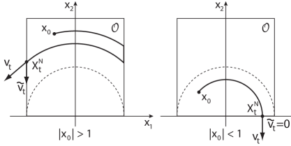
Figure 1.

∎

We next consider coupled reflected Brownian motion, for which we will need the following lemmas.

Lemma 6.2.

Suppose $\mathcal{O}$ is bounded and admissible. Then $\mathcal{O}\times\mathcal{O}$ is bounded and admissible as well. Furthermore, for each $(x,y)\in\partial(\mathcal{O}\times\mathcal{O})$, the set of normal vectors $\nu(x,y)$ defined by (2) has the representation

(34) $$\nu(x,y)=\left\{\left(\begin{array}[]{c}a_{1}\nu_{x}\\ a_{2}\nu_{y}\end{array}\right):\nu_{x}\in\nu(x),\nu_{y}\in\nu(y),a_{1}^{2}+a_{2}^{2}=1,a_{1},a_{2}>0\right\},\\ \text{ when }(x,y)\in\partial\mathcal{O}\times\partial\mathcal{O},$$

$$\nu(x,y)=\left\{\left(\begin{array}[]{c}\nu_{x}\\ 0\end{array}\right):\nu_{x}\in\nu(x)\right\},\text{ when }(x,y)\in\partial\mathcal{O}\times\mathcal{O},$$

and

$$\nu(x,y)=\left\{\left(\begin{array}[]{c}0\\ \nu_{y}\end{array}\right):\nu_{y}\in\nu(y)\right\},\text{ when }(x,y)\in\mathcal{O}\times\partial\mathcal{O}.$$

Proof.

The representation formulae are a straightforward consequence of the definition of inward pointing unit proximal normal vectors in (2). That $\mathcal{O}\times\mathcal{O}$ satisfies Part 1 of Definition 1.1 follows from the representation formulae and the fact that $\mathcal{O}$ satisfies Part 1 of Definition 1.1.

We next show that $\mathcal{O}\times\mathcal{O}$ satisfies Part 2 of Definition 1.1. Since $\mathcal{O}$ is bounded, $\phi$ is bounded in $\mathcal{O}$ and so after adding a constant to $\phi$ if necessary, we may assume that $\phi\geq 1$ in $\bar{\mathcal{O}}$.

Let $\Phi(x,y)\equiv\phi(x)\phi(y)$. Then for all $(x,y)\in\partial(\mathcal{O}\times\mathcal{O}),\quad\nu\in\nu(x,y)$, we have, by our representation formulae, that

$$\nabla\Phi(x,y)\cdot\nu= a_{1}\phi(y)\nabla\phi(x)\cdot\nu_{x}+a_{2}\phi(x)\nabla\phi(y)\cdot\nu_{y}$$

$$\geq a_{1}\phi(y)\alpha+a_{2}\phi(x)\alpha\geq\alpha(a_{1}+a_{2})\geq\alpha$$

(where $(a_{1},a_{2})=(1,0)$ and $(0,1)$ for the cases $(x,y)\in(\partial\mathcal{O}\times\mathcal{O})\cup(\mathcal{O}\times\partial\mathcal{O})$), and so Part 2 holds with the function $\Phi(x,y)$. Finally, as $\mathcal{O}\times\mathcal{O}$ is bounded, Part 3 follows immediately from Part 2. ∎

Lemma 6.3.

Let $\mathcal{O}$ be bounded and admissible. Then for $(x,y)\in\bar{\mathcal{O}}\times\bar{\mathcal{O}}$,

$$T_{\bar{\mathcal{O}}\times\bar{\mathcal{O}}}(x,y)=T_{\bar{\mathcal{O}}}(x)\times T_{\bar{\mathcal{O}}}(y).$$

Furthermore,

$$\text{{\rm proj}}_{T_{\bar{\mathcal{O}}\times\bar{\mathcal{O}}}(x,y)}\left(\begin{array}[]{c}\xi\\ \eta\end{array}\right)=\left(\begin{array}[]{c}\text{{\rm proj}}_{T_{\bar{\mathcal{O}}}(x)}(\xi)\\ \text{{\rm proj}}_{T_{\bar{\mathcal{O}}}(x)}(\eta)\end{array}\right)$$

Proof.

When $D\subset\mathbb{R}^{d}$ is admissible, it follows from Part 3. of Lemma 2.5 that

$$T_{\bar{D}}(z)=\{v\in\mathbb{R}^{d}:\lim_{h\searrow 0}\frac{d_{\bar{D}}(z+hv)}{h}=0\}$$

(i.e. $\lim$ replaces $\liminf$). Since $\mathcal{O}$, and by Lemma 6.2, $\mathcal{O}\times\mathcal{O}$, are bounded and admissible, the first statement then follows immediately from the relation

$$d^{2}_{\bar{\mathcal{O}}\times\bar{\mathcal{O}}}\left(\left(\begin{array}[]{c}x\\ y\end{array}\right)+h\left(\begin{array}[]{c}v\\ w\end{array}\right)\right)=d^{2}_{\bar{\mathcal{O}}}(x+hv)+d^{2}_{\bar{\mathcal{O}}}(y+hw).$$

The second statement then follows from the first by a similar argument. ∎

6.1. Synchronously Coupled Reflected Brownian Motion

We now discuss synchronously coupled reflected Brownian motion. A $d$-dimensional synchronously coupled reflected Brownian motion is a $2d$-dimensional process $Z_{t}=(X_{t},Y_{t})$ in a product domain $\bar{\mathcal{O}}\times\bar{\mathcal{O}}$ which satisfies the reflected SDE

$$dZ_{t}=\sigma(Z_{t})dW_{t}+dL_{t},$$

where

$$\sigma(z)\equiv\left(\begin{array}[]{c}I\\ I\end{array}\right).$$

Note that, because $\sigma$ is constant, there is no difference between the Stratonovich and Itô versions of the above SDE. We will express this reflected SDE in a more convenient form as the pair of reflected SDEs

$$dX_{t}=dW_{t}+dL_{t},\quad X_{0}=x_{0}\quad\text{and}\quad dY_{t}=dW_{t}+dM_{t},\quad Y_{0}=y_{0}.$$

We think of $X_{t}$ and $Y_{t}$ as being two $d$-dimensional processes which are driven by the same Brownian motion $W_{t}$ and which are constrained to lie in the same domain $\bar{\mathcal{O}}$. The two processes move in sync except for when one or the other is bumps against the boundary and gets nudged.

We now consider the geometric properties of synchronously coupled reflected Brownian motion in two domains. Such properties were used to prove the “hot spots conjecture” for these domains (See [2] and  [1] for more details).

Example 6.4.

Let $\mathcal{O}\subset\mathbb{R}^{2}$ be the obtuse triangle lying with its longest face on the horizontal axis, and denote its left and right acute angles by $\alpha$ and $\beta$. Suppose $x_{0}\neq y_{0}$, and for $x\neq y$, let $\angle(x,y)=\arg(y-x)$. Then, ${\mathbb{P}}$-almost surely,

(35) $$-\beta\leq\angle(x_{0},y_{0})\leq\alpha\implies\text{ for all $t$ either }-\beta\leq\angle(X_{t},Y_{t})\leq\alpha\text{ or }X_{t}=Y_{t}.$$

Proof.

By (31), it suffices to show that (35) holds ${\mathbb{P}}^{N}$-a.s. Fix $N$ and $W_{t}\in\Omega$. In view of Theorem 2.3 and Lemma 6.3 it will suffice to show that $X^{N}_{t}$ and $Y^{N}_{t}$ satisfy (35) where $X^{N}_{t}$ and $Y^{N}_{t}$ satisfy the ODE

(36) $$\begin{split}\dot{X}^{N}_{t}=&\text{{\rm proj}}_{T_{\bar{\mathcal{O}}}(X^{N}_{t})}(\dot{W}^{N}_{t}),\quad X^{N}_{0}=x_{0}\\ \dot{Y}^{N}_{t}=&\text{{\rm proj}}_{T_{\bar{\mathcal{O}}}(Y^{N}_{t})}(\dot{W}^{N}_{t}),\quad Y^{N}_{0}=y_{0}\end{split}$$

It is straightforward to check that the functions $X^{N}_{t}$, $Y^{N}_{t}$ starting at $X^{N}_{0}=x_{0}$, $Y^{N}_{0}=y_{0}$ and defined inductively for $t\in[m2^{-N},(m+1)2^{-N}]$ by $X^{N}_{t}=\text{{\rm proj}}_{\bar{\mathcal{O}}}(X^{N}_{m2^{-N}}+(t-m2^{-N})\dot{W}^{N}_{t})$ and $Y^{N}_{t}=\text{{\rm proj}}_{\bar{\mathcal{O}}}(Y^{N}_{m2^{-N}}+(t-m2^{-N})\dot{W}^{N}_{t})$ satisfy (36). A simple geometric argument shows that if $\angle(x,y)\in[-\beta,\alpha]$ then $\angle(\text{{\rm proj}}_{\bar{\mathcal{O}}}(x),\text{{\rm proj}}_{\bar{\mathcal{O}}}(y))\in[-\beta,\alpha]$ or $\text{{\rm proj}}_{\bar{\mathcal{O}}}(x)=\text{{\rm proj}}_{\bar{\mathcal{O}}}(y)$. From this it follows by induction that $X^{N}_{t}$ and $Y^{N}_{t}$ satisfy (35) as desired. Figure 2 shows a pair of sample paths $X^{N}_{t}$ and $Y^{N}_{t}$ in the interval $m2^{-N}\leq t\leq(m+1)2^{-N}$ where we use $v$ to denote the constant vector $2^{N}(W_{(m+1)2^{-N}}-W_{m2^{-N}})$. ∎

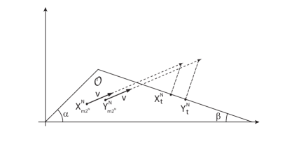
Figure 2.

Example 6.5.

(Proposition 2 in  [1])We now consider synchronously coupled reflected Brownian motion in a Lip domain. A lip domain is a domain in $\mathbb{R}^{2}$ which is bounded below by a function $f_{1}(x)$ and above by another function $f_{2}(x)$ each of which is Lipschitz continuous with constant bounded by $1$. The domains are so named because they look like a pair of lips (See Figure 3).

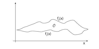
Figure 3.

Consider synchronously coupled reflected Brownian motion in a lip domain $\mathcal{O}$ where the defining functions $f_{1}(x)$ and $f_{2}(x)$ are smooth and have Lipschitz constants bounded by $\lambda<1$. Then $\mathcal{O}$ is a bounded admissible domain. Recall the definition of $\angle(x,y)$ from the previous example, and let $x_{0},y_{0}\in\mathbb{R}^{2}$ be such that $x_{0}\neq y_{0}$ and $\angle(x_{0},y_{0})\in[-\frac{\pi}{4},\frac{\pi}{4}]$. We have the following geometric property for the paths $X_{t}$ and $Y_{t}$:

(37) $$\forall t,\text{ either }\angle(X_{t},Y_{t})\in[-\frac{\pi}{4},\frac{\pi}{4}]\text{ or }X_{t}=Y_{t}\quad{\mathbb{P}}\text{-a.s.}$$

Proof.

In view of (31) and Theorem 2.3 it suffices to show that for every $W_{t}\in\Omega$, $X^{N}_{t}$ and $Y^{N}_{t}$ satisfy (37) when $X^{N}_{t}$ and $Y^{N}_{t}$ solve the ODE (36). Let $\Theta^{N}_{t}\equiv\angle(X^{N}_{t},Y^{N}_{t})$ or $0$ according to whether $X^{N}_{t}\neq Y^{N}_{t}$ or $X^{N}_{t}=Y^{N}_{t}$. It is enough to show that, $dt$-almost everywhere, $\dot{\Theta}^{N}_{t}\leq 0$ when $\Theta^{N}_{t}\in[\frac{\pi}{4},\frac{\pi}{2}-\tan^{-1}(\lambda)]$ and $\dot{\Theta}^{N}_{t}\geq 0$ when $-\Theta^{N}_{t}\in[\frac{\pi}{4},\frac{\pi}{2}-\tan^{-1}(\lambda)]$. By symmetry it will suffice to prove the first statement.

Let $v_{t}=\dot{W}^{N}_{t}$, $\tilde{v}_{t}=\text{{\rm proj}}_{T_{\mathcal{O}}(X^{N}_{t})}(v_{t})$, and $\tilde{v}^{\prime}_{t}=\text{{\rm proj}}_{T_{\mathcal{O}}(Y^{N}_{t})}(v_{t})$. We compute:

$$\frac{d}{dt}\left[\Theta^{N}_{t}\right]= \frac{d}{dt}\tan^{-1}\left(\frac{(Y^{N}_{t}-X^{N}_{t})_{2}}{(Y^{N}_{t}-X^{N}_{t})_{1}}\right)=\frac{(Y^{N}_{t}-X^{N}_{t})\cdot R(\tilde{v}_{t}-\tilde{v}^{\prime}_{t})}{|Y^{N}_{t}-X^{N}_{t}|^{2}}$$

$$= \frac{(Y^{N}_{t}-X^{N}_{t})\cdot R(\tilde{v}_{t}-v_{t})}{|Y^{N}_{t}-X^{N}_{t}|^{2}}+\frac{(Y^{N}_{t}-X^{N}_{t})\cdot R(v_{t}-\tilde{v}^{\prime}_{t})}{|Y^{N}_{t}-X^{N}_{t}|^{2}}$$

where $R=\left(\begin{array}[]{cc}0&-1\\ 1&0\end{array}\right)$ is the matrix which rotates vectors in $\mathbb{R}^{2}$ by $90^{\circ}$ counter-clockwise. Suppose $\Theta^{N}_{t}\in[\frac{\pi}{4},\frac{\pi}{2}-\tan^{-1}(\lambda)]$. Then since the Lipschitz constants of $f_{1}$ and $f_{2}$ are strictly less than $1$, $X^{N}_{t}$ cannot be on the $f_{2}$-boundary and $Y^{N}_{t}$ cannot be on the $f_{1}$-boundary. For each $t$, it follows that either $v_{t}=\tilde{v}_{t}$ or $\arg(R(\tilde{v}_{t}-v_{t}))\in[\pi-\tan^{-1}(\lambda),\pi+\tan^{-1}(\lambda)]$ and either $v_{t}=\tilde{v}^{\prime}_{t}$ or $\arg(R(v_{t}-\tilde{v}^{\prime}_{t}))\in[\pi-\tan^{-1}(\lambda),\pi+\tan^{-1}(\lambda)]$. And so each of the terms in the sum above is $\leq 0$. We depict in Figure 4 the case where $X^{N}_{t}\in\mathcal{O}$ and $Y^{N}_{t}\in\partial\mathcal{O}$.

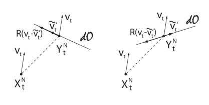
Figure 4.

∎

6.2. Mirror Coupled Reflected Brownian Motion

Our final example involves mirror coupled reflected Brownian motion. A $d$-dimensional mirror coupled reflected Brownian motion is a $2d$-dimensional process $Z_{t}=(X_{t},Y_{t})$ in a product domain $\bar{\mathcal{O}}\times\bar{\mathcal{O}}$ which satisfies the reflected SDE

(38) $$dZ_{t}=\sigma(Z_{t})dW_{t}+dL_{t},$$

where

$$\sigma(z)=\sigma(x,y)\equiv\left(\begin{array}[]{c}I\\ I-2\frac{(y-x)(y-x)^{\top}}{|y-x|^{2}}\end{array}\right),$$

defined up until the first time $\tau$ that $Z_{t}$ hits the diagonal of $\bar{\mathcal{O}}\times\bar{\mathcal{O}}$, at which point we stop our process (i.e. $Z_{t}\equiv Z_{\tau}$ for $t\geq\tau$). We will express this reflected SDE in a more convenient form as the pair of reflected SDEs

(39) $$\begin{split}dX_{t}=&dW_{t}+dL_{t},\quad X_{0}=x_{0}\\ dY_{t}=&(I-2\frac{(Y_{t}-X_{t})(Y_{t}-X_{t})^{\top}}{|Y_{t}-X_{t}|^{2}})dW_{t}+dM_{t},\quad Y_{0}=y_{0}.\end{split}$$

We think of $X_{t}$ and $Y_{t}$ as being two $d$-dimensional processes which are “mirror coupled” with respect to the driving Brownian motion $W_{t}$ and which are constrained to lie in the same domain $\bar{\mathcal{O}}$. That is, if you consider the hyperplane which perpendicularly bisects the line segment connecting $X_{t}$ and $Y_{t}$ to be a “mirror”, then the two processes move in such a way that they are mirror images of each other until either process bumps into the boundary and is nudged (which causes the mirror to shift). We refer the reader to the papers [2] and [1] for a more thorough overview.

We will prove the same geometric property we considered for synchronously coupled reflected Brownian motion in Example 6.5, but now for mirror coupled reflected Brownian motion. The point is that (38) can be viewed as a Stratonovich reflected SDE and so again it suffices to prove the geometric property for the approximating processes.

We make this rigorous with the following lemma which shows that, off of the diagonal of $\mathcal{O}\times\mathcal{O}$, the Stratonovich correction factor for (38) is $0$.

Lemma 6.6.

For $t<\tau$,

(40) $$\sum_{j=1}^{d}\frac{1}{2}d\left<\left(I-2\frac{(Y_{t}-X_{t})(Y_{t}-X_{t})^{\top}}{|Y_{t}-X_{t}|^{2}}\right)_{ij},(W_{t})_{j}\right>=0$$

In fact,

(41) $$d\left<\left(I-2\frac{(Y_{t}-X_{t})(Y_{t}-X_{t})^{\top}}{|Y_{t}-X_{t}|^{2}}\right)_{ij},(W_{t})_{j}\right>=0,\text{ for each }j$$

Proof.

It suffices to prove (41). Let $V_{i}\equiv(Y_{t}-X_{t})_{i}$, where we have suppressed the dependence of $V_{i}$ on $t$. An easy calculation shows that

$$d\langle V_{\ell},(W_{t})_{j}\rangle=\frac{-2V_{j}V_{\ell}}{\sum_{k}V_{k}^{2}}dt$$

and

$$\frac{\partial}{\partial V_{i}}\left(\frac{V_{i}V_{j}}{\sum_{k}V_{k}^{2}}\right)= \frac{V_{j}(\sum_{k}V_{k}^{2})-2V_{i}^{2}V_{j}}{(\sum_{k}V_{k}^{2})^{2}}$$

$$\frac{\partial}{\partial V_{j}}\left(\frac{V_{i}V_{j}}{\sum_{k}V_{k}^{2}}\right)= \frac{V_{i}(\sum_{k}V_{k}^{2})-2V_{i}V_{j}^{2}}{(\sum_{k}V_{k}^{2})^{2}}$$

$$\frac{\partial}{\partial V_{\ell}}\left(\frac{V_{i}V_{j}}{\sum_{k}V_{k}^{2}}\right)= \frac{-2V_{i}V_{j}V_{\ell}}{(\sum_{k}V_{k}^{2})^{2}},\text{ for }\ell\neq i,j$$

Putting these together, we have that

$$d\langle\frac{V_{i}V_{j}}{\sum_{k}V_{k}^{2}},(W_{t})_{j}\rangle= \left(\frac{V_{j}(\sum_{k}V_{k}^{2})-2V_{i}^{2}V_{j}}{(\sum_{k}V_{k}^{2})^{2}}\right)\left(\frac{-2V_{j}V_{i}}{\sum_{k}V_{k}^{2}}\right)$$

$$+\left(\frac{V_{i}(\sum_{k}V_{k}^{2})-2V_{i}V_{j}^{2}}{(\sum_{k}V_{k}^{2})^{2}}\right)\left(\frac{-2V_{j}^{2}}{\sum_{k}V_{k}^{2}}\right)$$

$$+\sum_{\ell\neq i,j}\left(\frac{-2V_{i}V_{j}V_{\ell}}{(\sum_{k}V_{k}^{2})^{2}}\right)\left(\frac{-2V_{j}V_{\ell}}{\sum_{k}V_{k}^{2}}\right)=0$$

From this, (41) immediately follows.

∎

We now prove a geometric property.

Example 6.7.

(Example 6.5 for mirror coupling) Let $\mathcal{O}$ be the same lip domain defined by smooth functions considered in Example 6.5 and consider the mirror coupled reflected Brownian motion starting from $x_{0}$ and $y_{0}$ where $x_{0}\neq y_{0}$. Then (37) holds where where $X_{t}$ and $Y_{t}$ are given by (39).

Proof.

Let $D_{\varepsilon}=\{z=(x,y)\in\bar{\mathcal{O}}\times\bar{\mathcal{O}}:|x-y|<\varepsilon\}$ be the “$\varepsilon$-diagonal” of $\bar{\mathcal{O}}\times\bar{\mathcal{O}}$. Consider a sequence of smooth functions $\rho_{k}:\bar{\mathcal{O}}\times\bar{\mathcal{O}}\rightarrow[0,1]$ such that $\rho(z)\equiv 0$ on $D_{\frac{1}{2k}}$ and $\rho(z)\equiv 1$ off of $D_{\frac{1}{k}}$. Let $\sigma_{k}(z)=\rho_{k}(z)\sigma(z)$. Then $\sigma_{k}\in C^{2}(\bar{\mathcal{O}}\times\bar{\mathcal{O}})$.

Let ${\mathbb{P}}^{k}$ be the measure on $Z$-pathspace induced by the solutions to the reflected SDE

$$dZ^{k}_{t}=\sigma_{k}(Z^{k}_{t})\circ dW_{t}+dL^{k}_{t}$$

and define ${\mathbb{P}}^{k,N}$ to be the measures on $Z$-pathspace induced by solutions to the approximating reflected ODE

(42) $$dZ^{k,N}_{t}=\sigma_{k}(Z^{k,N}_{t})dW^{N}_{t}+dL^{k,N}_{t}$$

Recall that the stopping time $\tau$ corresponds to the first time $X_{t}$ equals $Y_{t}$ and define $\tau_{k}\equiv\inf\{t:|X_{t}-Y_{t}|<\frac{1}{k}\}$. Let $S=\{Z_{t}\in C([0,\infty);\mathbb{R}^{2d}):-\frac{\pi}{4}\leq\angle(X_{t},Y_{t})\leq\frac{\pi}{4},\forall t<\tau\}$ and let $S_{k}=\{Z_{t}\in C([0,\infty);\mathbb{R}^{2d}):-\frac{\pi}{4}\leq\angle(X_{t},Y_{t})\leq\frac{\pi}{4},\forall t<\tau_{k}\}$.

Our goal is to show that ${\mathbb{P}}(S)=1$, where ${\mathbb{P}}$ is the measure induced on $Z$-pathspace by (38). It is clear that the subsets $S_{k}$ decrease monotonically to $S$, and so it suffices to prove that ${\mathbb{P}}(S_{k})=1,\forall k$.

We first claim that ${\mathbb{P}}(S_{k})={\mathbb{P}}^{k}(S_{k})$. This is true because $S_{k}$ is $\mathcal{F}_{\tau_{k}}$-measurable, and, in view of Lemma 6.6 and the equality $\sigma=\sigma_{k}$ on $D_{\frac{1}{k}}$, it is clear that ${\mathbb{P}}(A)={\mathbb{P}}^{k}(A)$ for $A\in\mathcal{F}_{\tau_{k}}$. So we need only show that ${\mathbb{P}}^{k}(S_{k})=1$, and for this it will suffice to show that ${\mathbb{P}}^{k,N}(S_{k})=1$. We argue this as we did in Example 6.5.

Fix $N$ and $W_{t}\in\Omega$ and let $\Theta^{k,N}_{t}\equiv\angle(X^{k,N}_{t},Y^{k,N}_{t})$. By symmetry, it is enough to show that $\dot{\Theta}^{k,N}_{t}\leq 0$ for $\Theta^{k,N}_{t}\in[\frac{\pi}{4},\frac{\pi}{2}-\tan^{-1}(\lambda)]$ for almost every $t<\tau_{k}$. Let $v_{t}=\dot{W}^{N}_{t}$ and

$$w_{t}=\left(I-\frac{(Y^{k,N}_{t}-X^{k,N}_{t})(Y^{k,N}_{t}-X^{k,N}_{t})^{\top}}{|Y^{k,N}_{t}-X^{k,N}_{t}|^{2}}\right)v_{t},$$

Then, in view of Theorem 2.3 and Lemma 6.3, $\dot{X}^{k,N}_{t}=\tilde{v}_{t}\equiv\text{{\rm proj}}_{T_{\bar{\mathcal{O}}}(X^{N}_{t})}(v_{t})$ and $\dot{Y}^{k,N}_{t}=\tilde{w}_{t}\equiv\text{{\rm proj}}_{T_{\bar{\mathcal{O}}}(Y^{N}_{t})}(w_{t})$ (recall that $\rho_{k}(X^{k,N}_{t},Y^{k,N}_{t})=1$ for $t<\tau_{k}$).

We compute:

$$\dot{\Theta}^{k,N}_{t}= \frac{(Y^{N,k}_{t}-X^{N,k}_{t})\cdot R(\tilde{v}_{t}-\tilde{w}_{t})}{|Y^{N,k}_{t}-X^{N,k}_{t}|^{2}}$$

$$= \frac{(Y^{N,k}_{t}-X^{N,k}_{t})\cdot R(\tilde{v}_{t}-v_{t})}{|Y^{N,k}_{t}-X^{N,k}_{t}|^{2}}+\frac{(Y^{N,k}_{t}-X^{N,k}_{t})\cdot R(v_{t}-w_{t})}{|Y^{N,k}_{t}-X^{N,k}_{t}|^{2}}$$

$$+\frac{(Y^{N,k}_{t}-X^{N,k}_{t})\cdot R(w_{t}-\tilde{w}_{t})}{|Y^{N,k}_{t}-X^{N,k}_{t}|^{2}}$$

The argument in the Proof 6.1 again shows that the first and third terms are non-positive. That the second term is non-positive follows from the fact that either $v_{t}=w_{t}$ or $\arg(v_{t}-w_{t})=\pm\Theta^{k,N}_{t}$. ∎

References

[1]
Rami Atar and Krzysztof Burdzy.
On Neumann eigenfunctions in lip domains.
J. Amer. Math. Soc., 17(2):243–265 (electronic), 2004.
[2]
Rodrigo Bañuelos and Krzysztof Burdzy.
On the “hot spots” conjecture of J. Rauch.
J. Funct. Anal., 164(1):1–33, 1999.
[3]
Piernicola Bettiol.
A deterministic approach to the Skorokhod problem.
Control Cybernet., 35(4):787–802, 2006.
[4]
Bernard Cornet.
Existence of slow solutions for a class of differential inclusions.
J. Math. Anal. Appl., 96(1):130–147, 1983.
[5]
Arturo Kohatsu-Higa.
Stratonovich type SDE’s with normal reflection driven by
semimartingales.
Sankhyā Ser. A, 63(2):194–228, 2001.
[6]
P.-L. Lions and A.-S. Sznitman.
Stochastic differential equations with reflecting boundary
conditions.
Comm. Pure Appl. Math., 37(4):511–537, 1984.
[7]
Roger Petterson.
Wong-zakai approximations for reflecting stochastic differential
equations.
Stochastic Analysis and Applications, 17(4):609–617, 1999.
[8]
R. A. Poliquin, R. T. Rockafellar, and L. Thibault.
Local differentiability of distance functions.
Trans. Amer. Math. Soc., 352(11):5231–5249, 2000.
[9]
R. Tyrrell Rockafellar and Roger J.-B. Wets.
Variational analysis, volume 317 of Grundlehren der
Mathematischen Wissenschaften [Fundamental Principles of Mathematical
Sciences].
Springer-Verlag, Berlin, 1998.
[10]
Yasumasa Saisho.
Stochastic differential equations for multidimensional domain with
reflecting boundary.
Probab. Theory Related Fields, 74(3):455–477, 1987.
[11]
Daniel W. Stroock and S. R. S. Varadhan.
Diffusion processes with boundary conditions.
Comm. Pure Appl. Math., 24:147–225, 1971.
[12]
Hiroshi Tanaka.
Stochastic differential equations with reflecting boundary condition
in convex regions.
Hiroshima Math. J., 9(1):163–177, 1979.
[13]
Richard Vinter.
Optimal control.
Systems & Control: Foundations & Applications. Birkhäuser Boston
Inc., Boston, MA, 2000.
[14]
Eugene Wong and Moshe Zakai.
On the convergence of ordinary integrals to stochastic integrals.
Ann. Math. Statist., 36:1560–1564, 1965.