Modulational instability of ion-acoustic wave packets in quantum pair-ion plasmas

Abstract

Amplitude modulation of quantum ion-acoustic waves (QIAWs) in a quantum electron-pair-ion plasma is studied. It is shown that the quantum coupling parameter $H$ (being the ratio of the plasmonic energy density to the Fermi energy) is ultimate responsible for the modulational stability of QIAW packets, without which the wave becomes modulational unstable. New regimes for the modulational stability (MS) and instability (MI) are obtained in terms of $\ H$ and the positive to negative ion density ratio $\beta.$ The growth rate of MI is obtained, the maximum value of which increases with $\beta$ and decreases with $H$. The results could be important for understanding the origin of modulated QIAW packets in the environments of dense astrophysical objects, laboratory negative ion plasmas as well as for the next generation laser solid density plasma experiments.

LABEL:FirstPage1 LABEL:LastPage#1102

In the recent years, there has been a growing interest in investigating various collective modes and their properties in pair-ion plasmas (see, e.g., Refs. Hasegawa ; Cramer ; Misra1 ; Samanta ).  Such plasmas are believed to be ubiquitous in most space and laboratory plasmas Amemiya ; Franklin . Moreover, it has been investigated that the pair-ion plasmas have potential applications in the atmosphere of D-region of Earth’s ionosphere, Earth’s mesosphere, the solar atmosphere, as well as in the microelectronic plasma processing reactors Kim . Recent investigations indicate that such pair-ion plasmas could also be important with regard to the diagnostic point of view, since the dispersion properties of wave modes can be used to deduce the plasma parameters Samanta . On the other hand, in view of wide applications in dense astrophysical environments as well as in intense laser produced plasmas, Misra studied the formation of ion-acoustic shock-like oscillations in quantum pair-ion plasmas Misra1 . Again, the propagation of wave packets in a dispersive nonlinear plasma medium (where the dispersion is due to quantum tunneling associated with the Bohm potential) has been known to be subjected to the amplitude modulation, i.e., a slow variation of the wave packet’s envelope due to nonlinearity. The system’s evolution is then governed through the modulational instability (MI). A number of works can be found in the literature to study the MI in various quantum plasma systems (e.g., see Refs. Misra2 ; Sabry ; Misra3 ).

In this work, we study the important effect of quantum tunneling associated with the Bohm potential on the MI of quantum ion-acoustic waves (QIAWs) in an electron-pair-ion plasma. We show that the quantum coupling parameter $H$ is ultimate responsible for the stability of modulated QIAW packets, without which the wave becomes modulational unstable. New regimes for the MI are obtained with the variation of $H$ along with the positive to negative ion density ratio $\beta.$ We also obtain the growth rate of MI in terms of the system parameters.

In what follows, we consider the nonlinear propagation of QIAWs in an ummagnetized quantum plasma composed of electrons and both positive and negative ions. The basic normalized equations read Misra1

$$\phi=-\frac{1}{2}+\frac{1}{2}{n_{e}^{2/3}}-\frac{H^{2}}{2\mu}\frac{1}{\sqrt{n_{e}}}\frac{\partial^{2}\sqrt{n_{e}}}{\partial x^{2}},$$ (1)

$$\frac{\partial n_{\alpha}}{\partial t}+\frac{\partial(n_{\alpha}u_{\alpha})}{\partial x}=0,$$ (2)

$$\frac{\partial u_{\alpha}}{\partial t}+{u_{\alpha}}\frac{\partial{u_{\alpha}}}{\partial x}=-\varsigma_{\alpha}\frac{\partial\phi}{\partial x},$$ (3)

$$\frac{\partial^{2}\phi}{\partial x^{2}}={(\beta-1)n_{e}}-{\beta}{n_{+}}+{n_{-}},$$ (4)

where the suffix $\alpha=+,-$ indicate the quantities for positive and negative ions respectively. Also, $\phi$ is the electrostatic potential normalized by $k_{B}T_{Fe}/e$ with $k_{B}$ denoting the Boltzmann constant, $e$ the elementary charge and $T_{Fe}\equiv\hbar^{2}(3\pi^{2}n_{e0})^{2/3}/2k_{B}m_{e}$ the electron Fermi temperature. Here $\hbar$ is the Planck’s constant divided by $2\pi,$ $m_{e}$ is the electron mass and $n_{e0}$ is its equilibrium number density. Moreover, $n_{\alpha}$ denotes the $\alpha$-particle perturbed number density normalized by its equilibrium value $n_{\alpha 0},$ $H\equiv\hbar{\omega_{pe}/}k_{B}T_{Fe}$ is the nondimensional quantum parameter describing the ratio of the plasmonic energy density to the Fermi energy, $\omega_{p\alpha}\equiv\sqrt{n_{\alpha 0}e^{2}/\varepsilon_{0}m_{\alpha}}$ is the $\alpha$-particle plasma frequency and $m_{\alpha}$ is the mass. The speed of the $\alpha$-species particle $u_{\alpha}$ is  normalized by the quantum ion-acoustic speed $c_{s}\equiv\sqrt{k_{B}T_{Fe}/m_{-}},$ the space $(x)$ and time $(t)$ variables are normalized by $c_{s}/\omega_{p-}$ and $\omega_{p-}^{-1}$ respectively. In Eq. (3), $\varsigma_{(+,-)}=(m,-1)$ with $m\equiv Z_{+}m_{-}/Z_{-}m_{+}.$ The parameter $\beta=Z_{+}n_{+0}/Z_{-}n_{-0}$ appearing in Eq. (4) is the positive to negative ion density ratio with $Z_{+,-}$ denoting the positive (negative) ion charge states. The second term in the right-hand side of Eq. (1) is due to the three-dimensional (3D) Fermi-Dirac pressure law for electrons given by Landau ; Manfredi

$$p_{e}=\frac{1}{5}\frac{m_{e}V_{Fe}^{2}}{n_{e0}^{2/3}}n_{e}^{5/3}.$$ (5)

Since the equilibrium distribution is always 3D even in one-dimensional (1D) geometry (we can project the 3D Fermi-Dirac distribution over $x$-direction), the equilibrium pressure must indeed be given by its 3D expression [Eq. (5)] Manfredi .

In order to obtain an evolution equation describing the propagation of modulated QIAW envelopes we employ the standard reductive perturbation technique (RPT) in which the independent variables $x$ and $t$ are stretched as (see, e.g., Ref. Misra2 )$\ \xi$ $=\epsilon(x-v_{g}t)$ and $\tau=\epsilon^{2}t$, where $v_{g}$ (normalized by $c_{s}$) is the wave’s group velocity to be determined by the compatibility condition. The dependent variables (where the perturbed parts depend on the fast scales via the phase $kx-\omega t$, and the slow scales only enter the $l$-th harmonic amplitude) are expanded as

$$\left({n_{\alpha},u_{\alpha},\phi}\right) =\left(1,0,0\right)+\sum_{n=1}^{\infty}\epsilon^{n}\sum_{l=-\infty}^{\infty}\left[n_{\alpha l}^{(n)},u_{\alpha l}^{(n)},\phi_{\alpha l}^{(n)}\right]$$

$$\times\exp\left[i(kx-\omega t)l\right],$$ (6)

where $\omega,$ $k$ are the normalized wave frequency and wave number respectively. The state variables $n_{\alpha l}^{(n)}$, etc., satisfy the reality condition $A_{-l}^{(n)}=A_{l}^{(n)\ast}$ with asterisk denoting the complex conjugate. Now, substituting the expansion [Eq.(6)] into equations (1)-(4) and expressing the variables $x$ and $t$ in terms of the stretched coordinates $\xi$, $\tau$, and then collecting the terms in different power of $\epsilon$ we obtain for $n=1,l=1$ the first order quantities,

$$n_{e1}^{(1)}=\frac{\phi_{1}^{(1)}}{\Lambda},\text{ }n_{\alpha 1}^{(1)}=\frac{\varsigma_{\alpha}k^{2}}{\omega^{2}}\phi_{1}^{(1)},\text{ }u_{\alpha 1}^{(1)}=\frac{\varsigma_{\alpha}k}{\omega}\phi_{1}^{(1)},$$ (7)

and the following dispersion relation

$${\omega^{2}}=\frac{(1+\beta m){k^{2}}}{{k^{2}}+(\beta-1)/\Lambda},$$ (8)

where $\Lambda=1/3+H^{2}k^{2}/4(\beta-1).$ The dispersion relation modified by the density ratio $\beta$ as well as the quantum parameter $H$ gives two real eigen modes for the carrier waves. In particular, by disregarding the negative ion dynamics and considering one-dimensional Fermi pressure law one can recover the previous result dispersion . In the short-wavelength limit (or for large $k)$, the frequency of QIAWs approaches a constant value $\sqrt{1+\beta m},$ whereas for large wavelength, the frequency increases with $k$. The compatibility condition is obtained from the second order $(n=2)$ reduced equations with $l=1$ as

$${v_{g}}\equiv\frac{\partial\omega}{\partial k}=\frac{\omega}{k(1+{\beta m})}\left[(1+{\beta m})-{\omega^{2}}+\frac{H^{2}{\omega^{2}}}{{4}\Lambda^{2}}\right].$$ (9)

Proceeding in the same way as in Refs. Misra2 ; Misra3 and substituting all the above derived expressions from $n=2,l=2;n=2,l=0$ into the components for $n=3,l=1$ of the reduced equations we obtain the following Nonlinear Schrödinger equation (NLSE)

$$i\frac{\partial\phi}{\partial\tau}+P\frac{\partial^{2}\phi}{\partial\xi^{2}}+Q|\phi|^{2}\phi=0,$$ (10)

where $\phi\equiv\phi_{1}^{(1)}$ and the dispersive and nonlinear coefficients $P$, $Q$ are respectively given by

$${P} =\frac{1}{2k(1+\beta m)}\left[(1+\beta m)\left(v_{g}-\frac{\omega}{k}\right)-\omega^{2}\left({3v_{g}}-\frac{\omega}{k}\right)\right.$$

$$\left.+\frac{H^{2}\omega^{2}}{4\Lambda^{2}}\left(3v_{g}-\frac{\omega}{k\Lambda}\left(\frac{1}{3}+\frac{5{H^{2}k^{2}}}{{{4(\beta-1)}}}\right)\right)\right],$$ (11)

$$Q=\frac{\omega^{3}/2k^{2}}{(1+\beta m)}\left[\frac{1}{\Lambda^{2}}\left[({{\beta-1)\Delta}}_{1}-{{\Delta}}_{2}\right]-\frac{k^{2}}{\omega^{2}}\left(\frac{2k}{\omega}{{\Delta}}_{3}+{{\Delta}}_{4}\right)\right],$$ (12)

with

$${{\Delta}}_{1}=2(A+A_{0})+\frac{1}{9}\left(\frac{9H^{2}k^{2}}{4\mu}-5\right)(F+F_{0}),$$ (13)

$${{\Delta}}_{2}=\frac{1}{4}(2F+F_{0})+\frac{({{\beta-1)}}\left(7+81H^{2}k^{2}/4\mu\right)}{27\Lambda^{2}},$$ (14)

$${{\Delta}}_{3}=(D+D_{0})\beta m+(E+E_{0}),$$ (15)

$${{\Delta}}_{4}=(B+B_{0})\beta m+(C+C_{0}).$$ (16)

The coefficients $A,$ $B,...A_{0},$ $B_{0},...$etc., in Eqs. (11) and (12) are given in the Appendix A. Equation (10) describes the slow modulation of the first order plasma potential of QIAWs in an unmagnetized electron-pair-ion plasma. Neglecting the electron dynamics, one recovers ion-acoustic envelope solitons in a pair-ion plasma pairplasma . The dispersion coefficient $P\equiv\partial^{2}\omega/2\partial k^{2}$ arising due to quantum diffraction and the charge separation of the plasma particles, and the nonlinear coefficient $Q$, due to the carrier wave self-interaction, are significantly modified by the quantum effects, as well as by the presence of negative ions in our plasma system.

To study the MI of QIAW packets, we assume a monochromatic solution of Eq. (10) to be of the form $\phi=\phi_{0}$exp$(iQ|\phi_{0}|^{2}\tau)$ (see e.g., Refs. Misra2 ; Misra3 ), where $\phi_{0}$ is the constant amplitude of the carrier wave and $\Delta(\tau)=-Q|\phi_{0}|^{2}$ is the nonlinear frequency shift. The amplitude and the phase of this solution is modulated against the linear perturbations as $\phi=[\phi_{0}+\phi_{1}$cos$(K\xi-\Omega\tau)]$exp$\left[iQ|\phi_{0}|^{2}\tau+i\theta_{1}cos(K\xi-\Omega\tau)\right]$, where $K$ and $\Omega$ are, respectively, the wave number and the wave frequency of modulation. We then obtain from Eq. (10) the dispersion relation

$$\Omega=PK^{2}\sqrt{1-\frac{K_{c}^{2}}{K^{2}}},$$ (17)

where $K_{c}=\sqrt{2Q/P}|\Phi_{0}|$ is the critical value of $K$, such that the MI sets in for $K<K_{c}$, or for wavelengths above the threshold $\lambda_{c}=2\pi/K_{c}$. The instability growth rate (letting $\Omega=i\Gamma)$ is obtained as

$$\Gamma=PK^{2}\sqrt{\frac{K_{c}^{2}}{K^{2}}-1,}$$ (18)

Clearly, the maximum growth rate obtained at $K=K_{c}/\sqrt{2}$ is $\Gamma_{max}=|Q||\Phi|^{2}$.

It is evident from Eq. (17) that the instability condition depends only on the sign of the product $PQ$. Also, relying on the positive or negative sign of $PQ$ one can predict that when $PQ>0$ the monochromatic waves become modulationally unstable leading to the formation of a bright soliton, i.e. a localized pulse-like envelope modulating the carrier wave. When $P/Q<0$, the solution is modulationally stable, which may result to the formation of a dark or grey soliton, representing a localized region of decreased amplitude. Thus, it is reasonable to study the behaviors of $PQ$ , which can be done numerically with the variation of the system parameters, namely, the density ratio $\beta$ and the quantum coupling parameter $H$. This is the main purpose of our present work.

We have considered the density ratio $\beta$ to be greater than unity and the range of values of $H<1$ for which the electron Fermi speed $v_{F}\equiv\sqrt{2k_{B}T_{Fe}/m_{e}}$ $<<c$, the speed of light in vacuum and the quantum collective, mean-field effects become important (where the quantum coupling parameter $g_{Q}\sim(n_{e0}\lambda_{F}^{3})^{-2/3}\lesssim 1,$ where $\lambda_{F}$ describes the scale length for electrostatic screening$)$. The variations of $P/Q$ with respect to $k$ for different values of $H$ (with fixed $m$ and $\beta)$ and for different $\beta$ (with fixed $m$ and $H)$ are shown graphically in Figs. 1 and 2 respectively. When $\beta=4$, i.e., when the electron concentration is $3/4$ times that of the positive ion, the stability $(PQ<0)$ and instability $(PQ>0)$ regions (see Fig. 1) for $H=0.75$ and $H=0.7$ are respectively $0<k<0.726;$ $k\gtrsim 0.726$ and $0<k<0.4982;$ $k\gtrsim 0.4982$.

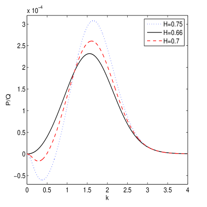
Figure 1: (Color online) $P/Q$ is plotted against $k$ to show the stable $(P/Q<0)$ and unstable $(P/Q>0)$ regions for $\beta=4$, $m=4$ and for different values of $H$: $H=0.66$ (solid line), $H=0.7$ (dashed line) and $H=0.75$ (dotted line). The details given in the text.

We find from Fig. 1 that for $H\leq 0.66,$ $PQ$ becomes positive for all values of $k$ and any $\beta$. The stability region decreases with decreasing the values of $H$. Thus, decreasing the values of $H$ or entering into the density region $n_{e0}\sim 1.3490\times 10^{31}$m^-3 or higher, one can find unstable modulated QIAWs.

We note that in order to observe different stable and unstable regions for higher values of $H$ $\geq 0.75$ we must have to increase the $\beta$-values as well to satisfy the restriction for quantum coupling parameter $g_{Q}$ as described above. Upon increasing the values of the density ratio $\beta$ keeping $H=0.7$ fixed, one can find significant change of the stable as well as unstable regions. These can be seen from Fig. 2. In this figure, for $\beta=5,$ $PQ$ is negative in $0<k<0.5755$ and positive otherwise,  whereas for $\beta=6,$ $PQ<0$ in $0<k<0.64$ and $PQ>0$ otherwise. Thus, fixing the electron concentration, and decreasing the positive ion concentration we can recover the stable regions in a larger domain of $k$.

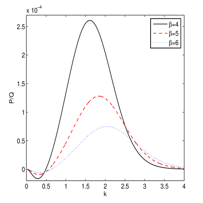
Figure 2: (Color online) The same as in Fig. 1, but for $H=0.7$, $m=4$ and for different values of $\beta$: $\beta=4$ (solid line), $\beta=5$ (dashed line) and $\beta=6$ (dotted line). The details given in the text.

We find that both the dark or grey ($PQ<0$) and the bright $(PQ>0)$ soliton excitations  are possible in our quantum plasma system. In the long-wavelength run $(k<1)$, the former dominates over a long range of values of $k$ (for a fixed $H$ and increasing $\beta)$, while the latter exists in a bounded short-range of $k$.

It is to be added that if in any case the plasma system contains negatively charged dust grains as impurities in the background, one can simply replace $\beta$ by $\beta-\delta$, where $\delta$ represents the percentage of negatively charged dust grains with respect to the negative ion concentration. In presence of negative dusts we may observe that for a fixed $H=0.7,m=4=\beta,$ $PQ<0$ in $0<k<0.5505$ and positive otherwise for $\delta=0.2,$and for $\delta=0.4,$ $PQ<0$ in $0<k<0.464$ and positive otherwise. This is how the charged dust impurity can modify the MI domains.  Changing $m$ does not modify the stability or instability regions, but the magnitudes of $P/Q,$ which can be important for calculating soliton widths at different parameters. The growth rate of MI is also calculated. It is seen that the absolute value of the maximum growth rate as well as the critical wave number increases (decreases) with increasing the $\beta$ ($H$) values.

To summarize, we have investigated the instability criteria for the amplitude modulation of QIAWs in a quantum pair-ion plasma. The quantum coupling parameter $H$ is shown to play crucial roles in stabilizing the QIAW packets. New regimes for the MI with the system parameters $H$ and $\beta$ are obtained in the domain of carrier wave numbers. The results could be important for negative ion plasmas, forthcoming laser produced plasmas in the laboratory as well as in dense astrophysical environments.

Acknowledgements

A. P. M.  gratefully acknowledges support from the Kempe Foundations, Sweden.

APPENDIX A

The coefficients appearing in Eqs. (11) and (12) are given as follows

$${A} =\left[\frac{3k^{4}(1-\beta m^{2})}{2\omega^{4}}+{\mu}\left({\frac{1}{18}+{\frac{3H^{2}k^{2}}{8\mu}}}\right)\right]$$

$$\times\left[\frac{k^{2}(1+{}\beta m-{4\omega^{2}})}{\omega^{2}}-\frac{\mu}{\left(1/3+{H^{2}k^{2}/{4\mu}}\right)}\right]^{-1},\text{ }$$

$${B}=\frac{mk^{2}}{\omega^{2}}\left(A+\frac{3mk^{2}}{2\omega^{2}}\right),\text{ }{C}=\frac{k^{2}}{\omega}\left(-A+\frac{3k^{2}}{2\omega^{2}}\right),$$

$${D}=\frac{mk}{\omega}\left(A+\frac{mk^{2}}{2\omega^{2}}\right),\text{ }{E}=\frac{k}{\omega}\left(-A+\frac{k^{2}}{2\omega^{2}}\right),\text{ }$$

$${F}=\frac{1}{\left(1/3+H^{2}k^{2}/{\mu}\right)}\left[A+\left(\frac{1}{18}+\frac{3H^{2}k^{2}}{8\mu}\right)/\left(\frac{1}{3}+\frac{H^{2}k^{2}}{4\mu}\right)^{2}\right],$$

$${A_{0}} =\frac{(m^{2}\beta-1){k^{2}}}{v_{g}\omega^{2}}\left(\frac{2k}{\omega}+\frac{1}{v_{g}}\right)-\frac{\left(9H^{2}k^{2}-32\mu/3\right)}{4\left(1/3+H^{2}k^{2}/4\mu\right)^{2}},$$

$${B_{0}} =\left[\frac{m^{2}k^{2}}{v_{g}\omega^{2}}\left(\frac{1}{v_{g}}+\frac{2k}{\omega}\right)+\frac{A_{0}m}{v_{g}^{2}}\right],$$

,

$${C_{0}} =\left[\frac{k^{2}}{v_{g}\omega^{2}}\left(\frac{1}{v_{g}}+\frac{2k}{\omega}\right)-\frac{A_{0}}{v_{g}^{2}}\right],\text{ }{D_{0}}=\left[\frac{m}{v_{g}}\left(A_{0}+\frac{mk^{2}}{\omega^{2}}\right)\right],\text{ }$$

$${E_{0}} =\left[\frac{1}{v_{g}}\left(-A_{0}+\frac{k^{2}}{\omega^{2}}\right)\right],{F_{0}}=\left[A_{0}+\frac{\left(9H^{2}k^{2}-32\mu/3\right)}{4\mu\left(1/3+H^{2}k^{2}/4\mu\right)^{2}}\right].$$

References

- (1) A. Hasegawa and P. K. Shukla, Phys. Scr., T116, 105 (2005).
- (2) N. F. Cramer and G. -M. Yung, Plasma Phys. Control. Fusion 28, 1043 (1986).
- (3) A. P. Misra, Phys. Plasmas 16, 033702 (2009).
- (4) S. Samanta and A. P. Misra, Phys. Plasmas 16, 074505 (2009).
- (5) H. Amemiya, B. M. Annaratone, and J. E. Allen, Plasma Sources Sci. Technol. 8, 179 (1999).
- (6) R. N. Franklin, Plasma Sources Sci. Technol. 11, A31 (2002).
- (7) S. H. Kim and R. L. Merlino, Phys. Rev. E 76, 035401 (2007).
- (8) A. P. Misra and P. K. Shukla, Phys. Plasmas 14, 082312 (2007); 15, 122107 (2008); 15, 052105 (2008).
- (9) R. Sabry, W. M. Moslem, and P. K. Shukla Eur. Phys. J. D 51, 233 (2009).
- (10) A. P. Misra, C. Bhowmik, and P. K. Shukla, Phys. Plasmas 16, 072116 (2009).
- (11) L. D. Landau and E. M. Lifshitz, Statistical Physics (Oxford University Press, Oxford, 1980), Pt. 1, p.167; G. Manfredi and F. Haas, Phys. Rev. B 64, 075316 (2001).
- (12) G. Manfredi, Fields Inst. Commun. 46, 263 (2005).
- (13) F. Haas, L. G. Garcia, J. Goedert, and G. Manfredi, Phys. Plasmas 10, 3858 (2003).
- (14) R. Sabry, Phys. Plasmas 15, 092101 (2008).