On critical collapse of gravitational waves

Abstract

An axisymmetric collapse of non-rotating gravitational waves is numerically investigated in the subcritical regime where no black holes form but where curvature attains a maximum and decreases, following the dispersion of the initial wave packet. We focus on a curvature invariant with dimensions of length, and find that near the threshold for black hole formation it reaches a maximum along concentric rings of finite radius around the axis. In this regime the maximal value of the invariant exhibits a power-law scaling with the approximate exponent 0.38, as a function of a parametric distance from the threshold. In addition, the variation of the curvature in the critical limit is accompanied by increasing amount of echos, with nearly equal temporal and spatial periods. The scaling and the echoing patterns, and the corresponding constants are independent of the initial data and coordinate choices.

1 Introduction

Universality, scaling and self-similarity found in critical gravitational collapse is one of the most fascinating phenomena associated with gravitational interactions. First discovered numerically by Choptuik [1] in spherically-symmetric collapse of massless scalar field, this distinctive behaviour was later observed in other systems, including those with various matter contents and equations of state, diverse spacetime dimensions etc. However, while a great deal of literature has emerged on critical phenomena in spherical symmetry, only a limited number of non-perturbative studies exists in less symmetric settings, see [2] for a review.

Perhaps the simplest non-spherical system is a pure axisymmetric gravitational wave, collapsing under its own gravity. Abrahams and Evans [3] found that the mass of black holes, forming in the evolution of sufficiently strong initial waves, exhibits scaling of the form $M_{bh}\propto(a-a_{*})^{\beta}$ in the limit when the strength parameter $a$ tends to $a_{*}$, the threshold for black hole formation, and determined the exponent of the power-law to be $\beta\simeq 0.35-0.38$. They have also given less conclusive evidence of periodic echoing of the near critical solutions. Surprisingly, these results proved difficult to reproduce; in fact no other successful simulation of the axisymmetric vacuum collapse has been reported to date (see e.g. [4] for a failed attempt). However, in this paper we present new results obtained with the aid of our recent harmonic code [5].

We focus on subcritical collapse of axisymmetric non-rotating Brill waves during which black holes do not form, but where curvature grows to reach a maximum and subsequently diminishes, following the dispersion of the initial wave. Perturbative studies of the critical solutions [2, 6] suggest that the power-law scaling of characteristic quantities near the critical point should occur on both sides of the black hole formation threshold, regardless of appearance of horizons. While this was confirmed in numerical experiments in spherical symmetry, see e.g [7, 8], it is an open question whether same is true in other situations as well. Here we demonstrate that in the axisymmetric subcritical collapse, a curvature invariant with dimensions of length follows a power-law with the exponent, $\beta=0.385\pm 0.015$, similar to that found by Abrahams and Evans in supercritical case. Additionally, we find that the solutions develop increasingly large numbers of echos as the critical limit is approached. Our current resolution allows observation of up to three echos around the time instant where curvature is maximal. We measure that, for example, the Riemann curvature invariant oscillates in time with the (logarithmic) period of $\Delta_{\tau}\simeq 1.1$, and that the logarithm of the invariant changes on each echo by nearly same amount $\Delta_{r}\sim\Delta_{\tau}\simeq 1.1$.

We verify that the scaling and echoing constants are essentially independent of initial data and specific coordinate conditions used to calculate the solutions. In contrast to spherically symmetric collapse, where the greatest curvature is always at the origin, the evolution of the axisymmetric waves is more complicated and the spacetime location of the maximum depends strongly on the geometry of the initial data. We evolved series of subcritical initial data where curvature attained a maximum along equatorial rings of various radii centered at the axis. Besides, we found that in supercritical evolutions of the same data an apparent horizon forms, engulfing the ring-shaped locus of the maximal curvature. This indicates that the critical solutions found in the Brill-wave evolutions are different from ones calculated by Abrahams & Evans, in whose case the maximal curvature has always occurred at the origin, and the black holes tend to be arbitrary small in the critical limit. Strikingly, despite these differences the near critical scaling and echoing patterns are similar, and the scaling exponents are comparable.

In the next section we briefly describe the initial value problem for constructing the axisymmetric vacuum asymptotically flat spacetimes without angular momentum; the details of the equations, gauge conditions and our numerical code are found in [5]. Section 3 is devoted to the results and numerical tests. We summarize our findings, discuss limitations of the current method and outline perspectives in the concluding section 4.

2 The equations and a method of their solution

We are interested in solving the vacuum Einstein equations

$$R_{\mu\nu}=0,$$ (1)

where $R_{\mu\nu}$ is the Ricci tensor. We consider axisymmetric asymptotically flat spacetimes without angular momentum, and assume they can be foliated by a family of spacelike hypersurfaces, starting with the initial surface at $t=0$, where the spatial metric and its normal derivatives are chosen to satisfy the constraints (Gauss-Codazzi equations).

The most general metric adapted to the symmetries of the problem can be written using the cylindrical coordinates

$$ds^{2}=g_{ab}\,dx^{a}\,dx^{b}+r^{2}e^{2\,S}d\phi^{2},$$ (2)

where the seven metric functions—$g_{ab}$, $a,b=0,1,2$ and $S$—depend only on $t,r$ and $z$. In order to solve the field equations (1) we employ the Generalized Harmonic (GH) formalism [9, 10, 11], adopted to the axial symmetry in [5]. To this end we define the GH constraint,

$$C^{a}\equiv-\Box x^{a}+H^{a}=-\Gamma^{a}_{\alpha\beta}g^{\alpha\beta}+H^{a}=0,$$ (3)

where $\Gamma^{a}_{\alpha\beta}$ are Christoffel symbols, and the “source functions” $H^{a}=H^{a}(x,g)$ depend on coordinates and the metric (but do not on the metrics’s derivatives) and are arbitrary otherwise. We than modify the Einstein equations:

$$R_{\mu\nu}-C_{(\mu;\nu)}=0,$$ (4)

that now become a set of quasilinear wave equations for the metric components of the form $g^{\alpha\beta}g_{\mu\nu,\alpha\beta}+\dots=0$, where ellipses designate terms that may contain the metric, the source functions and their derivatives.

Fixing the coordinate freedom in the GH language amounts to specifying the source functions, and we choose those by requiring that the spatial coordinates satisfy damped wave equations, while the time coordinate remains well behaved while the lapse satisfies a damped wave equation [12, 5]. A particular example of these conditions [12], that we use here, can be written in terms of the kinematic ADM variables as

$$H_{a}^{DW}=2\,\mu_{1}\,\log\left(\frac{\gamma^{1/2}}{\alpha}\right)\,n_{a}-2\,\mu_{2}\,\alpha^{-1}\,\gamma_{ai}\,\beta^{i},$$ (5)

where $n_{\mu}=(-g^{00})^{-1/2}{\partial}_{\mu}\,t$ is the unit normal to the spatial hypersurfaces of constant time, $\alpha$ is the lapse, $\beta^{i}$ is the shift, $\gamma_{ab}=g_{ab}+n_{a}n_{b}$ is the spatial metric, $\gamma=(g_{11}\,g_{22}-g_{12}^{2})\,\exp(S)$, and $\mu_{1}$ and $\mu_{2}$ are parameters.

The initial data is given at $t=0$, where we choose the initial spatial metric to be in the form of the Brill-wave [13]

$$ds^{2}_{3}=\psi^{4}(r,z)\left[e^{2\,r\,B(r,z)}\left(dr^{2}+dz^{2}\right)+r^{2}\,d\phi^{2}\right],$$ (6)

with

$$B(r,z)\equiv a\,r\exp\left(-\frac{r^{2}}{\sigma_{r}^{2}}-\frac{z^{2}}{\sigma_{z}^{2}}\right),$$ (7)

where $\sigma_{r},\sigma_{z}$ and $a$ are parameters.

We further assume time-symmetry, in which case the momentum constraint identically vanishes at $t=0$, while the Hamiltonian constraint becomes the elliptic equation for $\psi$

$$\left({\partial}_{r}^{2}+\frac{1}{r}{\partial}_{r}+{\partial}_{z}^{2}\right)\psi=-\frac{1}{4}\psi\,r\,\left({\partial}_{r}^{2}+\frac{2}{r}{\partial}_{r}+{\partial}_{z}^{2}\right)B,$$ (8)

which is solved subject to regularity conditions at the axis, equatorial reflection symmetry, and asymptotic flatness boundary conditions:

$${\partial}_{z}\psi(r,0)=0,~{}~{}{\partial}_{r}\psi(0,z)=0,~{}~{}\psi(r,\infty)=\psi(\infty,z)=1.$$ (9)

We assume initially harmonic coordinates, $H^{a}=0$, and choose the initial lapse $\alpha(t=0,r,z)\equiv g_{00}^{1/2}(t=0,r,z)=1$.

Having specified the initial data we integrate the equations (4) forward in time, imposing asymptotic flatness and regularity at the axis, $r=0$. For simplicity, we restrict attention to the spacetimes having equatorial reflection symmetry. The highlights of our finite-differencing approximation (FDA) numerical code [5] that we employ to solve the equations include:

• An introduction of a new variable that facilitates axis regularization. While elementary flatness at the axis implies that each metric component has either to vanish or to have vanishing normal derivative at that axis, requiring absence of a conical singularity at $r=0$ results in the additional condition: $g_{11}(t,0,z)=\exp[2\,S(t,0,z)]$. Therefore, at $r=0$ we essentially have three conditions on the two fields $S$ and $g_{11}$. While in the continuum, and given regular initial data, the evolution equations will preserve regularity, in a FDA numerical code this will be true only up to discretization errors. Our experience shows that the number of boundary conditions should be equal to the number of evolved variables in order to avoid regularity problems and divergences of a numerical implementation. We deal with this regularity issue by defining a new variable

  $$\lambda\equiv\frac{g_{11}-e^{2\,S}}{r},$$ (10)

  that behaves as $\lambda\sim O(r)$ at the axis, and use it in the evolution equations instead of $S$. This eliminates the overconstraining and completely regularizes the equations. Crucially, the hyperbolicity of the GH system is not affected by the change of variables.

• Constraint damping. The constraint equations, $C_{\mu}=0$, are not solved in the free evolution schemes like ours, except at the initial hypersurface. While one can show that in the continuum the constraints are satisfied at all times, in FDA codes small initial violations tend to grow and destroy convergence. A method that we use to damp constraints violations consists of adding to the equations (4) the term of the form [15, 16],

  $$Z_{\mu\nu}\equiv\kappa\left(n_{(\mu}C_{\nu)}-{1\over 2}g_{\mu\nu}\,n^{\beta}\,C_{\beta}\right),$$ (11)

  where $\kappa$ is a parameter. We note that $Z_{\mu\nu}$ contains only first derivatives of the metric and hence does not affect the principal (hyperbolic) part of the equations.

• A spatial compactification is introduced in both spatial directions by transforming to the new coordinates ${\bar{x}}=x/(1+x),{\bar{x}}\in[0,1],x\in[0,\infty)$, where $x$ stands for either $r$ or $z$. The advantage of this scheme is that asymptotic flatness conditions $g_{\mu\nu}=\eta^{Mink}_{\mu\nu}$ at the spatial infinity are exact.

• We use Kreiss-Oliger-type dissipation in order to remove high frequency discretization noise. An additional role of the dissipation is to effectively attenuate the unphysical back reflections from the outer boundaries, resulting from the loss of numerical resolution there. This allows using compactification meaningfully [11, 17].

In order to characterize the spacetimes that we construct, we use the Brill mass [13], computed at the initial time-slice,

$$M=\int\left[\left({\partial}_{r}\log\psi\right)^{2}+\left({\partial}_{z}\log\psi\right)^{2}\right]\,r\,dr\,dz,$$ (12)

which—we verify—coincides with the ADM mass. For the purpose of quantifying the strength of the gravitational field we calculate the Riemann curvature invariant having dimension of inverse length,

$$I\equiv(R_{\alpha\beta\mu\nu}R^{\alpha\beta\mu\nu})^{1/4}$$ (13)

at various locations, and in certain experiments we follow its evolution in the proper time at that location $(r,z)$,

$$\tau(t,r,z)\equiv\int^{t}_{0}\alpha(t^{\prime},r,z)dt^{\prime}.$$ (14)

We also use the circumferential radius

$$\rho\equiv r\,e^{S}.$$ (15)

3 Results

The initial data (6,7) are characterized by the amplitude $a$ and the “shape” parameters $\sigma_{r}$ and $\sigma_{z}$, which define the mass of the data and their “strength”, namely the tendency to collapse and form a black hole. For a given amplitude and fixed $\sigma_{r}+\sigma_{z}=const$, the data with larger $\sigma_{z}/\sigma_{r}$ are stronger (see also [18, 19]). In addition, by varying the shape parameters at fixed gauge, we can control the spacetime locations where curvature evolves to a maximum or where an apparent horizon first forms. In our experiments we use several sets of $\sigma_{r}$ and $\sigma_{z}$, and adjust the strength of the initial wave by tuning its amplitude.

The initial data are numerically evolved forward in time. We use grids with similar mesh-sizes in both spatial dimensions $h_{r}=h_{z}=h$, and time-steps of $h_{t}=0.04\,h$ and $h_{t}=0.05\,h$. Usually our fixed grids consist of 200, 250, 300 or 400 points, uniformly covering the compactified spatial directions. We also experiment with adaptive mesh refinement (AMR), provided by the PAMR/AMRD software [20]. In this case we use two or four refinement levels, and the base mesh with the resolution of $h=1/128$. The Kreiss-Oliger dissipation parameter is typically $\epsilon_{KO}=0.5-0.85$, with larger values used on finer grids and stronger initial data; and the constraint damping parameter in (11) is $\kappa=1.4-1.7$. The gauge fixing parameters (5) in the ranges $\mu_{1}\simeq 0.1-0.3$ and $\mu_{2}\simeq 0.9-1.2$, usually gave stable, sufficiently long evolutions.

• $\sigma_{r},~{}\sigma_{z}$	$\mu_{1},~{}\mu_{2}$	$h$	$h_{t}/h$	$a_{*}$	$M_{*}$	$\rho_{*}$	$\tau_{*}$
  1.0, 1.0	0.1, 1.1	1/200	0.05	$5.985\pm 0.005$	0.969	0.2	1.5
  1.0, 1.0	0.12, 1.17	1/300	0.05	$6.20021\pm 0.00001$	1.04	0.15	1.46
  1.0, 1.0	0.2, 1.0	1/400	0.04	$6.273\pm 0.001$	1.06	0.2	1.45
  0.9, 1.3	0.3, 0.9	1/300	0.04	$7.3079082\pm 0.0000002$	1.12	0.23	1.59
  0.9, 1.3	0.3, 0.9	1/128,  2l	0.05	$7.246067\pm 0.000002$	1.1	0.23	1.64
  0.9, 1.3	0.3, 0.9	1/128,  4l	0.05	$6.9401\pm 0.0002$	1.0	0	1.51
  0.8, 1.3	0.2, 1.1	1/300	0.05	$6.786\pm 0.004$	0.607	0.1	3
  0.7, 1.5	0.2, 1.1	1/300	0.04	$8.21\pm 0.01$	0.593	0.0	3.2

Table 1: The parameters of the initial data $\sigma_{r},\sigma_{z}$, as well as grid spacing $h$ and gauge parameters $\mu_{1},\mu_{2}$ determine the threshold amplitude $a_{*}$ whose upper margin corresponds to formation of a black hole, and whose lower margin corresponds to a regular spacetime. Given this set of initial parameters, this further determines the total mass $M_{*}$ and the “accumulation locus”, whose position and time of occurrence is given by the radial position $\rho_{*}$ and proper time $\tau_{*}$. The radial position $\rho_{*}$ is measured in terms of the circumferential radius (15), and the proper time $\tau_{*}$ at that location is measured in units of the total mass. The parameters $2l$ and $4l$ indicate that 2 and 4 AMR levels were used, respectively. All other simulations are unigrid.

The system is weakly gravitating for small amplitudes, in which cases the initial wave packet ultimately disperses to infinity. However, for amplitudes above certain threshold, $a_{*}$, the wave collapses to form a black hole, signaled by an apparent horizon. In subcritical spacetimes we can define the “accumulation locus” where curvature attains a global maximum before decaying. In our coordinates (5), and for our initial data (where the ratio of $\sigma$’s never exceeds five) the position of the maxima $(t_{*},r_{*},z_{*})$ is always along the equator $z_{*}=0$.

The threshold amplitude for black hole formation, $a_{*}$, depends on the initial data, controlled by $\sigma_{r},\sigma_{z}$, and gauge parameters $\mu_{1},\mu_{2}$, and the resolution, $h$. Table 1 records critical amplitudes, $a_{*}$, masses, $M_{*}$ and the spacetime positions, $\rho_{*},\tau_{*}$, of the accumulation locus in the strongest, $a\simeq a_{*}$, initial data evolutions, for a few sets which we have calculated. In contrast to spherically-symmetric collapse, where accumulation locus is solely at the origin, in axial symmetry this is not always the case. For instance, the critical amplitude for the initial data with $\sigma_{r}=\sigma_{z}=1$, determined in the unigrid simulations with $h=1/300$ is $a_{*}=6.20021$. The spacetime position of the accumulation depend on the amplitude such that for $a\raisebox{-2.15277pt}{$\>\stackrel{{\scriptstyle\textstyle<}}{{\sim}}\>$}0.99a_{*}$ the accumulation loci are at the origin, and for larger amplitudes they shift to be along the rings of radii $\rho_{*}\simeq 0.2$. The time of occurrence of the maxima converges to $\tau_{*}\simeq 1.46\,M_{*}$ from above in the limit $a\rightarrow a_{*}$. While qualitatively similar behaviour is observed for most of the initial data families listed in Table 1, the initial data defined by $\sigma_{r}=0.7,\sigma_{z}=1.5$ has the accumulation loci at the origin all the way to the strongest subcritical amplitude of $a=8.20$. However, since in this case we have succeeded to compute $a_{*}$ only with a modest accuracy of 1 part in 820, a possibility remains that closer to the threshold the accumulation loci will become ring-shaped. For this set the time of the accumulations converges to $\tau_{*}\simeq 3.2\,M_{*}$ in the limit $a\rightarrow a_{*}$, and the mass of the near critical solutions, $M_{*}\simeq 0.593$, is about one half of that found in the $\sigma_{r}=0.9,\sigma_{z}=1.3$ case.

As described next, there is a power-law scaling of the maximal curvature in the limit $a/a_{*}\rightarrow 1$ for all families of the initial data listed in Table 1. In most cases the scaling shows up at relatively large values of $a_{*}/a-1\sim 10^{-3}$, for all resolutions better than $h=1/200$. However, it turns out that the data calculated in fixed-mesh simulations with $h\gtrsim 1/250$ is too noisy and dependent on the details of numerics, to provide a reliable estimate of the scaling exponent.

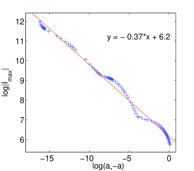
Figure 1: A logarithm of the maximal Riemann invariant (13) as a function of the distance from the critical amplitude, $a_{*}-a$, in the simulations with $\sigma_{r}=0.9,~{}\sigma_{z}=1.3$, and the fixed resolution $h=1/300$. The critical amplitude in this case is $a_{*}=7.3079082$, and the maximal curvature is $|I_{max}|\sim 10^{5}$ in the units of the total mass. The linear fit to the data (solid line) has the slope $\beta\simeq-0.37$. Notice the (quasi-) periodic “wiggle” of the data points about the straight line, which we interpret to signal periodic self-similarity of the critical solution.

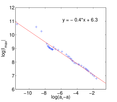
Figure 2: A plot similar to Fig. 1, but obtained with different parameters: $\sigma_{r}=\sigma_{z}=1$ and the resolution $h=1/300$. In this case the critical amplitude is $a_{*}=6.20021$. Remarkably, the slopes of the linear fits in both figures agree to within $8\%$.

The scaling can be envisaged by plotting the maximal value of the Riemann curvature invariant (13) as a function of the parametric distance from the critical amplitude, $a_{*}-a$; this is shown in Fig. 1. Each point here represents the global maximum $|I_{max}|$ computed during evolutions defined by $\sigma_{r}=0.9$ and $\sigma_{z}=1.3$, and the numerical parameters: $h=1/300,h_{t}/h=0.04,\mu_{1}=0.3,\mu_{2}=0.9,\kappa=1.7,\epsilon=0.6$. The solid line represents the least-squares linear fit to the data. The slope of the line, $\beta\simeq-0.37$, is in agreement with the exponent of the black-holes’ mass scaling, found in supercritical collapse by Abrahams and Evans [3]. The data depicted in Fig. 2 were obtained with a differently shaped initial wave, $\sigma_{r}=\sigma_{z}=1$, and the parameters $h=1/300,h_{t}/h=0.05,\mu_{1}=0.12,\mu_{2}=1.17,\kappa=1.7,\epsilon=0.8$. The threshold amplitude in this case is found with somewhat lesser accuracy, $a_{*}=6.20021\pm 0.00001$. However, the data is still fitted well with a straight line whose slope, $\beta\simeq-0.4$, coincides with the exponent in Fig. 1 to within $8\%$.

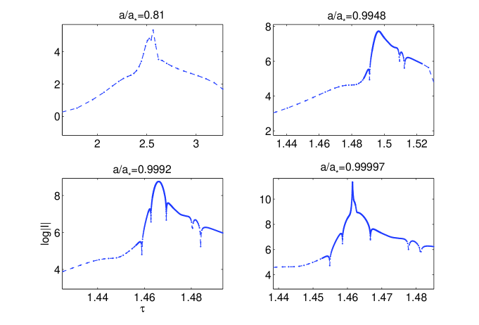
Figure 3: The dynamics of the logarithm of the Riemann invariant, $I$, as a function of the proper time $\tau(r_{*})$ for several values of $a/a_{*}$, obtained in the evolution of initial data defined by $\sigma_{r}=0.9,\sigma_{z}=1.3$, and the fixed resolution $h=1/300$. The variation of $I$ toward the accumulation, $\tau_{*}$, and away from it is accompanied by oscillations, whose number grows in the limit $a\rightarrow a_{*}$. The double dip in top right panel at about $\tau\simeq 1.51$ and in bottom panels near $\tau\simeq 1.48$ is a result of the interference between the main and a secondary reflection off the axis.

It is remarkable that despite the evolutions of the initial waves shown in Figs. 1 and 2 are dramatically different, the maximal curvatures in both cases follow a power-law with similar exponents. We verify that the same scaling again appears in simulations with other shape parameters and in all cases that resulting exponent is consistently in the range $\beta\simeq 0.37-0.4$. In addition, the scaling exponent within these bounds when we use coordinate conditions with different choices of $\mu$’s in (5) (see e.g. Figs. 1 and 2). While this does not test the rigidity of $\beta$ with respect to all possible coordinate conditions, this demonstrates relative consistency of the exponent within the large family of the gauges (5). We conclude that in the critical limit the maximal curvature predominantly scales as $|I_{max}|\propto(a_{*}-a)^{-\beta}$, with $\beta=0.385\pm 0.015$, where the errorbars represent the deviation from the average value computed over all initial data sets that we have evolved.

The distribution of data points in Figs. 1 and 2 has a striking property, namely the data “wiggle” about the linear fit. We note that similar wiggle was also observed in near critical collapse of scalar field. In that case it was attributed [22] to the periodic self-similarity found in that system, where the critical solution, $Z_{*}$, repeats on itself after a discrete period $\Delta$: $Z_{*}(\tau,r)=Z_{*}(\tau\,e^{\Delta},r\,e^{\Delta})$. Besides, [22] found that the period of the wiggle is $\Delta/(2\,\beta)$, and thus may, in principle, allow calculating the self-similarity scale $\Delta$ by measuring the slope and the period of the wiggle in a plot like ours Figs. 1 and 2. We believe that the quasi-periodic fluctuations of the points about the linear fit in these figures do signal discrete self-similarity, however our current data are insufficiently accurate and have too short a span to provide more quantitative estimate of the wiggle period, beyond a very rough value of anything between two and four.

Independent, and more direct signatures of discrete self-similarity are obtained by examining the behaviour of the curvature when $a\rightarrow a_{*}$. It turns out that in this limit, in addition to that $I$ attains increasingly larger maxima, the temporal variation of $I$ is also accompanied by increasing amount of oscillations. This is illustrated in Fig. 3, which shows the variation of $I$ as a function of the proper time, calculated at the accumulation loci, for a sequence of $a$’s. Figure shows that the amount of fluctuations—indicated by the peaks or inflection points—grows from one to three in the limit $a/a_{*}\rightarrow 1$ on both sides of the accumulation locus. Such an oscillatory behaviour is again reminiscent of the “echoing” in critical spherical collapse of scalar field (see e.g. Fig. 5 in [8] and Fig. 7 in [21]) and we interpret it as evidence of periodic self-similarity in our system as well.

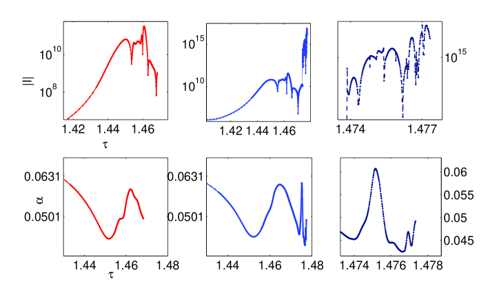
Figure 4: The echoing pattern obtained in the evolution of the initial data sets with $\sigma_{r}=0.9,~{}\sigma_{z}=1.3$ and $a=6.940$. Left panels show the low resolution runs that use 2 levels of AMR, with the base $h=1/128$, other panels were obtained using 4 AMR levels with the same base; the rightmost panels is the zooming of the late time behavior shown in middle panels. While the lower resolution runs diverge around $\tau\simeq 1.47$, the higher resolution runs extend beyond that, allowing to calculate additional echos. Notice that $I$ has sharper and easier to identify features than $\alpha$.

Like the power-law scaling of the maximal curvature, the echoing of our solutions in the near critical limit is independent of specific gauges or particular initial data sets. This is demonstrated in Fig. 4, which depicts temporal evolutions of the Riemann invariant and the lapse function found in simulations of the initial data characterized by $\sigma_{r}=0.9,~{}\sigma_{z}=1.3$, the gauge constants $\mu_{1}=0.3,~{}\mu_{2}=0.9$, and the amplitude $a=6.940$. The functions in left panels were computed using 2 levels of AMR, and the other panels were generated using 4 levels of AMR; in both cases the base-level resolution is $h=1/128$. Figure shows that the dynamics in this case involves more scatterings and interferences of the initial and secondary waves than e.g. in $\sigma_{r}=\sigma_{z}$ runs, depicted in Fig. 3.

In most cases higher resolution simulations run longer and allow computing more oscillations. Notice that the shapes of the curves in left and middle panels in Fig. 4 are essentially identical until $\tau\sim 1.47$. However, while the lower resolution runs diverge around that time due to formation of a singularity, the higher resolution evolutions continue beyond that, and develop additional echos that accumulate near $\tau_{*}\simeq 1.477M_{*}$, just before the numerics fails. The critical amplitude, determined in the 4-level AMR simulations is $a_{*}=6.9401$, and the accumulation loci occur are the origin. While we were unable to stabilize the 4-level evolutions for amplitudes beyond about $a\simeq 7$, in lower-resolution, 2-level runs we find a different critical solution with the amplitude, $a_{*}=7.246067$, where the accumulation locus lies at $\rho_{*}\simeq 0.23$, see Table 1. The total masses of the near critical spacetimes, the accumulation loci and such details of evolutions as the amount of secondary scatterings and interference’s, reflected in the strong variability of the curvature profile, and the total amount of gravitational radiation are different in near-critical evolutions in the 2 and 4-level AMR simulations. Nevertheless, the scaling and echoing constants appear to be nearly identical.

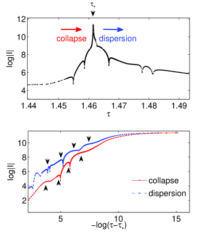
Figure 5: The typical temporal variation of the curvature invariant $I$ near the accumulation locus is oscillatory in time. Shown is the evolution of the initial data with $\sigma_{r}=\sigma_{z}=1$ and $a/a*=0.999998$. On each oscillation $\log|I|$ varies by $\Delta_{r}\simeq 1.1\pm 0.1$, which is close to the time period $\Delta_{\tau}\simeq 0.95\pm 0.15$ of the four oscillations around $\tau_{*}$.

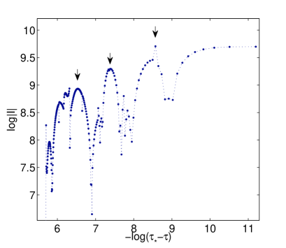
Figure 6: The variation of $I$ obtained in a 4-level AMR simulations initialized by $\sigma_{r}=0.9,~{}\sigma_{z}=1.3$, and $a/a*\simeq 0.99997$. The variation of $\log|I|$ on each oscillation (marked by arrows) is nearly equal to the temporal period of the echos, $\Delta_{r}\simeq\Delta_{\tau}\simeq 1.1$.

In order to estimate the period of the echos we plot in Fig. 5 the temporal variation of $I$ computed in the evolution of the initial data set having $\sigma_{r}=\sigma_{z}=1$ and $a=6.2002$. By measuring the distances between the peaks or inflection points—marked by arrows in Fig. 5—we find that the curvature fluctuates in time with the logarithmic period $\Delta_{\tau}=0.95\pm 0.15$ and that on each echo the logarithm of $I$ varies by approximately $\Delta_{r}\simeq 1.1\pm 0.1$. The errorbars here represent the maximal deviation from the average values of $\Delta_{\tau}$ and $\Delta_{r}$, measured in this figure. We note that both periods agree within the error-bars. A similar Fig. 6 shows the dynamics of $I$ against $\tau_{*}-\tau$, that was obtained in simulations with 4 levels of AMR, $\sigma_{r}=0.9,~{}\sigma_{z}=1.3$, and $a=6.940$, shown in right panels in Fig. 4. Although the resulting dynamics is quite complicated, featuring multiple scatterings and interferences, there are 3 prominent peaks—marked by the arrows in Fig. 6—that can be identified as echos. Their temporal period is $\Delta_{\tau}=1.10\pm 0.04$, and on each echo the logarithm of $|I|$ grows by a comparable amount $\Delta_{r}=1.12\pm 0.06$. We note that these values match within the errorbars, and are in a good agreement with the periods computed in Fig. 5.

The echoing is not specific to the curvature invariant $I$, other metric functions oscillate as well. However, while the echoes of $I$ are signalled by the sharp peaks the fluctuations of metric components are typically milder, showing up as inflection points (see bottom panels in Fig. 4). This makes $I$ a superior quantity for the purpose of measuring the echoing periods. Although we mainly discussed variations of $I$ at the location of its global maximum, we verified that curvature develops echoes in other locations as well, where, however, the amount of the echos and their amplitude is generally smaller than around the accumulation locus. Since away from the accumulation locus the curvature remains bounded in the critical limit we expect only a finite number of such oscillations.

We conclude this section by briefly discussing the accuracy of our code. While it was not possible to perform a direct convergence test of e.g. the critical amplitude or the scaling exponent, since changes of the resolution usually required readjustments of the dissipation, $\epsilon_{KO}$, and the constraint damping, $\kappa$ and the gauge parameters $\mu_{1},\mu_{2}$, which alter the “conditions of the convergence study”, that require all parameters except $h$ to stay fixed. Nevertheless, as indicated in Table 1 the critical amplitude seems to converge as a function of the resolution, at least in the equal-$\sigma$’s case. In addition, formal numerical convergence tests in individual, fixed amplitude simulations along with the demonstration that the Hamiltonian and the momentum constraints are satisfied during the evolutions were carried out in [5], indicating nearly second order convergence, and exponential decay of the $l_{2}$-norms of the constraints at late times.

The consistency of the scaling exponents obtained in simulations with a whole different set of parameters (see e.g. Figs. 1 and 2) indicates robustness of $\beta$, however the overall accuracy of our code can be estimated by changing only the numerical parameters. To this end we performed simulations with different damping and the Kreiss-Oliger dissipation constants $\kappa$ and $\epsilon_{KO}$, and otherwise similar parameters. Fig. 7 shows that $\beta$’s computed in two sets of simulations defined by $\kappa=1.4,\epsilon_{KO}=0.75$, and $\kappa=1.5,\epsilon_{KO}=0.85$ differ by less than $3\%$.

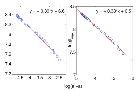
Figure 7: The logarithm of $|I_{max}|$ obtained in simulations with two distinct sets of the damping and dissipation constants: $\kappa=1.4,\epsilon_{KO}=0.75$ (right panel), and $\kappa=1.5,\epsilon_{KO}=0.85$ (left panel). We use same resolution of $h=1/300$, and all other equal parameters. The difference in $\beta$’s in this case is less than $3\%$, indicating the quality of our numerics.

4 Discussion

The ring-shaped accumulation loci that we observe in most evolutions of the time-symmetric Brill-wave initial data indicate that the critical solutions in these cases are genuinely different from those found by Abrahams & Evans [3] for the ingoing $l=2$ quasi-linear wave data, where the maximal curvature occurs at the origin. The black hole radii and their masses found in slightly super-critical evolutions in [3] are tend to zero in the critical limit, signalling so-called type II critical phenomenon, characterized by smooth transition between dispersion and black hole formation, see Ref. [2]. In our case, however, the radii of the accumulation loci are finite, as are the apparent horizons that form in supercritical collapse, engulfing the accumulation loci. Although, at present, neither our numerics is capable of finding apparent horizons very close to the threshold, $a_{*}\raisebox{-2.15277pt}{$\>\stackrel{{\scriptstyle\textstyle<}}{{\sim}}\>$}a\raisebox{-2.15277pt}{$\>\stackrel{{\scriptstyle\textstyle<}}{{\sim}}\>$}1.2\,a_{*}$, nor it allows to trace the evolution of the horizons to their endstate, it indicates that our critical solutions include quasi-stationary ring-shaped formations of finite size and mass.

The situation with the four and two levels AMR simulations is somewhat puzzling. While the two level simulations are clearly divergent near $a=6.9401$, which is determined as the critical amplitude in the four level runs, comparable in resolution unigrid runs do not encounter any particular difficulties at this amplitude. We believe such a behaviour may signal another, different critical solution, which is not resolved by the lower-dimensional unigrid simulations, and which destabilizes the less accurate two-level runs. However, whether this is indeed the case requires further investigation.

In all cases, we found strong evidence that in subcritical non-rotating axisymmetric vacuum collapse curvature exhibits a power-law scaling as a function of parametric distance from the threshold for black hole formation. We numerically evolved several sets of initial Brill-waves defined by fixed $\sigma_{r}$ and $\sigma_{z}$, and by a tuneable amplitude, $a$, and checked that in the limit $a\rightarrow a_{*}$, $|I_{max}|\propto(a_{*}-a)^{-\beta}$ with roughly the same exponent as that computed in supercritical regime by Abrahams and Evans [3], see Figs. 1 and 2. This demonstrates that quantities with same length dimensions—such as the black hole mass in [3] and the inverse curvature invariant $I_{max}^{-1}$ here—scale identically. We verified that the exponent is relatively insensitive to coordinate conditions. Since we find that the scaling occurs around a ring-shaped accumulation locus, which is different from the point-like one of [3], there is no a priori reason to expect the exponents in both cases to match. However, the exponents agree, and this, apparently, indicates that $\beta\simeq 0.35-0.4$ is truly universal and independent of the initial data, regardless of what critical solution these data may lead to.

There is evidence that the near critical solutions are periodically self-similar. Specifically, we observe that in the limit $a\rightarrow a_{*}$ the curvature invariant $I$ undergoes increasingly large number of oscillations, whose period in the proper time is approximately equal to the rate of variation of the curvature on each echo $\Delta_{\tau}\simeq\Delta_{r}\simeq 1.1$, see Figs. 3, 5 and 6. We note that the echoing periods reported in [3], $\Delta\sim 0.6$, differ from ours, which are roughly twice larger in magnitude. However, this is probably not too surprising since our critical solutions are different from theirs, and besides the period of any specific quantity will typically depend on the particular combinations of the metric and derivatives, comprising it (for instance, the quantity ${\partial}^{2}\Psi/{\partial}\tau^{2}$ is twice more variable than $\Psi$). An independent, if circumstantial, signature of discrete self-similarity is the distinctive “wiggle” of the data points about the leading power-law scaling of $|I_{max}|$, see Figs. 1 and 2, since exactly this kind of behavior is expected in the periodically self-similar systems [22].

An obvious limitation of the current simulations is their maximal resolution. Even though a relatively moderate numerical resolutions of $h\simeq 1/250-1/1000$ have already provided fruitful insights into the critical behavior, higher resolutions are needed in order to compute the scaling and echoing constants more accurately. We expect that much closer approach to threshold will be required. This should create a longer span of data, enabling a greater accuracy of linear fits in the plots like Fig. 1 and 2, which, in turn, will allow unambiguous computation of $\beta$ and of the wiggle period. A closer approach $a\rightarrow a_{*}$ should also multiply the number of the echoes, allowing a better estimate on their periods. Clearly, using numerical meshes of fixed size is not practical for probing the limit $a\rightarrow a_{*}$, rather AMR approach should be used. While we have already experimented with that, our runs often develop premature instabilities since in the near critical limit the system tends to be extremely sensitive to numerical and gauge parameters; for instance, in the 4-level simulations a slight variation of $\kappa$ by a mere $1\%$ ruins convergence. We are currently improving our code in order to locate the optimal parameter settings, which will enable us to edge the critical limit, the results of that study will be reported elsewhere.

References

References

- [1] M. W. Choptuik, “Universality And Scaling In Gravitational Collapse Of A Massless Scalar Field,” Phys. Rev. Lett. 70, 9 (1993).
- [2] C. Gundlach and J. M. Martin-Garcia, “Critical phenomena in gravitational collapse,” Living Rev. Rel. 10, 5 (2007)
- [3] A. M. Abrahams and C. R. Evans, “Critical behavior and scaling in vacuum axisymmetric gravitational collapse,” Phys. Rev. Lett. 70, 2980 (1993), A. M. Abrahams and C. R. Evans, “Universality in axisymmetric vacuum collapse,” Phys. Rev. D 49, 3998 (1994).
- [4] M. Alcubierre, G. Allen, B. Bruegmann, G. Lanfermann, E. Seidel, W. M. Suen and M. Tobias, Phys. Rev. D 61, 041501 (2000) [arXiv:gr-qc/9904013].
- [5] E. Sorkin, “An axisymmetric generalized harmonic evolution code,” Phys. Rev. D 81, 084062 (2010) [arXiv:0911.2011 [gr-qc]].
- [6] T. Koike, T. Hara and S. Adachi, “Critical behavior in gravitational collapse of radiation fluid: A Renormalization group (linear perturbation) analysis,” Phys. Rev. Lett. 74, 5170 (1995)
- [7] D. Garfinkle and G. C. Duncan, “Scaling of curvature in sub-critical gravitational collapse,” Phys. Rev. D 58, 064024 (1998)
- [8] E. Sorkin and Y. Oren, “On Choptuik’s scaling in higher dimensions,” Phys. Rev. D 71, 124005 (2005) [arXiv:hep-th/0502034].
- [9] H. Friedrich, “Hyperbolic Reductions For Einstein’s Equations,” Class. Quant. Grav. 13, 1451 (1996).
- [10] D. Garfinkle, “Harmonic coordinate method for simulating generic singularities,” Phys. Rev. D 65, 044029 (2002)
- [11] F. Pretorius, “Numerical Relativity Using a Generalized Harmonic Decomposition,” Class. Quant. Grav. 22, 425 (2005)
- [12] L. Lindblom and B. Szilagyi, “An Improved Gauge Driver for the GH Einstein System,” Phys. Rev. D 80, 084019 (2009) M. W. Choptuik and F. Pretorius, “Ultra Relativistic Particle Collisions,” Phys. Rev. Lett. 104, 111101 (2010)
- [13] D. R. Brill, “On the positive definite mass of the Bondi-Weber-Wheeler time-symmetric gravitational waves,” Annals Phys. 7, 466 (1959).
- [14] L. Lindblom, M. A. Scheel, L. E. Kidder, R. Owen and O. Rinne, “A New Generalized Harmonic Evolution System,” Class. Quant. Grav. 23, S447 (2006)
- [15] C. Gundlach, J. M. Martin-Garcia, G. Calabrese and I. Hinder, “Constraint damping in the Z4 formulation and harmonic gauge,” Class. Quant. Grav. 22, 3767 (2005) [arXiv:gr-qc/0504114].
- [16] F. Pretorius, “Simulation of binary black hole spacetimes with a harmonic evolution scheme,” Class. Quant. Grav. 23, S529 (2006) [arXiv:gr-qc/0602115].
- [17] E. Sorkin and M. W. Choptuik, “Generalized harmonic formulation in spherical symmetry,” Gen. Rel. Grav. 42, 1239 (2010) [arXiv:0908.2500 [gr-qc]].
- [18] A. M. Abrahams, K. R. Heiderich, S. L. Shapiro and S. A. Teukolsky, “Vacuum Initial Data, Singularities, And Cosmic Censorship,” Phys. Rev. D 46, 2452 (1992).
- [19] D. Garfinkle and G. C. Duncan, “Numerical evolution of Brill waves,” Phys. Rev. D 63, 044011 (2001) [arXiv:gr-qc/0006073].
- [20] Parallel Adaptive Mesh Refinement (PAMR) and Adaptive Mesh Refinement Driver (AMRD), http://laplace.phas.ubc.ca/Group/Software.html.
- [21] R. S. Hamade and J. M. Stewart, “The Spherically symmetric collapse of a massless scalar field,” Class. Quant. Grav. 13, 497 (1996) [arXiv:gr-qc/9506044].
- [22] C. Gundlach, “Understanding critical collapse of a scalar field,” Phys. Rev. D 55, 695 (1997) S. Hod and T. Piran, “Fine-structure of Choptuik’s mass-scaling relation,” Phys. Rev. D 55, 440 (1997)